Accelerating a Geometrical Approximated PCA Algorithm Using AVX2 and CUDA


1
Department of Electronics and Computers, Transilvania University of Brasov, 500036 Brasov, Romania
2
Quantum & Computer Engineering Department, Computer Engineering Research Group, Delft University of Technology, Mekelweg 4, 2628 CD Delft, The Netherlands
*
Author to whom correspondence should be addressed.
Remote Sens. 2020, 12(12), 1918; https://doi.org/10.3390/rs12121918
Submission received: 18 May 2020
/
Revised: 9 June 2020
/
Accepted: 9 June 2020
/
Published: 13 June 2020
(This article belongs to the Special Issue GPU Computing for Geoscience and Remote Sensing)
Abstract
:Remote sensing data has known an explosive growth in the past decade. This has led to the need for efficient dimensionality reduction techniques, mathematical procedures that transform the high-dimensional data into a meaningful, reduced representation. Projection Pursuit (PP) based algorithms were shown to be efficient solutions for performing dimensionality reduction on large datasets by searching low-dimensional projections of the data where meaningful structures are exposed. However, PP faces computational difficulties in dealing with very large datasets—which are common in hyperspectral imaging, thus raising the challenge for implementing such algorithms using the latest High Performance Computing approaches. In this paper, a PP-based geometrical approximated Principal Component Analysis algorithm (gaPCA) for hyperspectral image analysis is implemented and assessed on multi-core Central Processing Units (CPUs), Graphics Processing Units (GPUs) and multi-core CPUs using Single Instruction, Multiple Data (SIMD) AVX2 (Advanced Vector eXtensions) intrinsics, which provide significant improvements in performance and energy usage over the single-core implementation. Thus, this paper presents a cross-platform and cross-language perspective, having several implementations of the gaPCA algorithm in Matlab, Python, C++ and GPU implementations based on NVIDIA Compute Unified Device Architecture (CUDA). The evaluation of the proposed solutions is performed with respect to the execution time and energy consumption. The experimental evaluation has shown not only the advantage of using CUDA programming in implementing the gaPCA algorithm on a GPU in terms of performance and energy consumption, but also significant benefits in implementing it on the multi-core CPU using AVX2 intrinsics.

1. Introduction
Today, enormous amounts of data are being generated on a daily basis from social networks, sensors and web sites [1]. In particular, one type of multidimensional data which is undergoing an explosive growth is the remote sensing data.
Remote sensing is generally defined as the field or practice of gathering information from distance about an object (usually the Earth’s surface by measuring the electromagnetic radiation) [2]. The recent technological advances in both sensors and computer technology have increased exponentially the volume of remote sensing data repositories. For example, the data collection rate of the NASA Jet Propulsion Laboratory’s Airborne Visible/Infrared Imaging Spectrometer (AVIRIS) is 4.5 MB/s, which means that it can obtain nearly 16 GB of data in one hour [3].
The availability of new space missions providing large amounts of data on a daily basis has raised important challenges for better processing techniques and the development of computationally efficient techniques for transforming the massive amount of remote sensing data into scientific understanding. However, because much of the data are highly redundant, it can be efficiently brought down to a much smaller number of variables without a significant loss of information. This can be achieved using the so-called Dimensionality Reduction (DR) techniques [4]. These are mathematical procedures that transform the high-dimensional data into a meaningful representation of reduced dimensionality [5]. DR techniques are also referred to as projection methods, and are the widely used exploratory tools for applications in remote sensing due to a set of benefits that are bringing for remote sensing data analysis [6]:
- Plotting and visualizing data and potential structures in the data in lower dimensions;
- Applying stochastic models;
- Solving the “curse of dimensionality”;
- Facilitating the prediction and classification of the new data sets (i.e., query data sets with unknown class labels).
Of the several existing DR techniques, Projection Pursuit (PP) [7] and its particular form of Principal Component Analysis (PCA) [8] are being credited as two of the most popular dimensionality reduction techniques with numerous applications in remote sensing. PP is a Projection Index (PI)-based dimensionality reduction technique that uses a PI as a criterion to find directions of interestingness of data to be processed and then represents the data in the data space specified by these new interesting directions [9]. Principal Component Analysis [8] can be considered a special case of PP in the sense that PCA uses data variance as a PI to produce eigenvectors.
Such DR (like PP or PCA) have the disadvantage of being extremely computationally demanding, in consequence, their implementation onto high-performance computer architectures becomes critical especially for applications under strict latency constraints. In this regard, the emergence of high performance computing devices such as multi-core processors, Field Programmable Gate Arrays (FPGAs) or Graphic Processing Units (GPUs) [10] exhibit the potential to bridge the gap towards onboard and real-time analysis of remote sensing data.
PCA is a time and computational expensive algorithm, with two computationally intensive steps: computing the covariance matrix, and computing the eigenvalue decomposition of the covariance matrix. As a result of its nature, most PCA algorithms work in multiple synchronous phases, and the intermediate data are exchanged at the end of each phase, introducing delays and increasing the total execution time of the PCA algorithm. This is one of the reasons that has motivated the appearance in the recent literature of various implementations for the PCA algorithms in single-core systems, multi-core systems, GPUs and even on FPGAs.
In this context, this paper describes the parallel implementation of a PP-based geometrical approximated Principal Component Analysis algorithm, namely the gaPCA method. For validation, we applied gaPCA to a satellite hyperspectral image for dimensionality reduction. This method has been implemented in C++, Matlab and Python for our multi-core CPU tests, and PyCUDA and CUDA targeting an NVIDIA GPU. A comparative time analysis has been performed and the results show that our parallel implementations provide consistent speedups.
The main contributions of this work are as follows:
- We introduce four implementations of the gaPCA algorithm: three targeting multi-core CPUs developed in Matlab, Python and C++ and a GPU-accelerated CUDA implementation;
- A comparative assessment of the execution times of the Matlab, Python and PyCUDA multi-core implementations. Our experiments showed that our multi-core PyCUDA implementation is up to 18.84× faster than its Matlab equivalent;
- A comparative assessment of the execution times of the C++ single-core, C++ multi-core, C++ single-core Advanced Vector eXtensions (AVX2) and C++ multi-core AVX2 implementations. The multi-core C++ AVX2 implementation proved to be up to 27.04× faster than the C++ single core one;
- Evaluation of the GPU accelerated CUDA implementation compared to the other implementations. Our experiments show that our CUDA Linux GPU implementation is the fastest, with speed ups up to 29.44× compared to the C++ single core baseline;
- Energy consumption analysis.
The rest of the paper is organized as follows: Section 2 highlights related work in the field of projection pursuit algorithms; Section 3 describes the experimental setup—hardware, software and the data sets used for testing; Section 4 introduces the gaPCA algorithm with its applications in land classification; Section 5 describes the parallel implementations of the gaPCA algorithm using multi-core CPUs, CUDA programming and AVX2 intrinsics; Section 6 presents and analyzes the results obtained for each experiment. Finally, Section 7 concludes the paper.
2. Background and Related Work
2.1. Projection Pursuit Algorithms
Projection Pursuit is a class of statistical non-parametric methods for data analysis proposed initially by Friedman and Tukey in 1974 [7], which involves searching for directions in the high-dimensional space onto which the data can be projected to reveal meaningful low-dimensional insight into the data structures. Consequently, in Projection Pursuit, the key aspect is optimizing a certain objective function referred to as the Projection Index. A PI is a function which associates a data projection to a real value measuring how important that projection is (usually meaning how far from normality is).
Given the fact that the importance of the projection is dependent on the goal to be achieved (e.g., exploratory data analysis, density estimation, regression, classification, de-correlating variables), various PIs can be defined for each application (clustering analysis and detection [11,12], classification [13,14,15,16,17], regression analysis [18,19] and density estimation [20], leading to different indices for different projections (among these indices one can find entropy [21], variance, robust scale estimator [22], skewness [23], L1-norm [24]). One of the most popular PI is the variance of the projected data, defined by the largest Principal Components (PCs) of the PCA.
Due to the fact that Projection Pursuit methods execution time increases exponentially with the dimensionality of data, these algorithms tend to be computationally intensive. This motivated researches to find alternative approaches for pursuing interesting projection not only in terms of data structures, but also in terms of computational resources [25,26]. For example, in [27] a simple version of the Projection Pursuit-based estimator is proposed which is easy to implement and fast to compute.
The Quality of Projected Clusters (QPC) [28] projection aims at finding linear transformations that create compact clusters of vectors, each with vectors from a single class, separated from other clusters. Fast approximate version of QPC [29] proposes some modifications of the QPC method that decrease computational cost and obtains results of similar quality with significant less effort.
The study in [17] presents an accelerating genetic algorithm for the Projection Pursuit model based on genetic algorithm, which can effectively avoid the huge calculated quantity and slow speed of traditional genetic algorithm. The authors in [30] proposed a PI based on white noise matrix, which proved to reveal interesting features in high dimensions with low computational effort on both simulated and real data sets.
In [31], the algorithms are targeted to speeding up the covariance matrix computation rather than finding the eigenvalues of matrix (by showing that the covariance between two feature components can be expressed as a function of the relative displacement between those components in patch space) and it achieved around 10× speedups than the baseline implementation.
2.2. Parallel Implementations of PP Algorithms
In addition to algorithmic optimizations like the ones in the references mentioned above, many efforts made by the scientific community in the past decade focused on developing parallel implementations of a particular case of Projection Pursuit method, which is PCA, in order to achieve increased performance fostered by parallel architectures such as multi-core CPUs or GPUs.
In [32], Funatsu et al. proposed a PCA algorithm based on the L1-norm that to be up to 3× faster on the Geforce GTX 280 GPU architecture comparing with classical CPU. The results were verified by applying the algorithm in the field of facial recognition. In [33], Josth et al. presented two implementations of the PCA algorithm, first using the Streaming SIMD Extensions (SSE) instructions set of the CPU, and secondly using the CUDA technique on GPU architectures for RGB and spectral images. The results show speed-ups of around 10× (compared with a multi-threaded C implementation) which allows using PCA on RGB and spectral images in real time.
Another approach of the iterative PCA algorithm implementation on GPU which is based on the standard Gram-Schmidt orthogonalization was made in [34] by Andrecut. The author presented the comparison of the GPU parallel optimized versions, based on CUBLAS (NVIDIA) with the implementation on CBLAS (GNU Scientific Library) on the CPU and showed approximately 12× speedup for GPU.
In [35], a modified version of the fast PCA algorithm implemented on the GPU architecture was presented along with the suitability of the algorithm for face recognition tasks. The results showed approximately 20× faster results comparing with two other implementations of the fast PCA algorithm (the CPU implementation and the CPU sequential version). In a similar way, in [36] a fast non-iterative PCA computation for spectral image analysis by utilizing a GPU is proposed.
The paper in [37] presents a study of the parallelization possibilities of an iterative PCA algorithm and its adaptation to a Massively Parallel Processor Array (MPPA) manycore architecture (The Kalray MPPA-256-N which is a single-chip manycore processor that assembles 256 cores running at 400 MHz, distributed across 16 clusters), and achieved an average speedup of 13× compared to the sequential version. In [38] the authors present a study of the adaptation of the previous mentioned PCA algorithm applied to Hyperspectral Imaging and implemented on the same aforementioned MPPA manycore architecture.
In addition, the work in [39] presents the implementation of the PCA algorithm onto two different high-performance devices (an NVIDIA GPU and a Kalray manycore, a single-chip manycore processor) in order to take full advantage of the inherent parallelism of these high-performance computing platforms, and hence, reducing the time that is required to process hyperspectral images.
Reconfigurable architectures, like FPGAs, are also used for accelerating PP-based and PCA-related algorithms. In [40] a FPGA-based implementation of the PCA algorithm is presented as a fast on-board processing solution for hyperspectral remotely sensed images, while in [41] a parallel Independent Component Analysis (ICA) algorithm was implemented on FPGA. Furthermore, in [42], the authors propose an FPGA implementation of the PCA algorithm using High Level Synthesis (HLS).
Last but not least, cloud computing is also leveraged for improving performance and decreasing runtime: in [43], the authors proposed a parallel and distributed implementation of the PCA algorithm on cloud computing architectures for hyperspectral data.
This paper addresses the computational difficulties of a Projection Pursuit method named geometrical approximated PCA (gaPCA), which is based on the idea of finding the projection defined by the maximum Euclidean distance between the points. The difficulties arise due to the fact that gaPCA involves computing a large number of distances and we address them by proposing several parallel implementations of the method. Among them, an SIMD based method and a GPU implementation are compared and the results showed significant speedup.
3. Experimental Setup
3.1. Hardware
The CPU used in our experiments was AMD Ryzen 5 3600 [44]. The main characteristics of this processor are listed in Table 1. We used the MSI B450 GAMING PLUS mainboard with AMD B450 Chipset.
The GPU used in our experiments was the EVGA NVIDIA GeForce GTX 1650 [45]. The GPU specifications are shown in Table 2.
For measuring we used the energy consumption, we used the PeakTech 1660 Digital Power Clamp Meter [46], which provides a large variety of measuring functions (such as measurements for alternating current, alternating voltage, true power, apparent power, reactive power, energy, the power factor, frequency and phase angle), and a PC interface for data acquisition via USB 2.0 Interface.
3.2. Software
The experiments described in this paper were conducted on the above-mentioned AMD Ryzen 5 3600 and NVIDIA GeForce GTX 1650 system, running the Ubuntu 18.04.3 LTS 64 bit Operating System with the following software tools:
- Matlab R2019b with Matlab Parallel Computing Toolbox
- Python 3.6.8
- NVIDIA CUDA toolkit release 10.1, V10.1.243
- PyCUDA version 2019.1.2
- gcc version 7.4.0
3.3. Datasets
The experiments have been carried out on two data sets: the Pavia University [47] hyperspectral image data set, gathered by the Rosis sensor, having a number of 103 spectral bands, 610 × 340 pixels and a geometric resolution of 1.3 m, and the Indian Pines data set [48], gathered by the AVIRIS sensor over the Indian Pines test site in North-western Indiana and consists of 145 × 145 pixels and 200 bands. RGB representation of both datasets is illustrated in Figure 1.
In our experiments the image dimensions taken as input are: M (the image width), N (the image height) and P (the number of bands), giving rise to a [M × N, P] matrix. The testcases used to benchmark our gaPCA implementations involved taking 4 different crops of each of the two datasets (100 × 100, 200 × 200, 300 × 300 and 610 × 340 for Pavia University, and 40 × 40, 80 × 80, 100 × 100 and 145 × 145 for Indian Pines). For all test cases we maintained the full spectral information, i.e., all the available number of bands were considered: 103 for Pavia University and 200 for Indian Pines. The number of Principal Components computed was varied between 1, 3 and 5 in order to analyze the scaling effects of computing more than one component.
4. The gaPCA Algorithm
4.1. Description of the gaPCA Algorithm
gaPCA is a novel method that defines its Principal Components as the set of linear projections described by the maximum range in the data (as opposed to the canonical version of the PCA in which the Principal Components are those linear projections that maximize the variance of the data) and are computed geometrically, as the vectors connected by the furthest points. Hence, gaPCA is focused on retaining more information by giving credit to the points located at the extremes of the distribution of the data, which are often ignored by the canonical PCA.
In the canonical PCA method, the Principal Components are given by the directions where the data varies the most and are obtained by computing the eigenvectors of the covariance matrix of the data. As a result that these eigenvectors are defined by the signal’s magnitude, they tend to neglect the information provided by the smaller objects which do not contribute much to the total signal’s variance.
Among the specific features of the gaPCA method are an enhanced ability to discriminate smaller signals or objects from the background of the scene and the potential to accelerate computation time by using the latest High Performance Computing architectures (the most intense computational task of gaPCA being distances computation, a task easily implemented on parallel architectures [49]). From the computational perspective, gaPCA subscribes to the family of Projection Pursuit methods (because of the nature of its algorithm). These methods are known to be computationally expensive (especially for very large datasets). Moreover, most of them involve statistical computations, discrete functions and sorting operations that are not easily parallelized [50,51]. From this point of view, gaPCA has a computational advantage of being parallelizable and thus yielding decreased execution times (an important advantage in the case of large hyperspectral datasets).
To carry out gaPCA in the manner of PP analysis, we first have to define an appropriate Projection Index and a direction onto which the projection is optimal. A PI is a measure of the desirability of a given projection [52]. In PCA, which can be viewed as a special case of PP, this index is the variance of the projection scores. In gaPCA, the PI is the Euclidean distance among data points. A high PI (given by large distance between data points) suggests important features, in terms of divergence from normality, which is a desired objective of Projection Pursuit techniques in general. In the field of hyperspectral imagery, if a PI attains a high value, it usually indicates a spectral characteristic different than that of the background, very important for object detection, identification of spectral anomalies, regardless of their relative size.
Given a sample of p-dimensional points, , in order to form a univariate linear projection of X, we define a as a p-dimensional normalized vector determined by the two p-dimensional points separated by the maximum Euclidean distance:
with
where denotes the Euclidean distance.
The gaPCA projection index function can be defined as:
Then, the projected data of X can be described as:
resulting in a new representation for each of the p dimensional points in a n-dimensional space.
To find a set of orthogonal projections, we have to reduce the rank of the data matrix by projecting it onto the subspace orthogonal to the previous projections. All the points in X are projected onto the hyperplane H, determined by the normal vector a and containing m (the midpoint of the segment that connects the two points):
This results in a set of projections of the original points, , computed using the following formula:
To further seek a linear projection onto the new dimensions, all the above steps are computed iterativelly, giving rise to a direction matrix A, so that the projection data can be rewritten as:
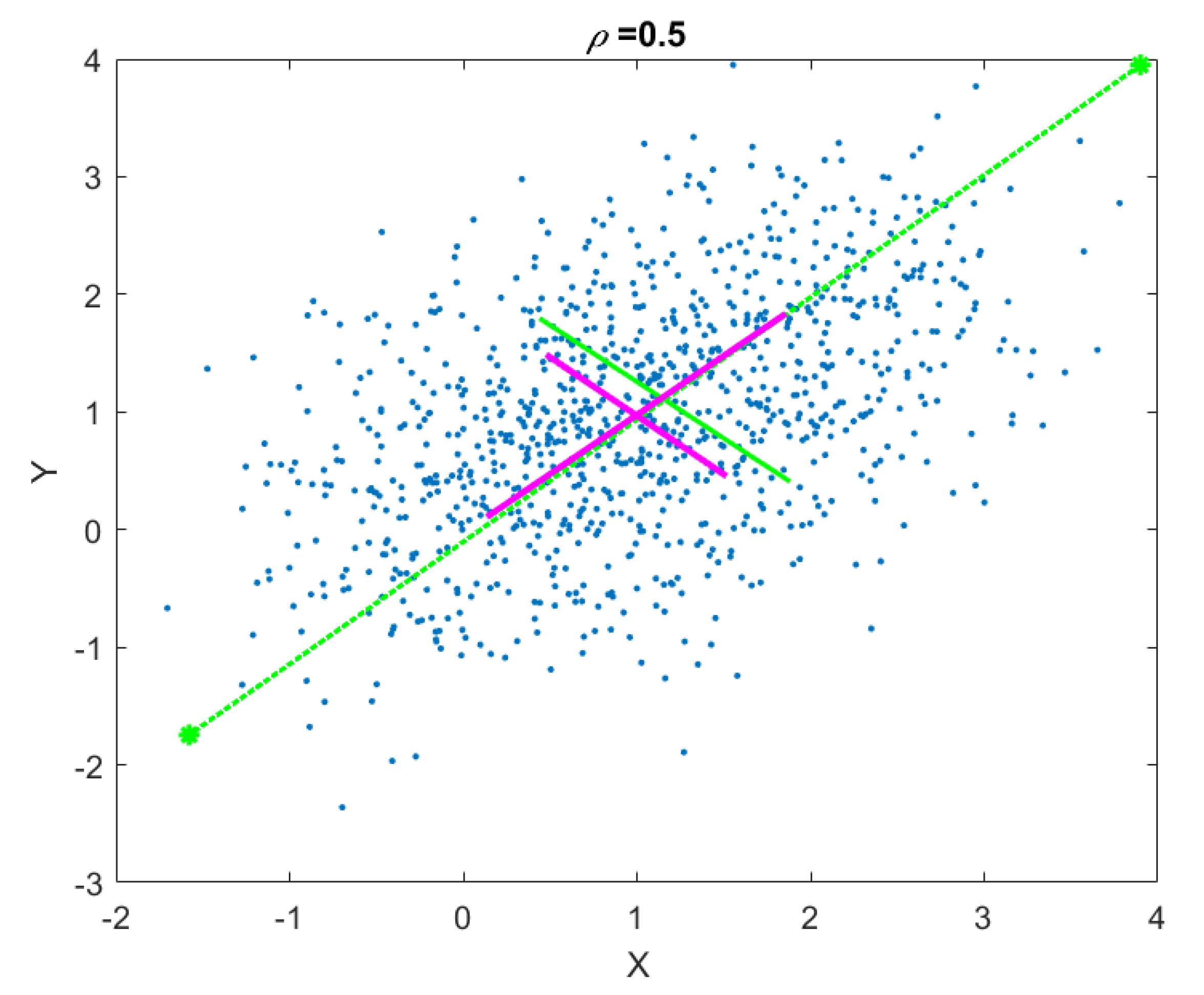
This sequence of operations can be repeated until the rank of the data matrix becomes zero. The end result is an orthogonal matrix, where each column is a projection vector. A graphical illustration of the computed gaPCA components vs. canonical PCA components is shown in Figure 2.
gaPCA is a geometric construction-based approach for PCA approximation, which was previously validated in applications such as remote sensing image visualization [53] and face recognition [54]. Moreover, gaPCA was shown [55] to yield better performance in land classification accuracy than the standard PCA, with the most remarkable results recorded in the cases of preponderantly spectral classes. In such classes the standard PCA’s performances are lower due to its loss in spectral information, that restrain its ability to discriminate between spectral similarities. Consequently, gaPCA is more suitable for hyperspectral images with small structures or objects that need to be detected or where preponderantly spectral classes or spectrally similar classes are present [55].
4.2. gaPCA in Land Classification Applications
To show the performance and efficiency of gaPCA as a Dimensionality Reduction algorithm in land classification applications, we have compared the gaPCA approach in the field of classification with the standard PCA algorithm as benchmark for the assessment of the gaPCA method.
Both methods were used on the Indian Pines and Pavia University datasets for dimensionality reduction, and for each data set the number of Principal Components computed was selected in order to achieve the best amount of variance explained (98–99%) with a minimum number of components (10 for the Indian Pines data, 4 for Pavia University).
The first Principal Components obtained after the implementation of each of the PCA methods represent the bands of the images on which the classification was performed (the input), using the ENVI [56] software application. Maximum Likelihood Algorithm (ML) and the Support Vector Machine Algorithm (SVM) were used for classifying both the standard PCA and the gaPCA image, for both datasets. The classification accuracy was assessed by generating a sub-set of randomly generated pixels, based on which a visual comparison with the groundtruth image of the test site at the acquisition moment was performed.
We assesed the classification accuracy of each method with two metrics: the Overall Accuracy (OA representing the number of correctly classified samples divided by the number of test samples) and the kappa coefficient of agreement (k, which is the percentage of agreement corrected by the amount of agreement that could be expected due to chance alone).
In order to assess the statistical significance of the classification results provided by the two methods, the McNemar’s test [57] was performed for each classifier (ML and SVM), based on the equation:
where represents the number of samples missclassified by method i, but not by method j. For , the overall accuracy differences are said to be statistically significant.
4.2.1. Indian Pines Dataset
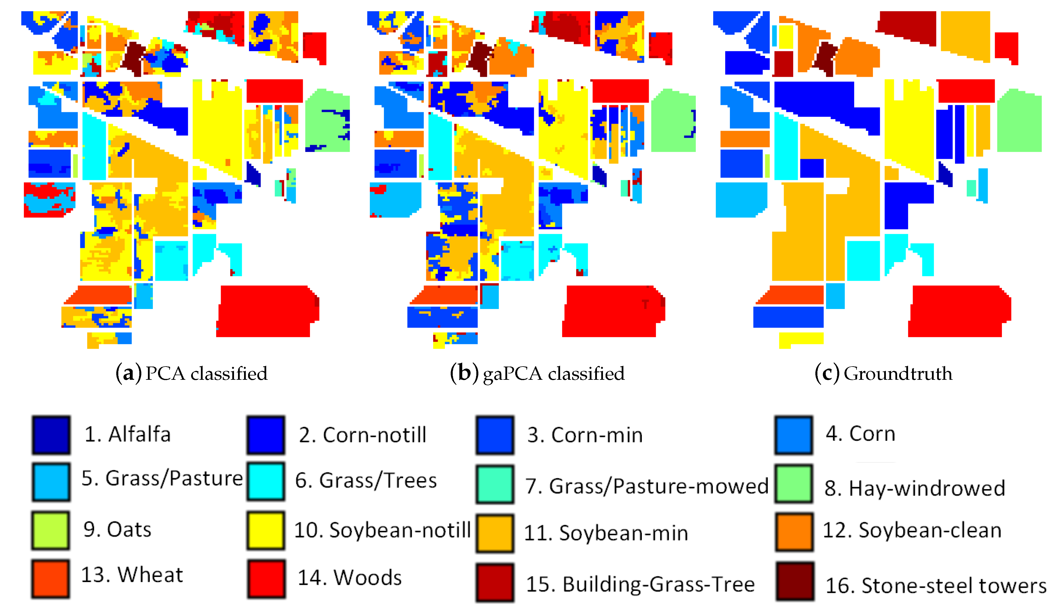
Performing land classification on the Indian Pines dataset is a challenging task due to the large number of classes on the scene and the moderate spatial resolution of 20 m and also due to the high spectral similarity between the classes, the main crops of the region (soybeans and corn) being in an early stage of their growth cycle. The classification results of the Standard PCA and the gaPCA methods are shown in Figure 3a,b along with the groundtruth of the scene at the time of the acquisition of the image (c). The Figure illustrates that although both classified images look noisy (because of the abundance of mixed pixels), the classification map obtained by the gaPCA is slightly better.
In Table 3 we summarized the classification accuracy of the two methods for each of the classes on the scene along with the Overall Accuracy of both methods with the ML and SVM algorithms. A set of 20,000 randomly generated pixels, uniformly distributed in the entire image were used for testing. The gaPCA OA is higher than the one scored by the standard PCA and the classification accuracy results for most classes are better. One reason for these results is that PCA makes the assumption that the features that present high variance are more likely to provide a good discrimination between classes, while those with low variance are redundant. This can sometimes be erroneous, like in the case of spectral similar classes. There is an important difference in the case of sets of similar class labels. gaPCA scored higher accuracy results for the similar sets of Corn, Corn notill, Corn mintill and also for Grass-pasture and Grass-pasture mowed than those achieved by the Standard PCA, demonstrating the ability of the method to better discriminate between similar spectral signatures.
4.2.2. Pavia University Dataset
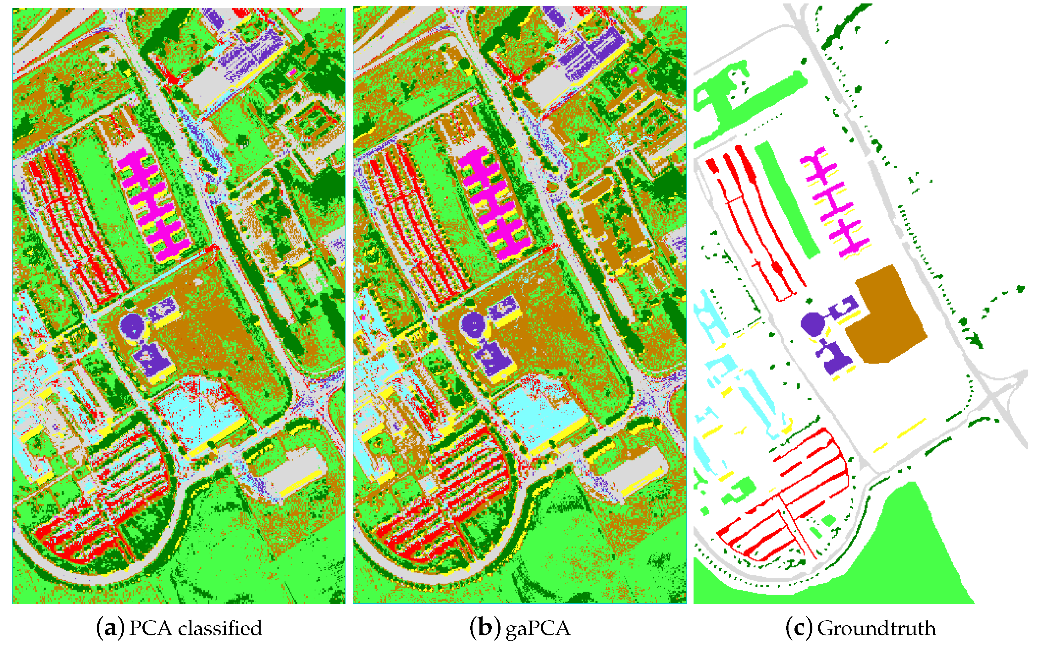
Figure 4 shows the images achieved with the Standard PCA method (a) and the gaPCA method (b) classified with the ML Algorithm and the groundtruth of the scene (c).
The classification results (for 1000 test pixels) using either ML or SVM are displayed in Table 4, showing the classification accuracy for each class and the OA. The results show gaPCA scored the best OA and classification accuracy for most classes.
The classification accuracies report better performances for gaPCA in interpreting classes with small structures and complex shapes (e.g., asphalt, bricks). This confirms the interest accorded by the gaPCA to smaller object and spectral classes leading to less false predictions compared to the standard PCA for this classes. This is more obvious for classes such as bricks where confusion matrix shows a misinterpretation with gravel and for asphalt confused with bitumen.
The reason behind these confusions is the spectral similarity between the two classes and not to the spatial proximity (Table 5), proving that gaPCA does a better job in discriminating between similar spectral classes because unlike PCA it is not focused on classes that dominate the signal variance.
In light of these results, gaPCA is confirmed to have a consistent ability when classifying smaller objects or spectral classes, proving the hypothesis that it has a superior ability in retaining information associated to smaller signals’ variance.
5. Parallelization of the gaPCA Algorithm
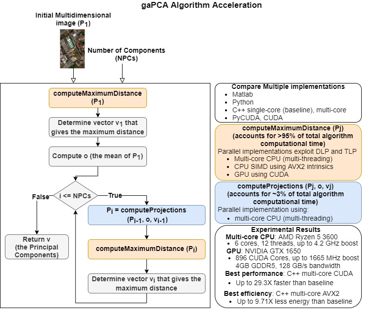
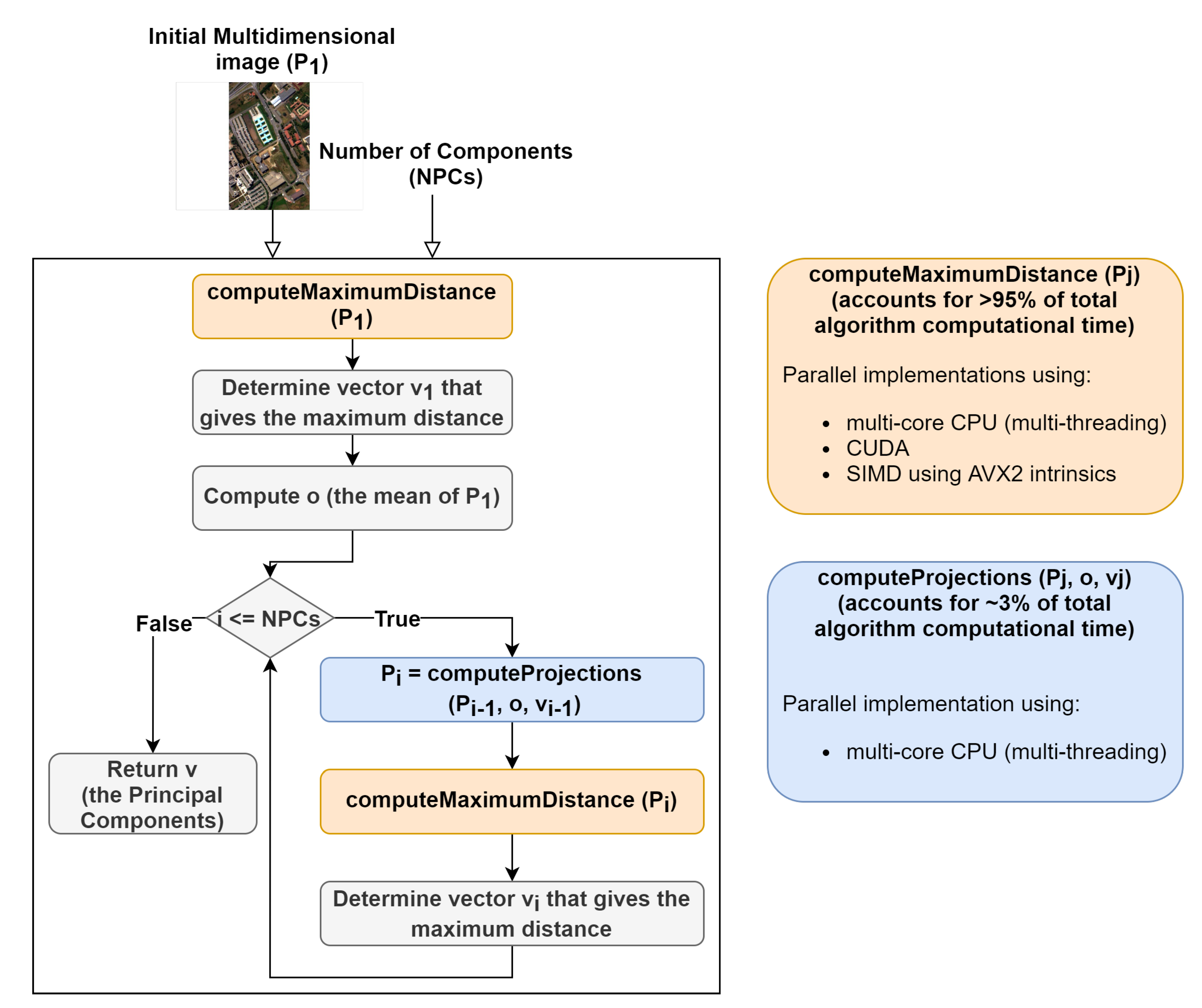
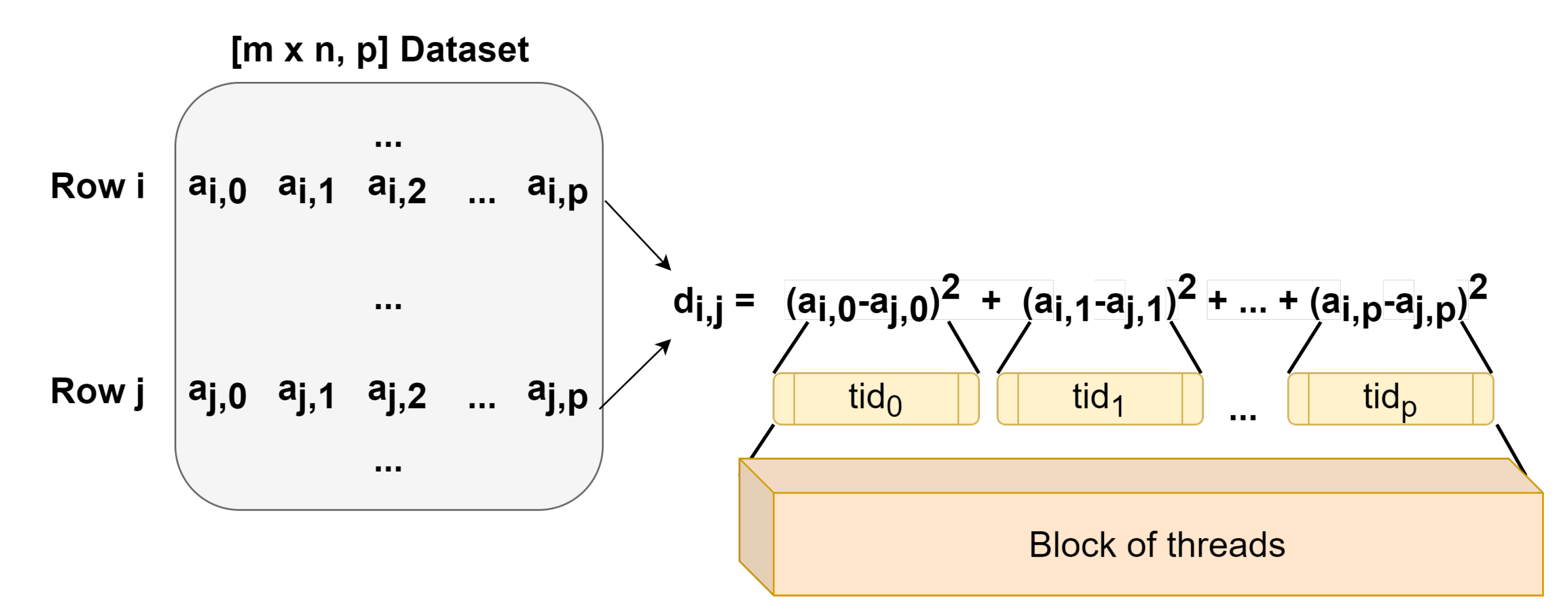
The first step was to perform a profiling of the code in order to assess what are the most time- and computation-consuming subroutines and which of them are appropriate for parallel implementations. A detailed perspective on the gaPCA algorithm and its sub-routines is shown in Figure 5. As expected, the code profiling analysis showed that by far the computation of the Euclidean distances between the pixels was the most time consuming task, accounting for approximately 95% of the total running time of the algorithm for any given dataset. The second most time consuming stage of the gaPCA algorithm is the projection of the data on the hyperplane orthogonal to each of the vectors computed, accounting for just 3% of the total computational time of gaPCA. Based on the time profiling results, we focused our efforts on parallel implementations for these two subroutines. Three implementations: CPU multi-threading, CUDA and SIMD AVX2 were ealborated for the Euclidean distance function (), which is by far the most time consuming and also it’s computational complexity (pariwise distance computations on a large dataset) fostered the use of the above-mentioned technologies. A diagram depicting the computation of one iteration of the Euclidean distances function is shown in Figure 6. For the subroutine responsible for computing the data projections on the hyperplane (), a CPU multi-core parallel implementation was elaborated.
Our research focused on two main aspects. First, on the efficient parallel implementation of the gaPCA algorithm using SIMD instruction set extensions, multi-threading and GPU acceleration. Second, on providing a comparison of the above mentioned implementations in terms of time and energy performance onto two different computing platforms: a PCI Express GPU accelerator from NVIDIA and a 64-bit x86 CPU from AMD.
The main idea behind parallelizing the gaPCA algorithm was to take advantages from both thread level parallelism and data level parallelism in order to gain higher performance. As a result that the gaPCA algorithm possess a massive data parallelism (with the sequence of operations computing the Euclidean distance between each pair of n-dimensional points executed for a large number of inputs), it is a good candidate for implementing CPU Data Level Parallelism (DLP) with SIMD.
5.1. Matlab, Python and PyCUDA Implementations
The initial implementation (Listing A1 in Appendix A) [49] was developed in Matlab using the specific instructions from the Matlab Parallel Computing Toolbox. The test runs were performed in Matlab R2019a, on the Linux Ubuntu 18.04 operating system. The instruction executes for-loop iterations in parallel on a parallel pool of workers on the multi-core computer or cluster. The default size of the pool of workers is given by the number of physical cores available.
The next two are Python implementations, targeting parallel execution on a multi-core CPU and a NVIDIA GPU, respectively. Both are based on the Python Numba and Numpy libraries; the CPU multi-core parallel execution was achieved using Numba JIT compiler, while the GPU CUDA version has been implemented using the PyCUDA Python library [58]. Python [59] is a high level programming language. It has efficient high-level data structures and a variety of dedicated libraries which recommends it both for scientific and real-time application. Numba [60] is an open source JIT compiler that translates a subset of Python and NumPy code into fast machine code. Numba can automatically execute array expressions on multiple CPU cores and makes it easy to write parallel loops.
Our second implementation (Listing A2 in Appendix A) was developed in Python using the Numba compiler. The test runs were performed in Python3, on the Linux Ubuntu 18.04 operating system. The decorator added before the definition of the Python function, specifies that Numba will be used. Numba’s CPU detection also enables LLVM [61] to autovectorize for appropriate SIMD instruction set: SSE, AVX, AVX2, AVX-512. The parallel option () enables a Numba transformation pass that attempts to automatically parallelize and perform other optimizations on the function. Furthermore, it offers support for explicit parallel loops. Consequently, Numba’s was used (instead of the standard ) to specify that the loop should be parallelized. A thread pool is automatically started and the tasks are distributed among these threads.Typically the pool size is equal to the number of cores available on the machine (6 in our case). However, this may be controlled through the variable. The is a function from the Python’s Numpy scientific package used to compute the norm of a vector or a matrix, in our case the Frobenius norm of the difference between the two vectors, equivalent to the Euclidean distance between the two).
CUDA Implementation
Our CUDA kernel was designed in order to have a block of threads compute one element of the distance matrix, with each thread computing the square distance between the corresponding elements of the two rows in the input matrix. In the example illustrated in Figure 7, the dataset a is the input matrix, whose rows contain the pixels’ values in every spectral band. The block of threads computes the distance between rows i and j, with each thread computing . After all threads in the block finish the tasks assigned (passing a synchronization phase), the squared values computed by the threads are added in a parallel tree reduction manner to obtain the total distances between the rows i and j of the input dataset a.
Listing A3 in Appendix A shows the pseudocode for the CUDA kernel (the Euclidean function). This function takes as input matrix X and returns C, a three element array containing the maximum distance () and the indexes of the corresponding two furthest points from matrix X ( and ).
In the CUDA kernel, we used a shared memory vector named , where each thread computes its corresponding squared difference. After all the threads in a block complete this step (ensured by calling the method), we perform parallel tree reduction as shown in the code excerpt from Listing A4, obtaining the final distance value. Finally, the thread with in each block compares the current computed distance with the previous existing maximum distance, and updates the maximum distance (and its corresponding indexes) if it is the case.
5.2. C++ Implementations
The first C++ implementation is a single-core one. For the second C++ multithreading implementation, we used OpenMP [62], a simple C/C++/Fortran compiler extension, which allows adding multithreading parallelism into existing source code.
In Listing A5 in Appendix A, the section of code that runs in parallel is marked accordingly by the pragma omp parallel compiler directive, that will cause the threads to form before the section is executed. This directive does not create a pool of threads, instead it take the team of threads that is active, and divide the tasks among them. The pragma omp for directive divides the distances computations between the pool of threads, which are run simultaneously. Each thread computes a distance between two rows of the matrix.
For the third C++ implementation, besides OpenMP, we have also employed SIMD instruction set extensions, for exploiting the avaliable DLP. SIMD instructions work on wide vector registers. Depending on the specific SIMD instruction set extension employed, the width of the vector registers ranges from 64 bits to 512 bits (e.g., MultiMedia eXtensions (MMX) [63], SSE [64], AVX [65]). In order to achieve 100% efficiency, the input array size should be a multiple of the width of the vector registers (e.g., 4, 8, 16 or 32 16-bit data elements); however, for large input array sizes, this does affect performance and high speedups can be achieved.
In our experiments, we employ the AMD Ryzen 5 3600 CPU [44] which supports the AVX2 [66] SIMD instruction set extension. An AVX2 vector register uses dedicated 256-bit registers, corresponding to the the float, double and int C/C++ types, and may store 8 double precision floating point numbers or 16 integer values, for example. After profiling the data, we choose to represent them as 16-bits integers, using type vectors, containing 16 integers represented on 16 bits. For storing and manipulating the data, we used the AVX2 intrinsic functions, available in the Intel library header . Intrinsics are small functions that are intended to be replaced with a single assembly instruction by the compiler.
One of the major challenges arising when vectorizing for SIMD architectures, is the handling of memory alignment. SIMD instructions are sensitive to memory alignment, and there are dedicated instructions for accessing unaligned and aligned data. As a result that each register size has a corresponding alignment requirement (i.e., the 256-bit Intel AVX registers have an alignment requirement of 32 bytes), attempting to perform an aligned load, or store, on a memory operand which does not satisfy this alignment requirement will generate errors [67]. There are several different methods for memory alignment. As shown in Listing A6 in Appendix A, we used the alignment macros defined in the header , providing the macro and the corresponding _ keyword, for alignment of a variable.
Listing A7 in Appendix A provides the code for computing the distances between two arrays, and , of length , using AVX2 intrinsics functions. To load the arrays of values into memory, we used the intrinsic . The was used to subtract each pair of 16-bit integers in the 256-bit chunks and the values obtained were then multiplied using the intrinsic. The second for loop of the function deals with the left-overs of the input arrays (in case that they are not multiple of 16, the sum of the differences between the remaining values is computed using standard C++ instructions). The sum of the squared differences was computed with another C++ function based on SIMD instructions, showed in Listing A8 in Appendix A.
6. Results and Discussion
To evaluate the gaPCA algorithm acceleration, we build a benchmark in which we measured the amount of time the algorithm took to execute on every testcase of the two datasets mentioned above, for 1, 3 and 5 Principal Components. For each of the above mentioned image sizes, we ran the algorithm with the specified number of computed Principal Components, several times for each test (in order to minimize the overhead time associated with the cache warming [68]) and averaged the result. The speedup was then computed as the division between the averaged time of each implementation (e.g., single/multi-core CPU, SIMD-augmented CPU, GPU) for the same image size and number of computed Principal Components.
6.1. Execution Time Performance
6.1.1. Matlab vs. Python and PyCUDA
The first comparative evaluation was performed between the execution times of the Matlab, Python and PyCUDA implementations of the gaPCA algorithm. The execution times were measured for all the above-mentioned image crops of the Indian Pines and the Pavia University dataset, for a number of 1, 3 and 5 computed Principal Component(s) (PCs), for 2 consecutive runs.
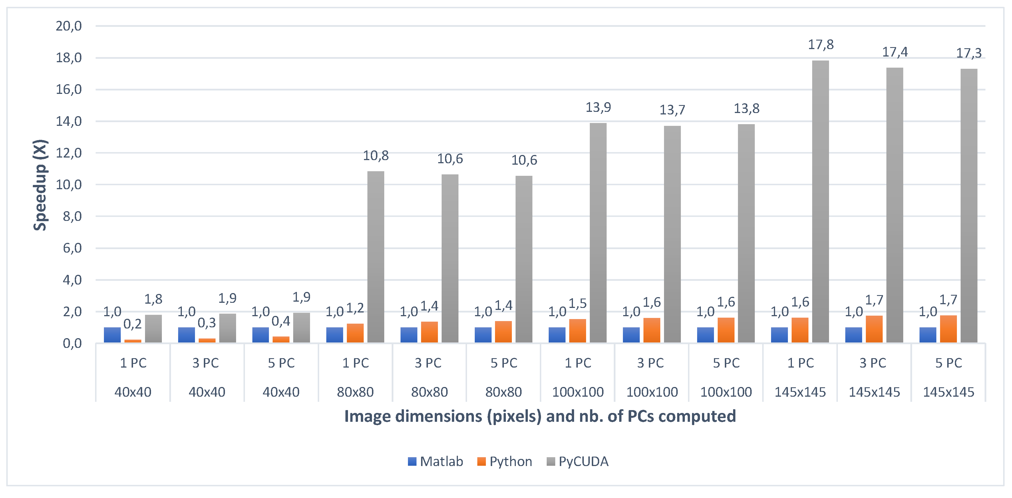
Table 6 shows the timing results for the three implementations, for each test case of the Indian Pines dataset. Similarly, Table 7 shows the timing results for the test cases of the Pavia University dataset. Figure 8 and Figure 9 present the speedup between the three implementations (with the Matlab implementation taken as a baseline for comparison) for all the test cases of the Indian Pines and the Pavia University, respectively.
For the first test case (Indian Pines), the Matlab implementation outperforms its Python equivalent, being with up to 4.58× for the 40 × 40 image crops, while for the other image sizes (80 × 80, 100 × 100 and 145 × 145) the Python implementation is faster. For the second test case (Pavia University), we can notice that the Matlab implementation is faster than the Python one with approximately 20% on average (ranging from 4% for the 200 × 200 and 5 PCs dataset to 42% for the 100 × 100 and 1 PC dataset).
One of the major factors influencing the differences in speedup between the Matlab implementation and its Python counterpart can be explained by the overheads associated with each environment’s compiler and the deployed components: a startup delay while the data is loaded or data marshaling associated with deploying certain libraries. Matlab employs a just in time compiler to translate code to machine binary executables. This substantially increases speed and is seamless from the user perspective since it is performed automatically in the background when a script is run. The python Numba Project has developed a similar just in time compiler, but the speedup is actually very small in case of using “non-native” python code (NumPy functions which cannot be compiled in optimal ways).
A second factor causing poor performance for Python as compared to Matlab for the smaller image crops, is the fact that in general, NumPy’s speed comes from calling underlying functions written in C/C++/Fortran. NumPy performs well when these functions are applied to whole arrays. In general, poorer performance is achieved when applying NumPy functions on smaller arrays or scalars in a Python loop (for the smaller dataset dimensions the Matlab speedup is higher than for the larger datasets). It is also notable that Matlab’s Parallel Toolbox is limited to 12 workers, whereas in Python there is no limit to the number of workers.
When comparing the two CPU multi-core implementations (Matlab and Python) with the GPU implementation (PyCUDA), the speedups show that the GPU implementation of the gaPCA algorithm is up to 17.82× faster (for Indian Pines) and up to 18.84× faster for the Pavia University dataset than the Matlab CPU implementation of the same algorithm taken as reference for comparison. One can notice that the greatest speedup is registered for the test cases with 1 computed principal component, due to the fact that for the smaller dataset sizes more of the data can fit into caches and the memory access time reduces dramatically, which causes the extra speedup in addition to that from the actual computation. In addition, the GPU speedup is slightly smaller for 3 and 5 computed Principal Components, due to the fact that unlike the CPU execution times which grow unlinear, the GPU execution time grows linear.
6.1.2. C++ Single Core vs. Multicore
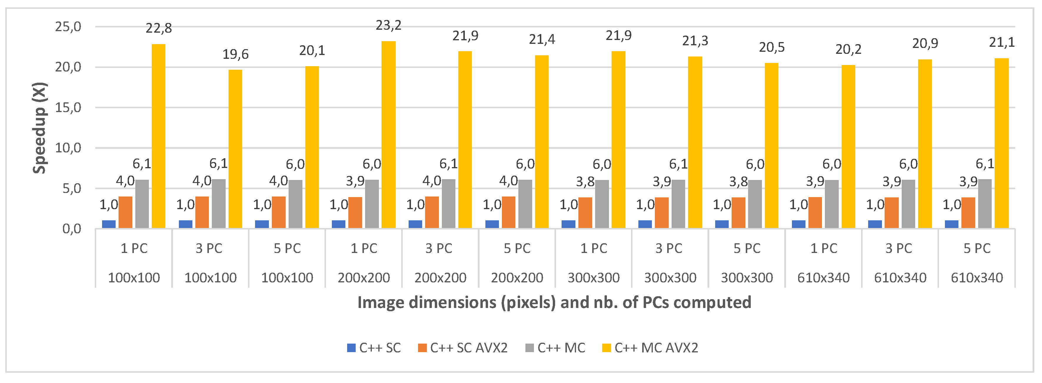
The second comparative evaluation was performed between the execution times of several C++ implementations: single core (C++ SC), single core with AVX2 intrinsics (C++ SC AVX2), multi-core (C++ MC) and multi-core using AVX2 intrinsics (C++ MC AVX2). The execution times were again measured for all image crops of the Indian Pines and the Pavia University dataset, for 1, 3 and 5 computed principal component(s) and averaged between 2 consecutive runs. Table 8 shows the timing results for the four implementations, for each test case of the Indian Pines dataset. Similarly, Table 9 shows the timing results for the test cases of the Pavia University dataset.
The speedups between the four implementations (with the single core implementation taken as a baseline for comparison) are shown in Figure 10 and Figure 11, for all the test cases of the Indian Pines and the Pavia University, respectively. The results show that the single-core AVX2 implementation is almost 4 times faster on average (3.90×) than the single core one for Pavia and 4.6 times faster on average for the Indian Pines testcases. The speed-up is slightly higher for Indian Pines due to the fact that this dataset has more spectral information (more bands, 200 vs. 103 as previously mentioned) which leads to more data being processed using AVX2 instructions thus increasing the efficiency and decreasing the execution time.
With regard to the multi-core implementation, the speed-up is consistent between the two datasets, and is on average 6 times faster than the single core version (6.04× for Pavia and 5.98× for Indian Pines). This is consistent with the number of cores (6) of the CPU on which the tests were carried. As expected, the multi-core AVX2 implementation yielded the best results with an average speed-up of 21.24× for Pavia and 23.92× for the Indian Pines testcases. The slightly better speed-up in the case of Indian Pines is again caused by the higher spectral dimension of this dataset, as explained above.
6.1.3. C++ Multi Core vs. CUDA
The final comparative evaluation was performed between the execution times of the three parallel C++ implementations: multi-core (C++ MC), multi-core using AVX2 intrinsics (C++ MC AVX2) and multi-core with CUDA programming (C++ MC CUDA). The execution times were again measured for all image crops of the Indian Pines and the Pavia University dataset, for 1, 3 and 5 computed principal component(s) and averaged between 2 consecutive runs. Table 10 shows the timing results for the three implementations, for each test case of the Indian Pines dataset. Similarly, Table 11 shows the timing results for the test cases of the Pavia University dataset.
The speedups between the three implementations (with the standard multi-core implementation taken as a baseline for comparison) are shown in Figure 12 and Figure 13, for all the test cases of the Indian Pines and the Pavia University, respectively. The results show that the multi-core AVX2 implementation is on average 3.52 times faster than the standard multi-core one for Pavia and 4 times faster on average for the Indian Pines testcases. This difference in speedup is caused by the same spectral dimensionality difference between the two datasets previously addressed.
With regard to the multi-core CUDA implementation, this was shown to be 4.85× faster on average than the standard multi-core version for Pavia and 4.14× faster on average for the Indian Pines testcases. It can be noticed that for the smaller crop sizes the speed-up is significantly lower or the CUDA version is even slower than the MC AVX2 implementation for the smallest crop size (e.g., for Indian Pines 40 × 40 and 1PC is 1.49× vs. 3.58× for MC AVX2). This is due to the CUDA computational overhead (i.e., copying the data from CPU memory to GPU memory and reverse). The impact of the overhead is reduced as the dataset size increases. This also explains the the speed-up difference between the two datasets which is reversed compared to the other comparisons discussed above, with a higher speed-up for Pavia and lower for Indian Pines. This is due to the fact that Indian Pines has a much smaller spatial resolution than Pavia (145 × 145 vs. 610 × 340) and for the smallest crop size (40 × 40) the CUDA computational overhead surpasses the acceleration gain.
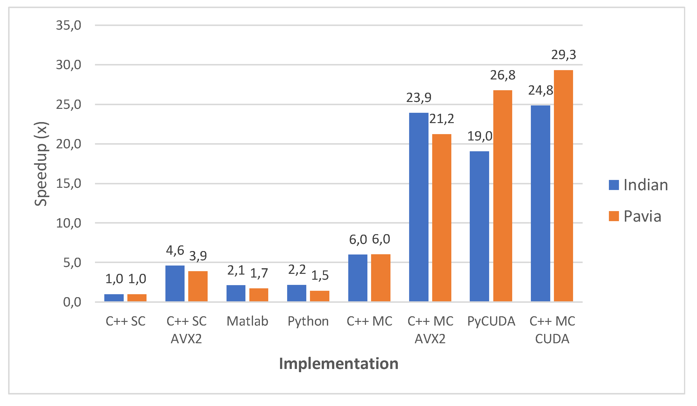
Figure 14 shows a comparison of all implementations in terms of speed-up compared to the C++ single-core version taken as baseline. This comparative perspective confirms that the two CUDA-based implementations (C++ MC CUDA and PyCUDA) yield the highest speed-ups, followed closely by the C++ MC AVX2 version. The C++ MC CUDA is faster than the PyCUDA version on average with 9.3% for Pavia and with aprrox. 30% for Indian Pines, which is explained by the fact that aside from the CUDA kernel, C++ multi-core code proved to be faster than its Python equivalent. Moreover, both show better speed-ups for Pavia than for Indian Pines, which is consistent since both share the same CUDA kernel.
The C++ MC AVX2 implementation shows a reversal of this trend - Indian Pines results having a slightly higher speed-up than Pavia—results which are consistent with the C++ SC AVX2 version where we notice the same trend. The probable cause is related to the spatial and spectral characteristics of the two datasets. Indian Pines has a lower spatial resolution but a higher spectral resolution than Pavia, and the spectral resolution impacts the number of AVX2 operations carried out. This leads to Indian Pines benefiting from AVX2 acceleration to a higher degree than Pavia.
6.2. Energy Efficiency
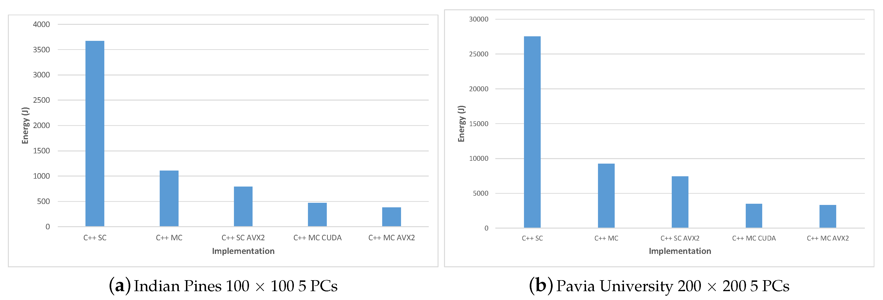
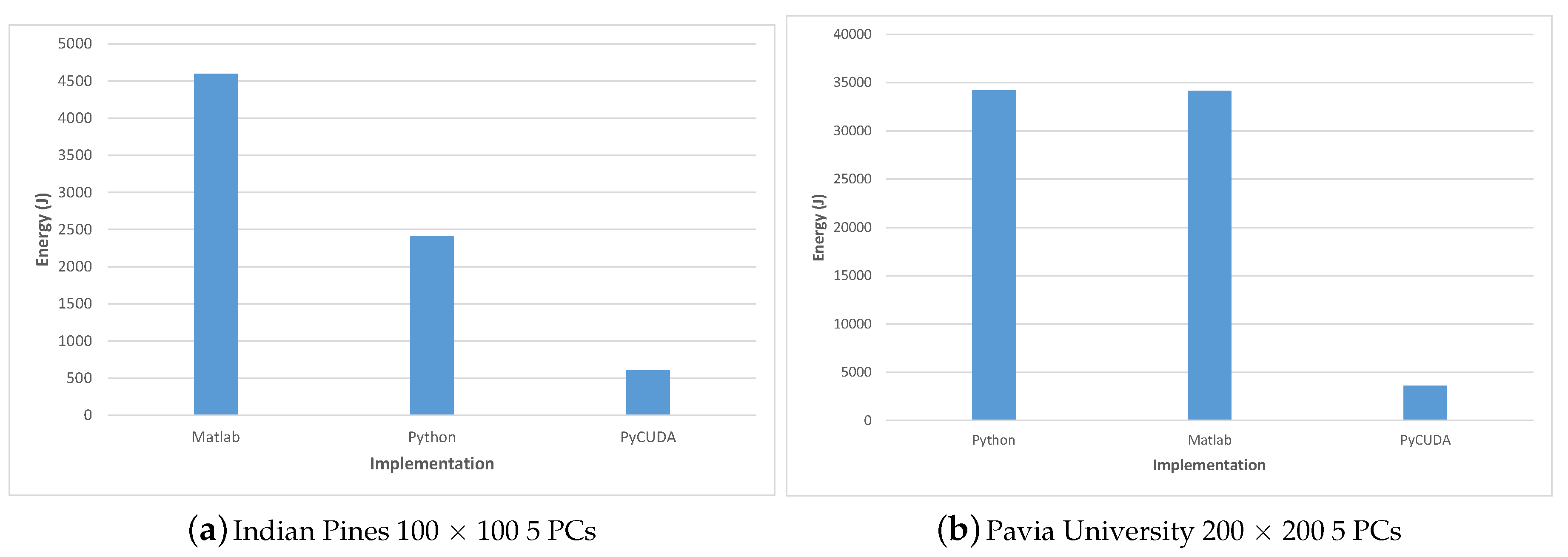
For evaluating the energy consumption we measured the system power consumption during the execution of each algorithm implementation for two test-cases: Indian Pines 100 × 100 and Pavia University 200 × 200; in all cases 5 PCs were computed. The system’s power consumption was measured using a PeakTech 1660 Digital Power Clamp Meter [46], which provides a USB connection and dedicated software for data acquisition, thus increasing the accuracy and reliability of the results.
The measurement results were consistent between the two test-cases and show on one hand that all parallel solutions consume much less total energy than the single-core implementation and on the other, that among all parallel implementation, the most efficient was the C++ MC AVX2 implementation, followed closely by the C++ MC CUDA implementation and the PyCUDA version.
Table 12 shows the energy consumption for the Matlab, Python and PyCUDA implementations versus the total execution time; the energy results are also displayed in Figure 15. Similarly, the energy consumption for the C++ implementations are illustrated in Table 13 and Figure 16.
C++ MC CUDA implementation is shown to be slightly less energy efficient than the C++ MC AVX2 implementation (consuming 24.74% more energy in the Indian Pines test-case and 4.89% more energy in the Pavia University test-case) but it outperforms the C++ MC AVX2 implementation in terms of execution speed (being 24.07% faster for the Indian Pines test-case and 39.89% faster for Pavia University). The difference in the increased energy consumption for the two test-cases (24.74% Indian Pines vs. 4.89% Pavia University) can be explained by the difference in the number of spectral bands (200 for Indian Pines vs. 103 for Pavia University), which leads to the number of threads per block being used by the CUDA kernel (256 for Indian Pines vs. 128 for Pavia University). These results are confirmed also in the case of the PyCUDA implementation, which uses the same CUDA kernel.
7. Conclusions
The recent trends and advances in remote sensing and Earth observation in recent years have led to the continuous acquisition of massive geospatial data of various formats. This raises scientific challenges related to the processing, analysis and visualization of remote sensing data, with focus on algorithms and computing paradigms able to extract knowledge and meaningful information both offline and in real time. Hence, the latest High Performance Computing devices and techniques, like parallel computing, GPUs and enhanced CPU instructions sets like AVX2 represent solutions able to provide significant gains in term of performance improvements of various data intensive applications and algorithms.
In this paper we have presented the implementation of a PP-based geometrical Principal Component Analysis approximation algorithm (gaPCA) for hyperspectral image analysis on a multi-core CPU, a GPU and multi-core CPU using AVX2 intrinsics, together with a comparative evaluation of the implementations in terms of execution time and energy consumption.
The experimental evaluation has shown that all parallel implementations have consistent speed-ups over the single core version: the C++ CUDA was on average 29.3× faster on Pavia and 24.8× faster on Indian Pines, while the C++ MC AVX2 version had an average speed-up of 21.2× for Pavia and 23.9× for Indian Pines compared to the baseline C++ SC version. These timing results show not only the advantage of using CUDA programming in implementing the gaPCA algorithm on a GPU in terms of performance and energy consumption, but also significant benefits in implementing it on the multi-core CPU using AVX2 intrinsics. These two implementations were shown to be much faster than the standard multi-core implementation, and also the most efficient with regard to energy consumption. The C++ MC AVX2 version was shown to be the most efficient, requiring on average 8.26× less energy when running the Pavia dataset and 9.71× less energy when running the Indian Pines dataset compared to the baseline C++ SC implementation. The C++ MC CUDA version had just slighlty lower results, being 7.88× more efficient on Pavia and 7.78× more efficient on Indian Pines than the single-core implementation.
Consequently, this paper highlights the benefits of using parallel computing, AVX2 intrinsics and CUDA parallel programming paradigms for accelerating dimensionality reduction algorithms like gaPCA in order to obtain significant speed-ups and improved energy efficiency over the traditional CPU single-core or multi-core implementations.
Author Contributions
Conceptualization, A.L.M. and O.M.M.; methodology, A.L.M. and C.B.C.; software, A.L.M.; validation, A.L.M., C.B.C., O.M.M. and P.L.O.; investigation, A.L.M. and O.M.M.; resources, O.M.M.; data curation, A.L.M.; writing—original draft preparation, A.L.M. and O.M.M.; writing—review and editing, C.B.C. and P.L.O.; visualization, A.L.M. and O.M.M.; supervision, P.L.O. All authors have read and agreed to the published version of the manuscript.
Funding
This research received no external funding.
Conflicts of Interest
The authors declare no conflict of interest.
Appendix A. Code Listings for gaPCA Parallel Implementations
Listing A1. Matlab implementation for the Euclidean distances function.
function [i_extreme, j_extreme, dist_max] euclidDist(X)
{
[m, n] = size(X);
parfor i = 1: m − 1
[d(i),j(i)] = max(pdist2(X(i,:),X(i + 1:m,:)));
end
[dist_max,ind] = max(d);
i_extreme = ind;
j_extreme = j(ind)+ind;
return
}
Listing A2. Python implementation for the Euclidean Distances function.
@jit(nopython = True, parallel = True, nogil = True)
def euclidDist(A):
dist = numpy.zeros(len(A))
index = numpy.zeros(len(A))
for i in prange(len(A) − 1):
temp_dist = numpy.zeros(len(A))
for j in prange(i + 1,len(A)):
temp_dist[j] = numpy.linalg.norm(A[i] − A[j])
dist[i] = numpy.amax(temp_dist)
index[i] = numpy.argmax(temp_dist)
return (numpy.amax(dist), numpy.argmax(dist), int(index[numpy.argmax(dist)]))
Listing A3. Pseudocode for the CUDA kernel computing pairwise Euclidean distance between the rows of the input matrix X.
euclidean kernel(input X, output C):
elem1 = X[blockIdx.x, threadIdx.y];
elem2 = X[blockIdx.y, threadIdx.y];
result = (elem1 − elem2)*(elem1 − elem2);
accum[threadIdx.y] = result;
Synchronize threads
Perform parallel tree-reduction and compute dist
if (dist>C[0])
C[0] = dist;
update indexes C[1] and C[2];
endif
Listing A4. CUDA kernel code for parallel tree-reduction.
__syncthreads();
//
for (int stride = SIZE/2; stride > 0; stride >>= 1) {
if (ty < stride)
accumResult[tx*SIZE + ty] += accumResult[stride + tx*SIZE+ty];
__syncthreads();
}
Listing A5. Source code for the C++ multi-core function computing pairwise Euclidean distances between the rows of the input matrix X.
void parallelDist(short **X, int n, int m, int& index1, int& index2, long long d)
{
long long dist[n] = { 0 };
int index[n] = { 0 };
#pragma omp parallel num_threads(12)
{
#pragma omp for
for (int i = 0; i < n −1; i++)
{
long long temp_dist[n] = {0};
for (int j = i + 1; j < n; j++)
{
temp_dist[j] = squarediff(m,X[i],X[j]);
}
dist[i] = *max_element(temp_dist,temp_dist + n);
index[i] = distance(temp_dist, max_element(temp_dist,temp_dist + n));
}
}
d = *max_element(dist, dist + n − 1);
index1 = distance(dist, max_element(dist,dist + n − 1));
index2 = index[index1];
}
Listing A6. Source code for the C++ alignment of a two-dimensional matrix of short.
alignas(__m256i) short **arr = (short **)malloc(ROWS * sizeof(short *));
std::size_t sz = COLS;
for (i = 0; i<ROWS; i++)
arr[i] = static_cast<short*>(aligned_alloc(32,sz*2));
Listing A7. Source code for the C++ SIMD function computing pairwise Euclidean distances.
long long squarediff_avx(int size, short *p1, short *p2)
{
std::size_t sz = size;
long long s = 0;
int i = 0;
for (; i + 16 <= size; i+ = 16 )
{
// load 256-bit chunks of each array
__m256i first_values = _mm256_load_si256((__m256i*) &p1[i]);
__m256i second_values = _mm256_load_si256((__m256i*) &p2[i]);
//substract each pair of 16-bit integers in the 256-bit chunks
__m256i substracted_values = _mm256_sub_epi16(first_values, second_values);
// multiply each pair of 16-bit integers in the 256-bit chunks
__m256i multiplied_values_lo = _mm256_mullo_epi16(substracted_values, substracted_values);
__m256i multiplied_values_hi = _mm256_mulhi_epi16(substracted_values, substracted_values);
s += sum_avx(multiplied_values_lo, multiplied_values_hi);
}
for (; i < size; i++)
{
s+= pow(p1[i] - p2[i],2);
}
return s;
}
Listing A8. Source code for the C++ multi-core function computing the sum of two 256-bit registers.
long long sum_avx(__m256i a_part1, __m256i a_part2)
}
short extracted_partial_sums1[16] = {0};
short extracted_partial_sums2[16] = {0};
_mm256_storeu_si256((__m256i*) &extracted_partial_sums1, a_part1);
_mm256_storeu_si256((__m256i*) &extracted_partial_sums2, a_part2);
long long sssum = 0;
for(int i = 0;i < 16;i++) }
int temp = ((extracted_partial_sums2[i]<<16) | ((extracted_partial_sums1[i]) & 0xffff));
sssum+=temp;
}
return sssum;
}
References
- Ali, A.; Qadir, J.; ur Rasool, R.; Sathiaseelan, A.; Zwitter, A.; Crowcroft, J. Big Data for Development: Applications and Techniques. Big Data Anal. 2016, 1, 2. [Google Scholar] [CrossRef] [Green Version]
- Campbell, J.B.; Wynne, R.H. Introduction to Remote Sensing; Guilford Press: New York, NY, USA, 2011. [Google Scholar]
- ESA: AVIRIS (Airborne Visible/Infrared Imaging Spectrometer). Available online: https://earth.esa.int/web/eoportal/airborne-sensors/aviris (accessed on 10 July 2019).
- Sorzano, C.O.S.; Vargas, J.; Montano, A.P. A Survey of Dimensionality Reduction Techniques. arXiv 2014, arXiv:1403.2877. [Google Scholar]
- van der Maaten, L.; Postma, E.O.; van den Herik, J. Dimensionality Reduction: A Comparative Review; BibSonomy: Wurzburg, Germany, 2009. [Google Scholar]
- Barcaru, A. Supervised Projection Pursuit—A Dimensionality Reduction Technique Optimized for Probabilistic Classification. Chemom. Intell. Lab. Syst. 2019, 194, 103867. [Google Scholar] [CrossRef]
- Friedman, J.H.; Tukey, J.W. A Projection Pursuit Algorithm for Exploratory Data Analysis. IEEE Trans. Comput. 1974, 100, 881–890. [Google Scholar] [CrossRef]
- Pearson, K. LIII. On lines and planes of closest fit to systems of points in space. Lond. Edinb. Dublin Philos. Mag. J. Sci. 1901, 2, 559–572. [Google Scholar] [CrossRef] [Green Version]
- Chang, C.I. Hyperspectral Data Processing: Algorithm Design and Analysis; John Wiley & Sons: Hoboken, NJ, USA, 2013. [Google Scholar]
- Lindholm, E.; Nickolls, J.; Oberman, S.; Montrym, J. NVIDIA Tesla: A Unified Graphics and Computing Architecture. IEEE Micro 2008, 28, 39–55. [Google Scholar] [CrossRef]
- Zhang, W.; Du, X.; Huang, A.; Yin, H. Analysis and Comprehensive Evaluation of Water Use Efficiency in China. Water 2019, 11, 2620. [Google Scholar] [CrossRef] [Green Version]
- Meehan, S.W.; Orlova, D.Y.; Moore, W.A.; Parks, D.R.; Meehan, C.; Walther, G.; Herzenberg, L.A. Fully Automated (Unsupervised) Identification, Matching, Display and Quantitation of Subsets (Clusters) by Exhaustive Projection Pursuit Methods. U.S. Patent App. 16/401,067, 28 November 2019. [Google Scholar]
- Lee, Y.D.; Cook, D.; Park, J.W.; Lee, E.K. PPtree: Projection pursuit classification tree. Electron. J. Stat. 2013, 7, 1369–1386. [Google Scholar] [CrossRef]
- Lee, E.K.; Cook, D.; Klinke, S.; Lumley, T. Projection pursuit for exploratory supervised classification. J. Comput. Graph. Stat. 2005, 14, 831–846. [Google Scholar] [CrossRef] [Green Version]
- Wang, L.; Wan, J.; Gao, X. Toward the Health Measure for Open Source Software Ecosystem Via Projection Pursuit and Real-Coded Accelerated Genetic. IEEE Access 2019, 7, 87396–87409. [Google Scholar] [CrossRef]
- Huang, W.; Zhang, X. Projection pursuit flood disaster classification assessment method based on multi-swarm cooperative particle swarm optimization. J. Water Resour. Prot. 2011, 3, 415. [Google Scholar] [CrossRef] [Green Version]
- YU, G.R.; YE, H.; XIA, Z.Q.; Zhao, X.Y. Improvement of Projection Pursuit Classification Model and Its Application in Evaluating Water Quality. J. Sichuan Univ. 2008, 6. [Google Scholar] [CrossRef]
- Ren, Y.; Liu, H.; Li, S.; Yao, X.; Liu, M. Prediction of binding affinities to β1 isoform of human thyroid hormone receptor by genetic algorithm and projection pursuit regression. Bioorganic Med. Chem. Lett. 2007, 17, 2474–2482. [Google Scholar] [CrossRef] [PubMed]
- Ren, Y.; Liu, H.; Yao, X.; Liu, M. Prediction of ozone tropospheric degradation rate constants by projection pursuit regression. Anal. Chim. Acta 2007, 589, 150–158. [Google Scholar] [CrossRef] [PubMed]
- Aladjem, M. Projection pursuit mixture density estimation. IEEE Trans. Signal Process. 2005, 53, 4376–4383. [Google Scholar] [CrossRef]
- Touboul, J. Projection pursuit through relative entropy minimization. Commun. Stat. Simul. Comput. 2011, 40, 854–878. [Google Scholar] [CrossRef] [Green Version]
- Bali, J.L.; Boente, G.; Tyler, D.E.; Wang, J.L. Robust functional principal components: A projection-pursuit approach. Ann. Stat. 2011, 39, 2852–2882. [Google Scholar] [CrossRef] [Green Version]
- Loperfido, N. Skewness-based projection pursuit: A computational approach. Comput. Stat. Data Anal. 2018, 120, 42–57. [Google Scholar] [CrossRef]
- Choulakian, V. L1-norm projection pursuit principal component analysis. Comput. Stat. Data Anal. 2006, 50, 1441–1451. [Google Scholar] [CrossRef]
- Jimenez, L.O.; Landgrebe, D. Projection pursuit for high dimensional feature reduction: Parallel and sequential approaches. In Proceedings of the 1995 International Geoscience and Remote Sensing Symposium, IGARSS’95. Quantitative Remote Sensing for Science and Applications, Firenze, Italy, 10–14 July 1995; Volume 1, pp. 148–150. [Google Scholar]
- Peña, D.; Prieto, F.J.; Viladomat, J. Eigenvectors of a kurtosis matrix as interesting directions to reveal cluster structure. J. Multivar. Anal. 2010, 101, 1995–2007. [Google Scholar] [CrossRef] [Green Version]
- Croux, C.; Ruiz-Gazen, A. High breakdown estimators for principal components: The projection-pursuit approach revisited. J. Multivar. Anal. 2005, 95, 206–226. [Google Scholar] [CrossRef] [Green Version]
- Grochowski, M.; Duch, W. Projection pursuit constructive neural networks based on quality of projected clusters. In Proceedings of the International Conference on Artificial Neural Networks, Prague, Czech Republic, 3–6 September 2008; pp. 754–762. [Google Scholar]
- Grochowski, M.; Duch, W. Fast projection pursuit based on quality of projected clusters. In Proceedings of the International Conference on Adaptive and Natural Computing Algorithms, Ljubljana, Slovenia, 14–16 April 2011; pp. 89–97. [Google Scholar]
- Hui, G.; Lindsay, B.G. Projection pursuit via white noise matrices. Sankhya B 2010, 72, 123–153. [Google Scholar] [CrossRef]
- Kwatra, V.; Han, M. Fast Covariance Computation and Dimensionality Reduction for Sub-window Features in Images. In Proceedings of the 11th European Conference on Computer Vision: Part II, Crete, Greece, 5–11 September 2010; Springer: Berlin/Heidelberg, Germany, 2010; pp. 156–169. [Google Scholar]
- Funatsu, N.; Kuroki, Y. Fast Parallel Processing using GPU in Computing L1-PCA Bases. In Proceedings of the TENCON 2010–2010 IEEE Region 10 Conference, Fukuoka, Japan, 21–24 November 2010; pp. 2087–2090. [Google Scholar]
- Jošth, R.; Antikainen, J.; Havel, J.; Herout, A.; Zemčík, P.; Hauta-Kasari, M. Real-time PCA calculation for spectral imaging (using SIMD and GP-GPU). J. Real Time Image Process. 2012, 7, 95–103. [Google Scholar] [CrossRef]
- Andrecut, M. Parallel GPU implementation of iterative PCA algorithms. J. Comput. Biol. 2009, 16, 1593–1599. [Google Scholar] [CrossRef] [Green Version]
- Melikyan, V.S.; Osipyan, H. Modified fast PCA algorithm on GPU architecture. In Proceedings of the IEEE East-West Design & Test Symposium (EWDTS 2014), Kiev, Ukraine, 26–29 September 2014; pp. 1–4. [Google Scholar]
- Antikainen, J.; Hauta-Kasari, M.; Jaaskelainen, T.; Parkkinen, J. Fast Non-Iterative PCA computation for spectral image analysis using GPU. In Proceedings of the Conference on Colour in Graphics, Imaging, and Vision. Society for Imaging Science and Technology, Joensuu, Finland, 14–17 June 2010; Volume 2010, pp. 554–559. [Google Scholar]
- Lazcano, R.; Madroñal, D.; Fabelo, H.; Ortega, S.; Salvador, R.; Callicó, G.M.; Juárez, E.; Sanz, C. Parallel implementation of an iterative PCA algorithm for hyperspectral images on a manycore platform. In Proceedings of the 2017 Conference on Design and Architectures for Signal and Image Processing (DASIP), Dresden, Germany, 27–29 September 2017; pp. 1–6. [Google Scholar]
- Lazcano, R.; Madroñal, D.; Fabelo, H.; Ortega, S.; Salvador, R.; Callico, G.; Juarez, E.; Sanz, C. Adaptation of an iterative PCA to a manycore architecture for hyperspectral image processing. J. Signal Process. Syst. 2019, 91, 759–771. [Google Scholar] [CrossRef]
- Martel, E.; Lazcano, R.; López, J.; Madroñal, D.; Salvador, R.; López, S.; Juarez, E.; Guerra, R.; Sanz, C.; Sarmiento, R. Implementation of the Principal Component Analysis onto High-Performance Computer facilities for hyperspectral dimensionality reduction: Results and comparisons. Remote Sens. 2018, 10, 864. [Google Scholar] [CrossRef] [Green Version]
- Fernandez, D.; Gonzalez, C.; Mozos, D.; Lopez, S. FPGA implementation of the Principal Component Analysis algorithm for dimensionality reduction of hyperspectral images. J. Real Time Image Process. 2016. [Google Scholar] [CrossRef]
- Du, H.; Qi, H. An FPGA implementation of parallel ICA for dimensionality reduction in hyperspectral images. In Proceedings of the IGARSS 2004. 2004 IEEE International Geoscience and Remote Sensing Symposium, Anchorage, AK, USA, 20–24 September 2004; Volume 5, pp. 3257–3260. [Google Scholar]
- Mansoori, M.A.; Casu, M.R. Efficient FPGA Implementation of PCA Algorithm for Large Data using High Level Synthesis. In Proceedings of the 2019 15th Conference on Ph. D Research in Microelectronics and Electronics (PRIME), Lausanne, Switzerland, 15–18 July 2019; pp. 65–68. [Google Scholar]
- Wu, Z.; Li, Y.; Plaza, A.; Li, J.; Xiao, F.; Wei, Z. Parallel and distributed dimensionality reduction of hyperspectral data on cloud computing architectures. IEEE J. Sel. Top. Appl. Earth Obs. Remote. Sens. 2016, 9, 2270–2278. [Google Scholar] [CrossRef]
- AMD Ryzen 5 3600 Processor Specifications. Available online: https://www.amd.com/en/products/cpu/amd-ryzen-5-3600 (accessed on 17 September 2019).
- GeForce GTX 1650. Available online: https://www.nvidia.com/ro-ro/geforce/graphics-cards/gtx-1650/ (accessed on 17 September 2019).
- Peaktech. Available online: https://www.peaktech.de/productdetail/kategorie/digital-leistungszangenmessgeraet/produkt/peaktech-1660.html/ (accessed on 24 January 2020).
- Pavia University Hyperspectral Remote Sensing Scene. Available online: http://www.ehu.eus/ccwintco/index.php/Hyperspectral_Remote_Sensing_Scenes#Pavia_University (accessed on 7 August 2019).
- Indian Pines Hyperspectral Remote Sensing Scene. Available online: http://www.ehu.eus/ccwintco/index.php/Hyperspectral_Remote_Sensing_Scenes#Indian_Pines (accessed on 7 August 2019).
- Machidon, A.L.; Ciobanu, C.B.; Machidon, O.M.; Ogrutan, P.L. On Parallelizing Geometrical PCA Approximation. In Proceedings of the 2019 18th RoEduNet Conference: Networking in Education and Research (RoEduNet), Galați, Romania, 10–12 October 2019; pp. 1–6. [Google Scholar]
- Härdle, W.; Klinke, S.; Turlach, B.A. XploRe: An Interactive Statistical Computing Environment; Springer Science & Business Media: Berlin/Heidelberg, Germany, 2012. [Google Scholar]
- Dayal, M. A New Algorithm for Exploratory Projection Pursuit. arXiv 2018, arXiv:1112.4321. [Google Scholar]
- Ifarraguerri, A.; Chang, C.I. Unsupervised hyperspectral image analysis with projection pursuit. IEEE Trans. Geosci. Remote Sens. 2000, 38, 2529–2538. [Google Scholar]
- Machidon, A.; Coliban, R.; Machidon, O.; Ivanovici, M. Maximum Distance-based PCA Approximation for Hyperspectral Image Analysis and Visualization. In Proceedings of the 2018 41st International Conference on Telecommunications and Signal Processing (TSP), Athens, Greece, 4–6 July 2018. [Google Scholar] [CrossRef]
- Machidon, A.L.; Machidon, O.M.; Ogrutan, P.L. Face Recognition Using Eigenfaces, Geometrical PCA Approximation and Neural Networks. In Proceedings of the 2019 42nd International Conference on Telecommunications and Signal Processing (TSP), Budapest, Hungary, 3–5 July 2019; pp. 80–83. [Google Scholar] [CrossRef]
- Machidon, A.L.; Del Frate, F.; Picchiani, M.; Machidon, O.M.; Ogrutan, P.L. Geometrical Approximated Principal Component Analysis for Hyperspectral Image Analysis. Remote Sens. 2020, 12, 1698. [Google Scholar] [CrossRef]
- ENVI Image Analysis Software. Available online: https://www.harrisgeospatial.com/Software-Technology/ENVI (accessed on 24 April 2020).
- McNemar, Q. Note on the sampling error of the difference between correlated proportions or percentages. Psychometrika 1947, 12, 153–157. [Google Scholar] [CrossRef] [PubMed]
- PyCUDA. Available online: https://mathema.tician.de/software/pycuda/ (accessed on 19 August 2019).
- Python. Available online: https://www.python.org/ (accessed on 1 August 2019).
- Numba. Available online: https://numba.pydata.org/ (accessed on 1 August 2019).
- LLVM. Available online: https://llvm.org/ (accessed on 22 January 2019).
- OpenMP. Available online: https://www.openmp.org/ (accessed on 19 December 2019).
- Peleg, A.; Weiser, U. MMX technology extension to the Intel architecture. IEEE Micro 1996, 16, 42–50. [Google Scholar] [CrossRef]
- Raman, S.K.; Pentkovski, V.; Keshava, J. Implementing streaming SIMD extensions on the Pentium III processor. IEEE Micro 2000, 20, 47–57. [Google Scholar] [CrossRef]
- Lomont, C. Introduction to intel advanced vector extensions. Intel White Pap. 2011, 23. [Google Scholar]
- avx2. Available online: https://software.intel.com/en-us/cpp-compiler-developer-guide-and-reference-overview-intrinsics-for-intel-advanced-vector-extensions-2-intel-avx2-instructions/ (accessed on 22 January 2019).
- Kukunas, J. Power and Performance: Software Analysis and Optimization; Morgan Kaufmann: San Francisco, CA, USA, 2015. [Google Scholar]
- Luo, Y.; John, L.K.; Eeckhout, L. Self-monitored adaptive cache warm-up for microprocessor simulation. In Proceedings of the 16th Symposium on Computer Architecture and High Performance Computing, Foz Do Iguacu, Brazil, 27–29 October 2004; pp. 10–17. [Google Scholar] [CrossRef]
Figure 1.
RGB visualisation of the two hyperspectral datasets used for experiments, Pavia University (a) and Indian Pines (b).
Figure 1.
RGB visualisation of the two hyperspectral datasets used for experiments, Pavia University (a) and Indian Pines (b).
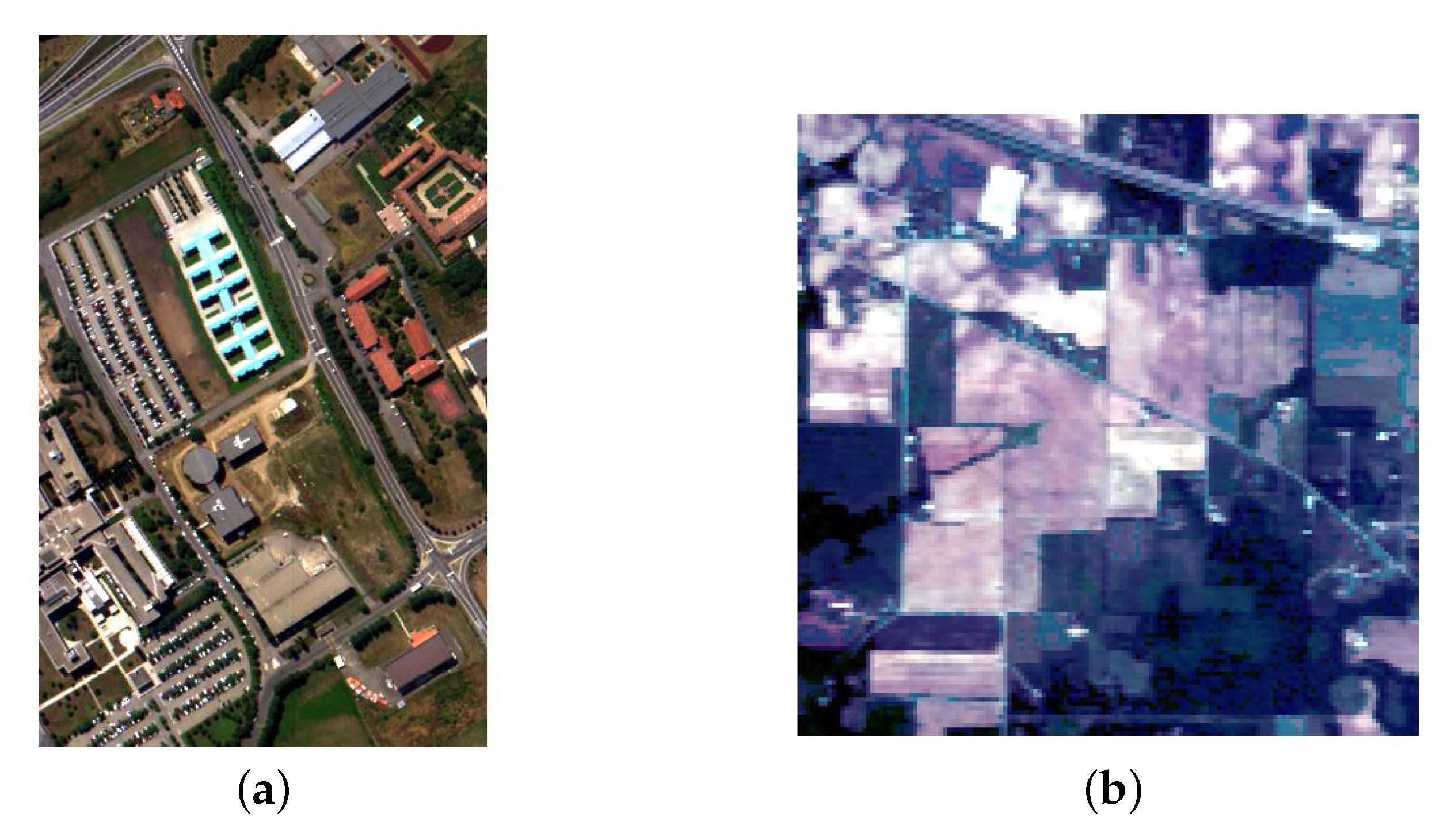
Figure 2.
Geometrical approximated Principal Component Analysis (gaPCA) Principal Components (green) vs. canonical PCA Principal Components (magenta) computed on a correlated 2D point cloud.
Figure 2.
Geometrical approximated Principal Component Analysis (gaPCA) Principal Components (green) vs. canonical PCA Principal Components (magenta) computed on a correlated 2D point cloud.

Figure 3.
Standard PCA (a) and gaPCA (b) images classified (Maximum Likelihood) vs. the groundtruth image (c) of the Indian Pines dataset.
Figure 3.
Standard PCA (a) and gaPCA (b) images classified (Maximum Likelihood) vs. the groundtruth image (c) of the Indian Pines dataset.

Figure 4.
Standard PCA (a) and gaPCA (b) images classified (Maximum Likelihood) vs. the groundtruth (c) of the Pavia University dataset.
Figure 4.
Standard PCA (a) and gaPCA (b) images classified (Maximum Likelihood) vs. the groundtruth (c) of the Pavia University dataset.

Figure 5.
Diagram showing gaPCA algorithm design and the two sub-routines with parallel implementations.
Figure 5.
Diagram showing gaPCA algorithm design and the two sub-routines with parallel implementations.

Figure 6.
Diagram showing one iteration of the Euclidean distances function.
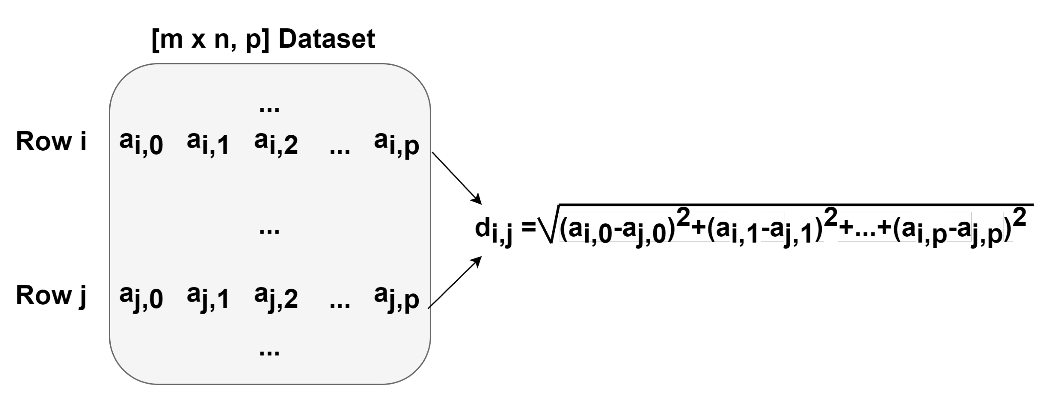
Figure 7.
Diagram showing the parallel implementation in Compute Unified Device Architecture (CUDA) of the Euclidean distance function.
Figure 7.
Diagram showing the parallel implementation in Compute Unified Device Architecture (CUDA) of the Euclidean distance function.

Figure 8.
Indian Pines Matlab vs.Python vs. PyCUDA speedup for 1 PC (a), 3 PCs (b) and 5 PC (c) for various image dimensions.
Figure 8.
Indian Pines Matlab vs.Python vs. PyCUDA speedup for 1 PC (a), 3 PCs (b) and 5 PC (c) for various image dimensions.

Figure 9.
Pavia University Matlab vs. Python vs. PyCUDA speedup for 1 PC (a), 3 PCs (b) and 5 PC (c) for various image dimensions.
Figure 9.
Pavia University Matlab vs. Python vs. PyCUDA speedup for 1 PC (a), 3 PCs (b) and 5 PC (c) for various image dimensions.
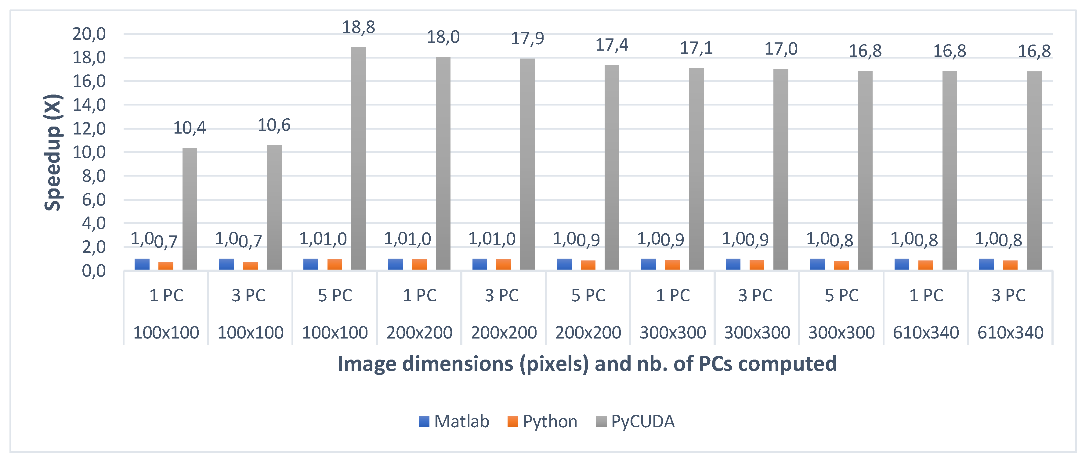
Figure 10.
Indian Pines C++ Single Core (SC) vs. Single Core AVX2 (SC AVX2) vs. Multi Core (MC) vs. Multi Core AVX2 (MC AVX2) speedup for 1 PC (a), 3 PCs (b) and 5 PC (c) for various image dimensions.
Figure 10.
Indian Pines C++ Single Core (SC) vs. Single Core AVX2 (SC AVX2) vs. Multi Core (MC) vs. Multi Core AVX2 (MC AVX2) speedup for 1 PC (a), 3 PCs (b) and 5 PC (c) for various image dimensions.
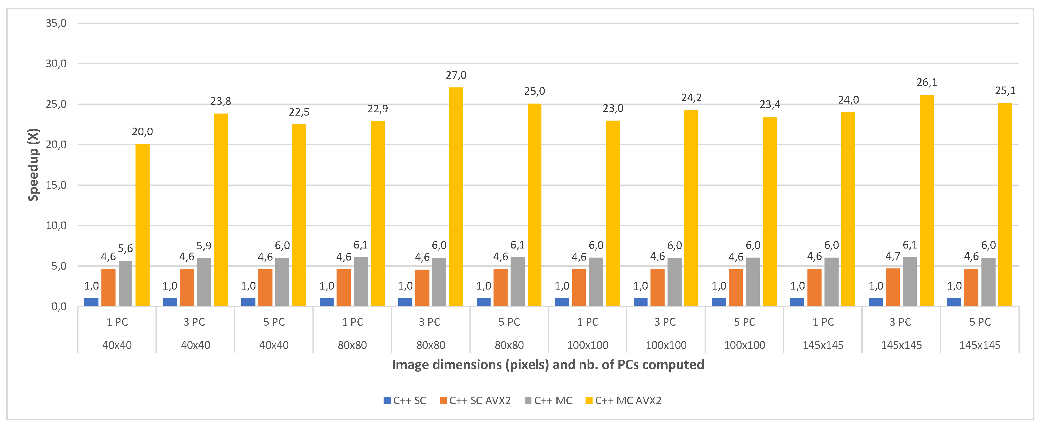
Figure 11.
Pavia University C++ Single Core (SC) vs. Single Core AVX2 (SC AVX2) vs. Multi Core (MC) vs. Multi Core AVX2 (MC AVX2) speedup for 1 PC (a), 3 PCs (b) and 5 PC (c) for various image dimensions.
Figure 11.
Pavia University C++ Single Core (SC) vs. Single Core AVX2 (SC AVX2) vs. Multi Core (MC) vs. Multi Core AVX2 (MC AVX2) speedup for 1 PC (a), 3 PCs (b) and 5 PC (c) for various image dimensions.

Figure 12.
Indian Pines C++ Multi Core (MC) vs. Multi Core AVX2 (MC AVX2) vs. Multi Core CUDA (MC CUDA) speedup for 1 PC (a) 3 PCs, (b) and 5 PC (c) for various image dimensions.
Figure 12.
Indian Pines C++ Multi Core (MC) vs. Multi Core AVX2 (MC AVX2) vs. Multi Core CUDA (MC CUDA) speedup for 1 PC (a) 3 PCs, (b) and 5 PC (c) for various image dimensions.
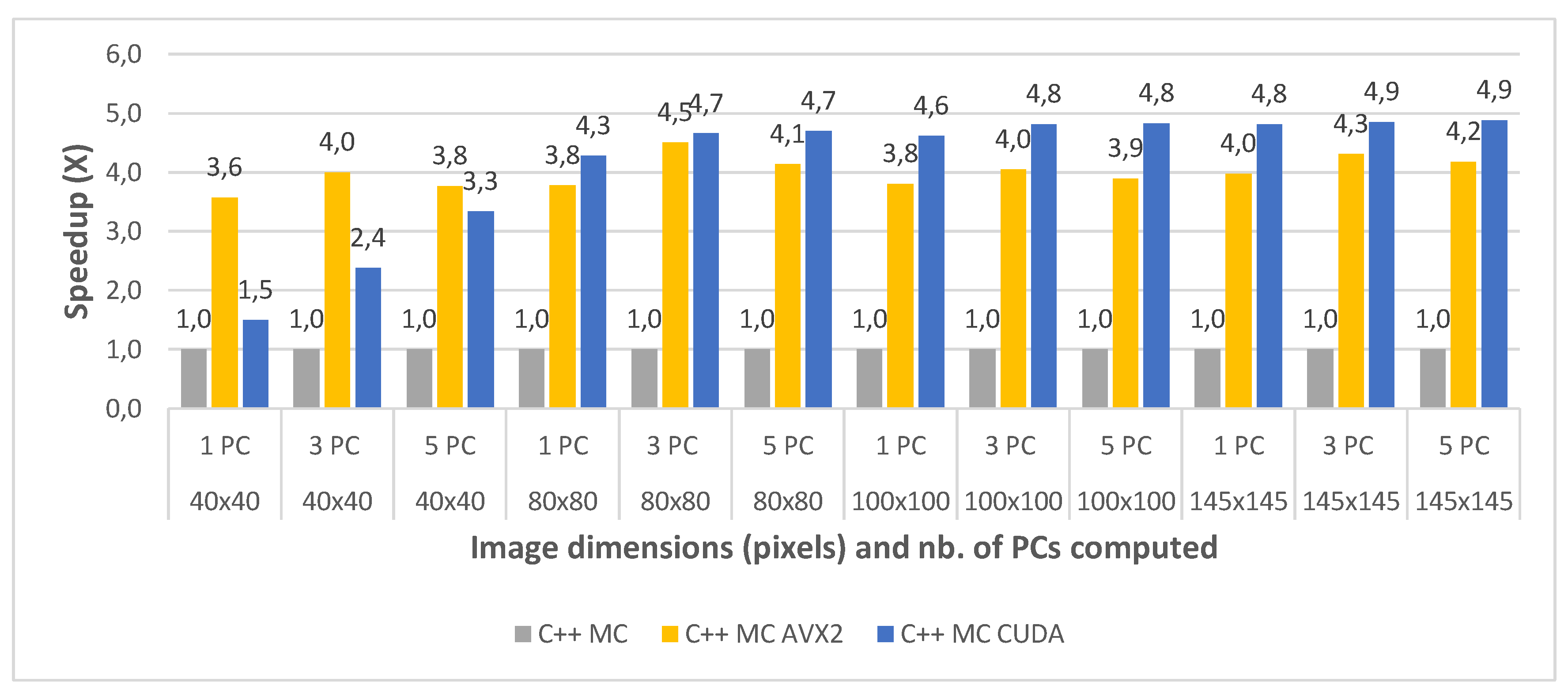
Figure 13.
Pavia University C++ Multi Core (MC) vs. Multi Core AVX2 (MC AVX2) vs. Multi Core CUDA (MC CUDA) speedup for 1 PC (a) 3 PCs, (b) and 5 PC (c) for various image dimensions.
Figure 13.
Pavia University C++ Multi Core (MC) vs. Multi Core AVX2 (MC AVX2) vs. Multi Core CUDA (MC CUDA) speedup for 1 PC (a) 3 PCs, (b) and 5 PC (c) for various image dimensions.
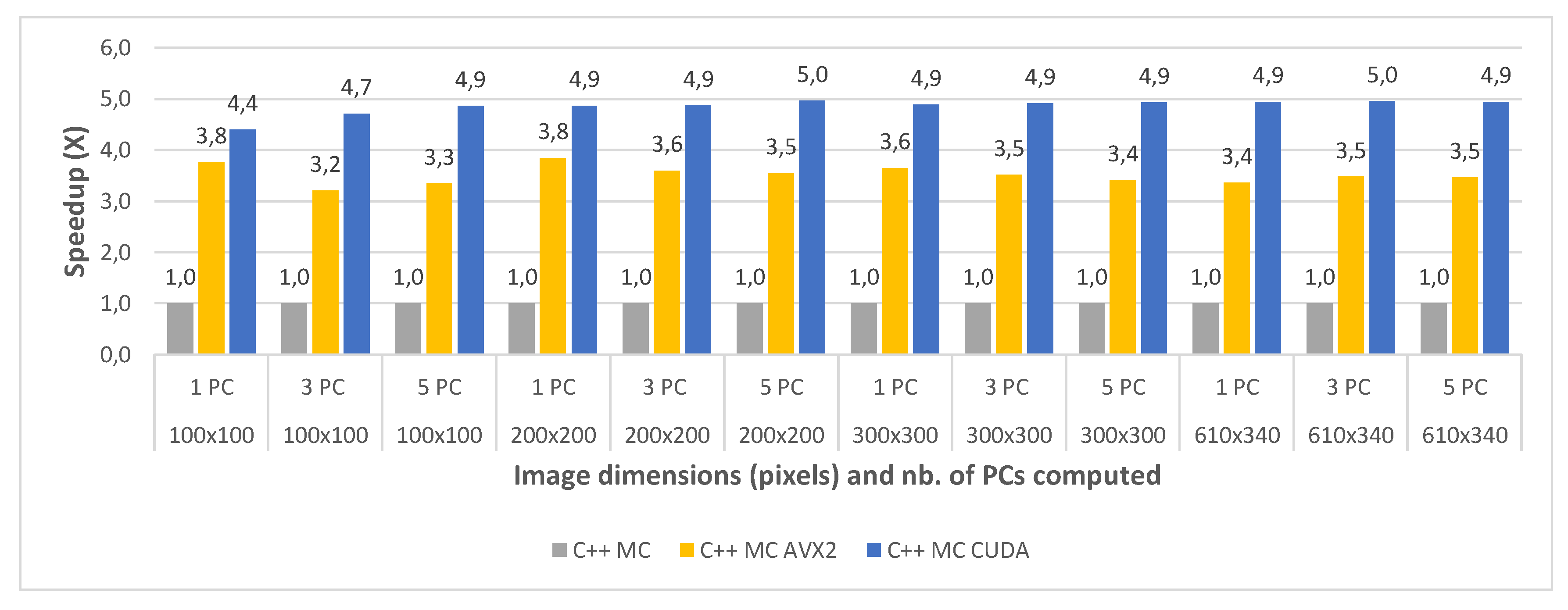
Figure 14.
gaPCA overall speedup comparison.

Figure 15.
Energy consumption for the Indian Pines (a) and Pavia University (b) datasets for the Matlab, Python and PyCUDA implementations.
Figure 15.
Energy consumption for the Indian Pines (a) and Pavia University (b) datasets for the Matlab, Python and PyCUDA implementations.

Figure 16.
Energy consumption for the Indian Pines (a) and Pavia University (b) datasets for the C++ implementations.
Figure 16.
Energy consumption for the Indian Pines (a) and Pavia University (b) datasets for the C++ implementations.

Table 1.
AMD Ryzen 5 3600 CPU specifications.
| Proccesor | AMD Ryzen 5 3600 |
|---|---|
| Cores | 6 |
| Threads | 12 |
| Base Clock | 3.6 GHz |
| Maximum Boost Clock | 4.2 GHz |
| Memory | 384KB L1, 3MB L2, 32MB L3 |
Table 2.
GeForce GTX 1650 specifications.
| GPU | GeForce GTX 1650 |
|---|---|
| CUDA Cores | 896 |
| Processor Base Clock | 1485 MHz |
| Processor Max Boost Clock | 1665 MHz |
| Memory | 4GB GDDR5 |
| Memory Bandwidth | 128 GB/s |
Table 3.
Classification results for the Indian Pines dataset.
| Class | Training Pixels | PCA ML | gaPCA ML | PCA SVM | gaPCA SVM |
|---|---|---|---|---|---|
| Alfalfa | 32 | 98.7 | 80.5 | 18.2 | 18.2 |
| Corn notill | 1145 | 30.6 | 47.6 | 65.2 | 69.3 |
| Corn mintill | 595 | 51.6 | 69.2 | 34.9 | 46.1 |
| Corn | 167 | 84.9 | 100 | 31.4 | 37.7 |
| Grass pasture | 328 | 55.7 | 80.5 | 64.6 | 71.9 |
| Grass trees | 463 | 96.1 | 90.6 | 91.2 | 92.5 |
| Grass pasture mowed | 19 | 68.3 | 71.7 | 60 | 60 |
| Hay windrowed | 528 | 88.5 | 96.7 | 99.5 | 99.6 |
| Oats | 20 | 100 | 96.9 | 15.6 | 6.3 |
| Soybean notill | 681 | 83.7 | 77.1 | 40.9 | 56.1 |
| Soybean mintill | 1831 | 46.6 | 47.7 | 79.4 | 78.3 |
| Soybean clean | 457 | 36.9 | 77.7 | 11.8 | 36.1 |
| Wheat | 150 | 97.2 | 97 | 91.1 | 93.1 |
| Woods | 884 | 98.7 | 96.9 | 97.3 | 97.3 |
| Buildings Drives | 263 | 33.7 | 61.4 | 45.5 | 52.1 |
| Stone Steel Towers | 103 | 100 | 100 | 95.5 | 97.2 |
| zML = 25.1 (signif = yes) | OA(%) | 62.1 | 70.2 | 67.2 | 72.1 |
| zSVM = 24.8 (signif = yes) | Kappa | 0.57 | 0.67 | 0.62 | 0.68 |
Table 4.
Classification results for the Pavia University dataset.
| Class | Training Pixels | PCA ML | gaPCA ML | PCA SVM | gaPCA SVM |
|---|---|---|---|---|---|
| Asphalt (grey) | 1766 | 60.5 | 61.5 | 67.2 | 78.3 |
| Meadows (light green) | 2535 | 68.3 | 80 | 65 | 86.9 |
| Gravel (cyan) | 923 | 100 | 100 | 33.3 | 40 |
| Trees (dark green) | 599 | 88.2 | 89.7 | 100 | 67.7 |
| Metal sheets (magenta) | 872 | 100 | 100 | 100 | 100 |
| Bare soil (brown) | 1579 | 77.8 | 79.4 | 53.2 | 68.3 |
| Bitumen (purple) | 565 | 89.7 | 89.7 | 89.7 | 55.2 |
| Bricks (red) | 1474 | 68.3 | 72 | 81.7 | 86.6 |
| Shadows (yellow) | 876 | 100 | 100 | 100 | 100 |
| zML = 4.87 (signif = yes) | OA(%) | 72.2 | 78 | 69 | 78 |
| zSVM = 5.97 (signif = yes) | Kappa | 0.65 | 0.72 | 0.61 | 0.72 |
Table 5.
Excerpt from the confusion matrix for the Pavia University dataset.
| Class | True | False |
|---|---|---|
| Asphalt (PCA) | 60.5 Asphalt | 29.5 Bitumen |
| Asphalt (gaPCA) | 61.5 Asphalt | 21.8 Bitumen |
| Meadows (PCA) | 68.3 Meadows | 25.8 Bare soil |
| Meadows (gaPCA) | 80 Meadows | 17.6 Bare soil |
| Bricks (PCA) | 68.3 Bricks | 25.6 Gravel |
| Bricks (gaPCA) | 72 Bricks | 24.3 Gravel |
Table 6.
Indian Pines Matlab vs. Python vs. PyCUDA execution times (s).
| Crop Size | No. of PCs | Matlab | Python | PyCUDA |
|---|---|---|---|---|
| 40 × 40 | 1 | 0.275 | 1.260 | 0.153 |
| 40 × 40 | 3 | 0.832 | 2.802 | 0.449 |
| 40 × 40 | 5 | 1.448 | 3.519 | 0.756 |
| 80 × 80 | 1 | 8.326 | 6.797 | 0.769 |
| 80 × 80 | 3 | 24.678 | 18.265 | 2.319 |
| 80 × 80 | 5 | 40.990 | 29.333 | 3.884 |
| 100 × 100 | 1 | 22.090 | 14.531 | 1.592 |
| 100 × 100 | 3 | 66.377 | 41.929 | 4.843 |
| 100 × 100 | 5 | 110.449 | 68.647 | 8.004 |
| 145 × 145 | 1 | 104.134 | 64.498 | 5.843 |
| 145 × 145 | 3 | 313.070 | 181.152 | 18.036 |
| 145 × 145 | 5 | 521.057 | 298.212 | 30.137 |
Table 7.
Pavia University Matlab vs. Python vs. PyCUDA execution times (s).
| Crop Size | No. of PCs | Matlab | Python | PyCUDA |
|---|---|---|---|---|
| 100 × 100 | 1 | 9.507 | 13.476 | 0.866 |
| 100 × 100 | 3 | 28.439 | 39.126 | 2.745 |
| 100 × 100 | 5 | 47.580 | 64.131 | 4.497 |
| 200 × 200 | 1 | 195.801 | 204.855 | 10.391 |
| 200 × 200 | 3 | 575.083 | 601.477 | 31.884 |
| 200 × 200 | 5 | 957.494 | 992.193 | 53.496 |
| 300 × 300 | 1 | 883.342 | 1027.397 | 50.905 |
| 300 × 300 | 3 | 2653.649 | 3036.512 | 155.068 |
| 300 × 300 | 5 | 4432.107 | 5030.831 | 260.203 |
| 610 × 340 | 1 | 4501.181 | 5453.752 | 267.402 |
| 610 × 340 | 3 | 13,588.632 | 16,035.242 | 806.866 |
| 610 × 340 | 5 | 22,675.191 | 26,702.160 | 1347.312 |
Table 8.
Indian Pines C++ Single Core (SC) vs. Single Core AVX2 (SC AVX2) vs. Multi Core (MC) vs. Multi Core AVX2 (MC AVX2) execution times (s).
Table 8.
Indian Pines C++ Single Core (SC) vs. Single Core AVX2 (SC AVX2) vs. Multi Core (MC) vs. Multi Core AVX2 (MC AVX2) execution times (s).
| Crop Size | No. of PCs | C++ SC | C++ SC AVX2 | C++ MC | C++ MC AVX2 |
|---|---|---|---|---|---|
| 40 × 40 | 1 | 0.947 | 0.206 | 0.169 | 0.047 |
| 40 × 40 | 3 | 2.858 | 0.620 | 0.480 | 0.120 |
| 40 × 40 | 5 | 4.749 | 1.035 | 0.796 | 0.211 |
| 80 × 80 | 1 | 15.147 | 3.317 | 2.502 | 0.663 |
| 80 × 80 | 3 | 45.274 | 9.942 | 7.534 | 1.674 |
| 80 × 80 | 5 | 75.451 | 16.389 | 12.457 | 3.012 |
| 100 × 100 | 1 | 36.834 | 8.070 | 6.108 | 1.605 |
| 100 × 100 | 3 | 110.570 | 23.834 | 18.452 | 4.560 |
| 100 × 100 | 5 | 184.189 | 40.409 | 30.627 | 7.871 |
| 145 × 145 | 1 | 162.853 | 35.185 | 27.017 | 6.797 |
| 145 × 145 | 3 | 491.379 | 105.084 | 81.027 | 18.816 |
| 145 × 145 | 5 | 814.208 | 175.127 | 135.510 | 32.400 |
Table 9.
Pavia University C++ Single Core (SC) vs. Single Core AVX2 (SC AVX2) vs. Multi Core (MC) vs. Multi Core AVX2 (MC AVX2) execution times (s).
Table 9.
Pavia University C++ Single Core (SC) vs. Single Core AVX2 (SC AVX2) vs. Multi Core (MC) vs. Multi Core AVX2 (MC AVX2) execution times (s).
| Crop Size | No. of PCs | C++ SC | C++ SC AVX2 | C++ MC | C++ MC AVX2 |
|---|---|---|---|---|---|
| 100 × 100 | 1 | 18.373 | 4.63084 | 3.030 | 0.805 |
| 100 × 100 | 3 | 55.185 | 13.9219 | 9.025 | 2.814 |
| 100 × 100 | 5 | 91.666 | 23.1688 | 15.277 | 4.565 |
| 200 × 200 | 1 | 293.311 | 74.8406 | 48.650 | 12.652 |
| 200 × 200 | 3 | 880.324 | 222.279 | 144.703 | 40.199 |
| 200 × 200 | 5 | 1472.080 | 371.005 | 243.616 | 68.642 |
| 300 × 300 | 1 | 1488.370 | 387.629 | 247.666 | 67.894 |
| 300 × 300 | 3 | 4489.640 | 1165.61 | 741.890 | 211.110 |
| 300 × 300 | 5 | 7438.200 | 1933.44 | 1240.140 | 363.606 |
| 610 × 340 | 1 | 7956.360 | 2053.12 | 1322.530 | 393.734 |
| 610 × 340 | 3 | 23,962.794 | 6202.35 | 3975.840 | 1144.730 |
| 610 × 340 | 5 | 40,190.385 | 10,408.8 | 6605.060 | 1905.980 |
Table 10.
Indian Pines C++ Multi Core (MC) vs. Multi Core AVX2 (MC AVX2) vs. Multi Core CUDA (MC CUDA) execution times (s).
Table 10.
Indian Pines C++ Multi Core (MC) vs. Multi Core AVX2 (MC AVX2) vs. Multi Core CUDA (MC CUDA) execution times (s).
| Crop Size | No. of PCs | C++ MC | C++ MC AVX2 | C++ MC CUDA |
|---|---|---|---|---|
| 40 × 40 | 1 | 0.169 | 0.047 | 0.113 |
| 40 × 40 | 3 | 0.480 | 0.120 | 0.202 |
| 40 × 40 | 5 | 0.796 | 0.211 | 0.239 |
| 80 × 80 | 1 | 2.502 | 0.663 | 0.585 |
| 80 × 80 | 3 | 7.534 | 1.674 | 1.619 |
| 80 × 80 | 5 | 12.457 | 3.012 | 2.654 |
| 100 × 100 | 1 | 6.108 | 1.605 | 1.324 |
| 100 × 100 | 3 | 18.452 | 4.560 | 3.835 |
| 100 × 100 | 5 | 30.627 | 7.871 | 6.343 |
| 145 × 145 | 1 | 27.017 | 6.797 | 5.609 |
| 145 × 145 | 3 | 81.027 | 18.816 | 16.690 |
| 145 × 145 | 5 | 135.510 | 32.400 | 27.770 |
Table 11.
Pavia University C++ Multi Core (MC) vs. Multi Core AVX2 (MC AVX2) vs. Multi Core CUDA (MC CUDA) execution times (s).
Table 11.
Pavia University C++ Multi Core (MC) vs. Multi Core AVX2 (MC AVX2) vs. Multi Core CUDA (MC CUDA) execution times (s).
| Crop Size | No. of PCs | C++ MC | C++ MC AVX2 | C++ MC CUDA |
|---|---|---|---|---|
| 100 × 100 | 1 | 3.030 | 0.805 | 0.689 |
| 100 × 100 | 3 | 9.025 | 2.814 | 1.916 |
| 100 × 100 | 5 | 15.277 | 4.565 | 3.143 |
| 200 × 200 | 1 | 48.650 | 12.652 | 9.989 |
| 200 × 200 | 3 | 144.703 | 40.199 | 29.699 |
| 200 × 200 | 5 | 243.616 | 68.642 | 49.068 |
| 300 × 300 | 1 | 247.666 | 67.894 | 50.700 |
| 300 × 300 | 3 | 741.890 | 211.110 | 151.082 |
| 300 × 300 | 5 | 1240.140 | 363.606 | 251.730 |
| 610 × 340 | 1 | 1322.530 | 393.734 | 267.495 |
| 610 × 340 | 3 | 3975.840 | 1144.730 | 801.950 |
| 610 × 340 | 5 | 6605.060 | 1905.980 | 1336.010 |
Table 12.
Energy measurement results for the Matlab, Python and PyCUDA implementations.
| Dataset | Size | No. of PCs | Implementation | Energy (J) | Time (s) |
|---|---|---|---|---|---|
| Indian | 100 × 100 | 5 | Matlab | 4595.29 | 110.449 |
| Python | 2409.06 | 68.647 | |||
| PyCUDA | 609.23 | 8.004 | |||
| Pavia U | 200 × 200 | 5 | Matlab | 34,139.77 | 957.494 |
| Python | 34,192.04 | 992.193 | |||
| PyCUDA | 3589.8 | 53.496 |
Table 13.
Energy measurement results for the C++ implementations.
| Dataset | Size | No. of PCs | Implementation | Energy (J) | Time (s) |
|---|---|---|---|---|---|
| Indian | 100 × 100 | 5 | C++ SC | 3672 | 184.189 |
| C++ MC | 1108.75 | 30.627 | |||
| C++ SC AVX2 | 792 | 40.409 | |||
| C++ MC CUDA | 471.43 | 6.343 | |||
| C++ MC AVX2 | 378 | 7.871 | |||
| Pavia U | 200 × 200 | 5 | C++ SC | 27,512.87 | 1472.080 |
| C++ MC | 9242.40 | 243.616 | |||
| C++ SC AVX2 | 7431.87 | 371.005 | |||
| C++ MC CUDA | 3491.43 | 49.068 | |||
| C++ MC AVX2 | 3328.63 | 68.642 |
© 2020 by the authors. Licensee MDPI, Basel, Switzerland. This article is an open access article distributed under the terms and conditions of the Creative Commons Attribution (CC BY) license (http://creativecommons.org/licenses/by/4.0/).
Share and Cite
MDPI and ACS Style
Machidon, A.L.; Machidon, O.M.; Ciobanu, C.B.; Ogrutan, P.L. Accelerating a Geometrical Approximated PCA Algorithm Using AVX2 and CUDA. Remote Sens. 2020, 12, 1918. https://doi.org/10.3390/rs12121918
AMA Style
Machidon AL, Machidon OM, Ciobanu CB, Ogrutan PL. Accelerating a Geometrical Approximated PCA Algorithm Using AVX2 and CUDA. Remote Sensing. 2020; 12(12):1918. https://doi.org/10.3390/rs12121918
Chicago/Turabian StyleMachidon, Alina L., Octavian M. Machidon, Cătălin B. Ciobanu, and Petre L. Ogrutan. 2020. "Accelerating a Geometrical Approximated PCA Algorithm Using AVX2 and CUDA" Remote Sensing 12, no. 12: 1918. https://doi.org/10.3390/rs12121918
Note that from the first issue of 2016, this journal uses article numbers instead of page numbers. See further details here.