Article

Comprehensive Study of Moving Load Identification on Bridge Structures Using the Explicit Form of Newmark-β Method: Numerical and Experimental Studies

1
Centre for Infrastructure Engineering, School of Engineering, Western Sydney University, Sydney, NSW 2751, Australia
2
School of Civil and Environmental Engineering, University of Technology, Sydney, NSW 2007, Australia
*
Author to whom correspondence should be addressed.
Remote Sens. 2021, 13(12), 2291; https://doi.org/10.3390/rs13122291
Submission received: 6 April 2021 / Revised: 16 May 2021 / Accepted: 3 June 2021 / Published: 11 June 2021
(This article belongs to the Special Issue Bridge Monitoring Using Remote Sensors)

Abstract

:
Bridge infrastructures are continuously subject to degradation due to aging and excess loading, placing users at risk. It has now become a major concern worldwide, where the majority of bridge infrastructures are approaching their design life. This compels the engineering community to develop robust methods for continuous monitoring of bridge infrastructures including the loads passing over them. Here, a moving load identification method based on the explicit form of Newmark-β method and Generalized Tikhonov Regularization is proposed. Most of the existing studies are based on the state space method, suffering from the errors of a large discretization and a low sampling frequency. The accuracy of the proposed method is investigated numerically and experimentally. The numerical study includes a single simply supported bridge and a three-span continuous bridge, and the experimental study includes a single-span simply supported bridge installed by sensors. The effects of factors such as the number of sensors, sensor locations, road roughness, measurement noise, sampling frequency and vehicle speed are investigated. Results indicate that the method is not sensitive to sensor placement and sampling frequencies. Furthermore, it is able to identify moving loads without disruptions when passing through supports of a continuous bridge, where most the existing methods fail.

Graphical Abstract

1. Introduction

Condition assessment of bridge structures based on vibration measurements has attracted increasing interest among researchers. There are two main types of dynamic vibration tests: the ambient vibration test and the forced vibration test. When a bridge is subjected to a moving vehicle exposed to a forced vibration test, there is no need for traffic interruption and extensive experimental arrangements. Using moving vehicles as exciters has the potential of inducing structural vibration with a large amplitude and reasonable signal-to-noise ratio [1,2,3,4,5,6,7,8,9,10].
Estimating the moving load is of high importance in structural health monitoring. Direct measurement of the moving load is expensive, difficult and subject to errors; therefore, indirect identification methods from measured responses are desired, as they are easier and cheaper to carry out. Weigh-in-Motion (WIM) techniques have been developed to estimate equivalent static axle loads; however, their results are reliable only if the road surface is smooth and the vehicle moves at low speeds [11,12,13,14]. Chan, et al. [15] carried out an experimental study to compare four different methods of moving load identification (Interpretive Method I, Interpretive Method II, Time Domain Method and Frequency-Time Domain Method) and concluded that the time domain method is the best for incorporation in a moving load identification system. Law and Zhu [16] improved the results of moving load identification at the beginning and end of the beam by Tikhonov regularization, and investigated the effect of different beam models, as well as the number of moving forces on the accuracy of moving load identification. However, there are limitations in choosing the number of sensors and the sampling frequency. Law and Fang [17] developed a new method of moving load identification in state space based on a dynamic programming technique to overcome the weakness of having large fluctuations in the identified results; however, the method was not studied for multi-span continuous bridges. To reduce the effect of measurement noise, and to consider the efficiency for continuous bridges, Zhu and Law [18] proposed a generalized orthogonal function approach to obtain the derivatives of the bridge modal responses. Results indicated that loads were identified at high sampling frequencies and were sensitive to the number of mode shapes. Furthermore, the error at two-span continuous bridge was more than the error at the single span bridge, and loads were identified as zero at mid supports. These are common weaknesses which can also be seen in references such as [19,20]. Asnachinda, et al. [21] adopted an updated static component to identify moving loads passing over a multispan continuous bridge and verified their method numerically and experimentally. Experimental studies showed increase of identification errors at higher speeds. All of the above studies and the ones done by Oliva, et al. [22] and Zhou [23], did not consider the effect of road roughness, few of them were experimentally investigated or studied the efficiency of the method for continuous bridges.
Wu and Law [24] proposed a novel stochastic moving load identification method in which statistics of the moving time histories were identified from samples of the structural responses. Uncertainty in the bridge structural responses due to road surface roughness, and the effect of measurement noise, and speed were not studied. Furthermore, they did not consider the modal characteristic of the vehicle, including mass, damping and stiffness, and the method did not investigate a multispan continuous bridge. Eshkevari, et al. [25] proposed a simplified vehicle-bridge interaction model for medium to long span bridges subjected to random traffic, using the implicit form of the Newmark-β method. They verified their method numerically considering the road roughness and concluded that the proposed method was very computationally efficient; however when the natural frequency of the heavy vehicle was close to the fundamental frequency of the bridge, there was a noticeable error.
Most of the above methods are based on the state space method and their performances are limited by long sampling duration and large discretization error [26]. State space is explicit and conditionally stable. However, the Newmark-β method is an implicit method and it is unconditionally stable [26]. Liu, et al. [26] presented the explicit form of this implicit method for inverse force identification and verified it by two shear-frame buildings and a planar truss structure. However, this method was only numerically verified for force identification. Wang, et al. [27] proposed a state space method based on the Galerkin weak formulation and compared the method with a conventional state space method and the explicit form of the Newmark-β method. They verified their results numerically by a single-span simply supported truss subject to a moving force, but the physical properties of the vehicle, speed, the road surface roughness and the effect of the number of spans were not included in their study.
In this paper, the explicit form of Newmark-β method is used to overcome the disadvantages of the state space method in identifying moving loads considering road roughness. Dynamics of the vehicle-bridge interaction system is explained in Section 2 and moving loads identification formulations are developed in Section 3. In Section 4, a numerical study is carried out for a single span bridge, and in Section 5 a numerical study is done on a three-span continuous bridge. In Section 6, an experimental study is conducted on a single-span bridge. In these studies, the effects of different factors such as measurement noise, sensor number and placement, road surface roughness and continuity of bridges are explored. The results are concluded in Section 7.

2. Dynamics of the Vehicle-Bridge Interaction System

2.1. Road Surface Roughness

Road surface roughness distinctly affects the dynamic responses of both the bridge and vehicles. ISO 8608 classifies road profiles from A to H according to their degree of roughness. In agreement with the ISO road roughness surface classification, a road profile can be calculated by the inverse Fourier transform of the road profile spectrum as follows [28]:
r ( x ) = i = 1 N Δ n . 2 k . 10 3 . ( n 0 i . Δ n ) cos ( 2 π . i . Δ n . x + ϕ i )
where x is a variable from 0 to L, L is the length of the bridge, Δn = 1/L, N is the number of data points which is equal to L/B = T × Sampling Frequency, B is the sampling interval, T is the total time that the vehicle needs to pass the bridge, k is a constant integer increasing from 3 to 9 corresponding to the profiles from class A (very good surface) to class H (very poor surface) ,   n 0 = 0.1 c y c l e s / m e t e r and ϕ i is the random phase angle distributed uniformly between 0 and 2π. A MATLAB code was created to generate the surface roughness profile.

2.2. Dynamic Model of a Vehicle

As shown in Figure 1, the vehicle-bridge interaction (VBI) system is modelled by a simply-supported or continuous bridge subject to a moving vehicle [29], which is represented by a four-degree-of-freedom system. This system was chosen among other developed systems [13,30,31,32,33] since it has a fair simplicity-complexity balance to study the efficiency of the proposed method. Here, m v and I v are the mass and the pitch moment of inertia of the vehicle body, respectively; m w f and m w r are masses of the front and rear axles, respectively;   k s f , k s r , c s f and c s r are the linear suspension stiffness and the viscous damping parameters of the front and rear axles, respectively;   k w f ,   k w r , c w f and c w r are the linear tire stiffness and the viscous damping parameters, respectively; l f and l r are the axle distances with respect to the gravity centre of the vehicle body; ρ is the mass per unit length of the bridge; EI is the flexural stiffness of the bridge, a product of Young’s modulus E and the moment of inertia I, and y B f , y B r , r B f and r B r are the bridge displacements, and road profile displacements under the front and rear wheels moving on the bridge, respectively.
The equation of motion of the vehicle can be rewritten as [29]
m v l r 2 + I v l 2 m v l f l r I v l 2 0 0 m v l f l r I v l 2 m v l f 2 + I v l 2 0 0 0 0 m w f 0 0 0 0 m w r y ¨ b f y ¨ b r y ¨ w f y ¨ w r + c v f 0 c v f 0 0 c v r 0 c v r c v f 0 c w f + c v f 0 0 c v r 0 c w r + c v r y ˙ b f y ˙ b r y ˙ w f y ˙ w r + k v f 0 k v f 0 0 k v r 0 k v r k v f 0 k w f + k v f 0 0 k v r 0 k w r + k v r y b f y b r y w f y w r = 0 0 c w f ( y ˙ B f + r ˙ B f ) + k w f ( y B f + r B f ) c w r ( y ˙ B r + r ˙ B r ) + k w r ( y B r + r B r )
Equation (2) can be simplified into Equation (3) and the vehicle frequency can be obtained by Equation (4).
M v Y ¨ v + C v Y ˙ v + K v Y v = P v
where
M v = m v l r 2 + I v l 2 m v l f l r I v l 2 m v l f l r I v l 2 m v l f 2 + I v l 2 0 0 0 0 0 0 m w f 0 0 0 0 m w r   ,   Y ¨ v = y ¨ b f y ¨ b r y ¨ w f y ¨ w r
C v = c v f     0 0   c v r c v f         0 0         c v r c v f 0 0 c v r c w f + c v f 0 0 c w r + c v r   ,   Y ˙ v = y ˙ b f y ˙ b r y ˙ w f y ˙ w r
K v = k v f     0 0   k v r k v f         0 0         k v r k v f 0 0 k v r k w f + k v f 0 0 k w r + k v r   ,   Y v = y b f y b r y w f y w r
P v = 0 0 c w f y ˙ B f + r ˙ B f + k w f y B f + r B f c w r y ˙ B r + r ˙ B r + k w r y B r + r B r
det K v λ M v = 0
where λ is an eigenvalue of K v and M v .

2.3. Dynamic Model of a Bridge

The equation of motion of abridge subjected to a moving vehicle can be written as:
M B y ¨ B + C B y ˙ B + K B y B = N b F i n t
where M B , C B , and K B are the bridge mass, damping and stiffness matrices, respectively;   y B , y ˙ B , and y ¨ B are the nodal displacement, velocity, and acceleration vectors, respectively. The beam bridge is discretised into n e l equally spaced elements with n e l + 1 nodes. Each node includes two degrees of freedom (DOFs), rotational and vertical translations. The total number of DOFs for the bridge is n d o f = 2 × n e l + 1 .
A half vehicle model with two axles is used in this study and N b F i n t ndof × 1 is an equivalent global load vector at each time instant. The matrix N b is a n d o f × 2 transformation matrix that distributes interaction forces ( F i n t ), to equivalent nodal forces, which consists of the Hermitian shape function vectors at the DOFs of the beam elements where interaction forces are acting and zeros for the other entries, given by [34,35].
N b = 0 . 0 . N b 1 ( ( x 1 ( t ) , t ) . . 0 . . 0 0 N b 2 ( ( x 2 ( t ) , t ) . . 0 . . 0 . . 0 0 T
The Hermitian shape function vector for a load moving on an element (see Figure 2) is defined as follows:
N b i = 1 3 × ( x i ( t ) l ) 2 + 2 × ( x i ( t ) l ) 3 x i ( t ) × ( x i ( t ) l 1 ) 2 3 × x i ( t ) 2 l 2 × ( x i ( t ) l ) 3 x i ( t ) × ( x i ( t ) l 1 ) 2 x i ( t ) l
where i is the number of the load, x is the location of the load, and l is the element length, as shown in Figure 2.
F i n t = F i n t f t F i n t r t , F i n t f t and F i n t r t are the interaction forces acting on the bridge, which include the static plus dynamic interaction forces between the two axles and the bridge, specifically:
F int f = c w f y ˙ w f y ˙ B f + r ˙ B f + k w f y w f y B f + r B f + W f F int r = c w r y ˙ w r y ˙ B r + r ˙ B r + k w r y w r y B r + r B r + W r
where W f = m v × l r / l + m w f g and W r = m v × l f / l + m w r g are the static loads at the front and the rear wheel locations, respectively; y B f , y B r , r B f and r B r are the bridge displacements and road profile displacements under the front and rear wheel moving on the bridge, respectively. The bridge displacement under either of the wheels at each time step can be calculated by
y B f = N b 1 y B y B r = N b 2 y B
In this study, Rayleigh damping is adopted for the bridge, i.e., C B = α M B + β K B . The constants α and β can be obtained from α = 2 ζ w 1 w 2 / w 1 + w 2 and   β = 2 ζ / w 1 + w 2 , where ζ is the damping ratio, w 1   and w 2 are the first two natural frequencies respectively.

2.4. Vehicle-Bridge Coupled Model

Assuming that there is no separation between vehicle wheels and bridge surface, the vehicle and bridge models can be combined as follows:
M B 0 0 M v y ¨ B Y ¨ v   + C B 0 0 C v y ˙ B Y ˙ v + K B 0 0 K v y B Y v = N b F i n t P v
On the right-hand side of Equation (10), there are elements depending on bridge and vehicle responses which should be moved and coupled with the left-hand side. The final version of the vehicle-bridge coupled model is shown in Equation (11).
Using the explicit form of the Newmark-β method, Equation (11) can be solved step-by-step to obtain the dynamic responses of the bridge and the vehicle. Due to the interaction of the system with moving loads; the mass, damping and stiffness matrices, as well as the force vectors of the system, are time-dependent and should be updated at each time instant. Having the dynamic responses of the bridge, the reference loads F int can be calculated from Equation (5) or Equation (8).
M B 0 0 0 0 0 m v l r 2 + I v l 2 m v l f l r I v l 2 0 0 0 m v l f l r I v l 2 m v l f 2 + I v l 2 0 0 0 0 0 m w f 0 0 0 0 0 m w r y ¨ B y ¨ b f y ¨ b r y ¨ w f y ¨ w r + C B N b 1 c w f N b 1 ' N b 2 c w r N b 2 ' ¯ 0 0 0 + N b 1 c w f ¯ 0 + N b 2 c w r ¯ 0 c s f 0 c s f 0 0 0 c s r 0 c s r 0 c w f N b 1 ' ¯ c s f 0 c w f + c s f 0 0 c w r N b 2 ' ¯ 0 c s r 0 c w r + c s r y ˙ B y ˙ b f y ˙ b r y ˙ w f y ˙ w r + K B N b 1 k w f N b 1 ' N b 2 k w r N b 2 ' ¯ 0 0 0 + N b 1 k w f ¯ 0 + N b 2 k w r ¯ 0 k s f 0 k s f 0 0 0 k s r 0 k s r 0 k w f N b 1 ' ¯ k s f 0 k w f + k s f 0 0 k w r N b 2 ' ¯ 0 k s r 0 k w r + k s r y B y b f y b r y w f y w r = N b 1 k w f r B f + N b 1 c w f r ˙ B f + N b 1 W f + N b 2 k w r r B r + N b 2 c w r r ˙ B r + N b 2 W r 0 0 c w f r ˙ B f + k w f r B f c w r r ˙ B r + k w r r B r

3. Moving Load Identification Formulations

The Newmark-β method can be applied when establishing a relationship between output measurements and input loadings. Whenever the external load is known, bridge responses can be predicted by forward analysis. However, in the real world, moving vehicles act as external loads and they are unknown. Identifying moving loads is an inverse problem, requiring calculation of moving loads using response measurements with a limited number of sensors installed on the bridge. It is an ill-posed least-squares problem. Here in this study, a known vehicle was considered to verify the accuracy of the generated method. However, in the practical use of the generated method, it is not necessary to know the vehicle. By knowing the vehicle dynamic properties, the real interaction forces between the tires and road surface can be calculated and compared with the identified ones to check the method’s accuracy.

3.1. Represention of the Explicit Form of the Newmark-β Method for Moving Loads

The equation of motion of any system has a format as follows:
M y ¨ + C y ˙ + K y = N F
where mass ( M ) , stiffness ( K ) , damping ( C ) , external force ( F ) , and its influence matrix ( N )   can be either time-dependent or constant. The representation of Equation (12) by the explicit form of the Newmark-β method for the case system is subject to a non-moving load, and mass, stiffness and damping of the system are constant during time, is proposed by Liu et al. [26]. To simulate the response measurements in this study, the method was extended for a general system where the bridge is subject to a moving load, and the mass, stiffness, and damping matrices of the general system are time-dependent. Later, the method was developed to identify moving loads.
In general, the representation of Equation (12) by the explicit form of the Newmark-β method is as follows:
y i + 1 y ˙ i + 1 y ¨ i + 1 = A 0 B 0 C 0 i + 1   N i + 1 F + A d A v A a B d B v B a C d C v C a i + 1 y i y ˙ i y ¨ i
where
A 0 i + 1 = K ^ i + 1 1 , A d i + 1 = K ^ i + 1 1 1 β Δ t 2 M i + 1 + γ β Δ t C i + 1 , A v i + 1 = K ^ i + 1 1 1 β Δ t M i + 1 + γ β 1 C i + 1 ,   A a i + 1 = K ^ i + 1 1 1 2 β 1 M i + 1 + Δ t 2 γ β 2 C i + 1 , B 0 i + 1 = γ β Δ t K ^ i + 1 1 ,   B d i + 1 = γ β Δ t K ^ i + 1 1 K i + 1 ,   B v i + 1 = γ β Δ t K ^ i + 1 1 β Δ t γ Δ t K i + 1 + 1 γ Δ t M i + 1 , B a i + 1 = γ β Δ t K ^ i + 1 1 β Δ t 2 γ Δ t 2 2 K i + 1 + 1 γ 1 M i + 1 , C 0 i + 1 = γ β Δ t 2 K ^ i + 1 1 , C d i + 1 = 1 β Δ t 2 K ^ i + 1 1 K i + 1 , C v i + 1 = 1 β Δ t 2 K ^ i + 1 1 C i + 1 + Δ t K i + 1 , C a i + 1 = γ β Δ t 2 K ^ i + 1 1 γ 1 Δ t C i + 1 β Δ t 2 1 2 β 1 K i + 1 ,
where
K ^ i + 1 = K i + 1 + 1 β Δ t 2 M i + 1 + γ β Δ t C i + 1
The general recursive relation can be written as:
y i y ˙ i y ¨ i = A 0 B 0 C 0 i N i F i + A d A v A a B d B v B a C d C v C a i y i 1 y ˙ i 1 y ¨ i 1 y i 1 y ˙ i 1 y ¨ i 1 = A 0 B 0 C 0 i 1 N i 1 F i 1 + A d A v A a B d B v B a C d C v C a i 1 y i 2 y ˙ i 2 y ¨ i 2 y 1 y ˙ 1 y ¨ 1 = A 0 B 0 C 0 1 N 1 F 1 + A d A v A a B d B v B a C d C v C a 1 y 0 y ˙ 0 y ¨ 0
The generated method can be applied to solve Equation (11) to simultaneously obtain bridge and vehicle responses.
To identify moving loads from Equation (5), where the mass, stiffness and damping matrices are constant, Equation (4) can be represented by:
y i y ˙ i y ¨ i = j = 0 i 1     A d A v A a B d B v B a C d C v C a j A 0 B 0 C 0 N i j F i j + A d A v A a B d B v B a C d C v C a i y 0 y ˙ 0 y ¨ 0
Vector x R n s × 1 denoting the output of the structural system can be presented as follows:
x = R A y ¨ + R v y ˙ + R d y
where R A   , R v and R d R n s × N are the influence matrices that are multiplied by the related measured responses, n s is the dimension of the measured responses and N is the number of degrees of freedom of the structure.
Letting R = R d R v R a , Equation (15) can be represented as follows:
x t i = j = 0 i 1   R A d A v A a B d B v B a C d C v C a j A 0 B 0 C 0 N i j F i j + A d A v A a B d B v B a C d C v C a i y 0 y ˙ 0 y ¨ 0
Assuming zero initial conditions of the structure, the following equation can be written:
H k = R × A d A v A a B d B v B a C d C v C a k A 0 B 0 C 0
Equation (17) can then be rewritten in the matrix convolution form in the time duration from t 1 to t t t as:
X = H L F
where tt is the number of time instants and
X = x t 1 x t 2 x t t t   ,   H L = H 0 N b 1 0                 0 H 1 N b 1 H 0 N b 2                 0                       H t t 1 N b 1       H t t 2 N b 2                 H 0 N b t t ,   and   F = F i n t t 1 F i n t t 2 F i n t t t t
where X is the assembled measured acceleration vector, F int is the assembled unknown force vector and   H is known as the Hankel matrix of the bridge consisting of the system Markov parameters. It should be highlighted that N b i is time-dependent and should be updated at each time step.

3.2. Regularized Solution for Moving Load Identification

The ordinary least squares solution (LSQ) for Equation (19) would lead to unbounded solutions because of the presence of noise in the measurements, especially at the entrance and exit of the bridge. In order to provide a bounded solution, a regularization technique can be used. Here, in this study, the damped least-squares method known as Tikhonov regularization [36] was adopted to minimize the function.
min H L F X 2 2 + λ 2 L F F 0 2 2
where λ is the Tikhonov regularization parameter, F 0 is an initial estimation of response and L is defined below [37,38]:
L = 1 2 1 1 2 1 1 2 1 n 2 × n
where n is the number of samples (number of columns in   H L ). The generalized cross-validation (GCV) method was used to find the optimal regularization parameter [37,38].

3.3. Procedure of Identification Algorithm

In the numerical study, the procedure of moving load identification consists of two sections, namely: simulating measured responses and identifying moving loads. The main unknown parameter to be identified is the dynamic moving load. However, since this is a numerical study, measured responses should be simulated as well. Simulation of the measured responses is achieved through applying the Newmark-β method and solving Equation (14) (see Figure 3). Having the simulated measured responses of the bridge at selected points, moving loads are identified by solving Equation (19) (see Figure 4).
Known parameters used are:
  • The bridge geometry and its material density,
  • Dynamic characteristics of the vehicle ( M v , C v , K v ),
  • The vehicle speed v and axle spacing l.

4. Numerical Study 1: Simply-Supported Single-Span Bridge

In this example, a simply supported single-span bridge with 30 m length subjected to the moving vehicle is considered. The first five natural frequencies for the simply supported bridge are 3.9, 15.6, 35.1, 62.5 and 97.6 Hz, and the first four natural frequencies of the vehicle are 1.63, 2.29, 10.35 and 15.1 Hz, respectively. Table 1 and Table 2 list the parameter values of the vehicle [39] and bridge subsystems, respectively. The effects of the number of sensors, surface roughness, vehicle speed and measurement noise were investigated

4.1. Effect of the Number of Sensors and Noise Level

The vehicle moves on top of the beam at a constant speed of 15 m/s, the road surface roughness level is “A” and the sampling frequency is considered as 200 Hz. To investigate the effect of noise, the calculated responses are polluted with white noise as follows:
y = y r e a l + E p s t d y r e a l N o i s e
where y is a vector of polluted response, y r e a l is the vector of real responses, E p is a noise level, and N o i s e is a standard normal distribution vector with zero mean and unit standard deviation. To quantify the force identification accuracy, a percentage error is defined as   E r r o r = F t r u e F i d / F t r u e × 100 % , where F t r u e denotes the simulated true time-varying moving axle loads and F i d is the identified load by the proposed method.
The effects of different sensor placements were investigated as listed in Table 3. In case S7, seven sensors were equally spaced, and in S6, S5, and S4, one sensor was removed step by step to see the effect. In the case with three sensors, the third sensor was randomly placed to consider the case when a part of the bridge is inaccessible to install a sensor.
The relative percentage errors of identified loads from different sensor placements and at different noise levels are listed in Table 4. As can be seen in Table 4, without measurement noise, the identification errors are zero or close to zero, which shows the accuracy of the method. With noise, results from all sensor placements are slightly affected by the measurement noise level and the identification accuracy is decreased with the increase of the noise level. It should be noted that since the road roughness and measurement noise are being generated randomly at each run of the program, the values of errors can be slightly more or less than these values. In general, it can be concluded that the method is reliable at different noise levels and sensor placements.
Figure 5 show the effect of the measurement noise level on moving load identification results by placements of sensor S7. As can be seen, identified loads fluctuate around the static load (100 kN). When loads are out of the bridge, the interaction forces are not identified as zero. This part of time history is excluded in calculating the errors.

4.2. Effect of Vehicle Velocity and Road Roughness Level

In this section, the accuracy of the method at different vehicle speeds (10 m/s, 20 m/s, 30 m/s and 40 m/s) and road roughness levels (A, B, and C) is investigated utilizing sensor placement S7. The sampling frequency is 200 Hz, and measurement noise is 2%. The relative percentage errors are tabulated in Table 5.
Based on ISO 8608, driving at high speeds on roads with roughness level C is not recommended, since it is not comfortable for passengers. Therefore, these cases are not included in this study.
As can be seen from Table 5, the relative percentage errors at each speed increase as roads get rougher and are slightly affected by speed at each road roughness level. Considering that the road roughness and measurement noise are generated randomly at each run of the program, and error values can be slightly higher or lower than these values, it can be said that the method is not sensitive to speed. This is investigated further in the next example and through experimental studies in the laboratory. Identified loads at a speed of 10 m/s and road roughness level C can be seen in Figure 6. These figures show identified loads fluctuate around the static values, indicating the accuracy of the method.

5. Numerical Example 2: Three-Span Continuous Bridge

Most existing studies are not successful when it comes to multi-span continuous bridges. They fail in identifying loads at the instants when a vehicle enters/exits the bridge or passes through the mid-supports [19,34,35], and they are not as accurate as for single-span bridges. The application of the proposed method was studied for a 90 m three-span bridge with spans of 30 m (see Figure 7). The bridge is discretized into 45 equally spaced Euler-Bernoulli elements with 91 DOFs and its first five natural frequencies are 3.90, 5.00, 7.30, 15.61 and 17.79 Hz. Other properties of the bridge and the vehicle passing on it are the same as the numerical example 1 (Table 1 and Table 2). The time step in this study is 0.005 sec and six sensors are placed at one-third of each span. The effects of measurement noise, vehicle speed and road surface roughness were investigated in the following sections.

5.1. The Effect of Noise Level and Vehicle Speed

In this section, road roughness level “A” is considered, and the accuracy of the method at different levels of speed (15, 20, 30 and 40 m/s) and noise (0, 2 and 5%), is explored. The results are tabulated in Table 6 and Figure 8.
From the above table, it can be seen that the identification accuracy is slightly affected by adding measurement noise; however, it is not sensitive to increase in the noise level or vehicle speed, and the error values are in the same range.
From Figure 8 it can be seen that this method is able to identify moving loads without disruptions when passing through supports, which is not possible by other methods [35]. This is a significant improvement in moving load identification. This is further investigated in the next sections.

5.2. The Effect of Road Roughness Level and Vehicle Speed

In this section, the accuracy of the method at different road roughness levels (A, B, and C) as well as different vehicle speeds (15, 20, 30 and 40 m/s) with and without noise is investigated, and results are tabulated in Table 7 and Table 8. It is important to note that since both road roughness and measurement noise are produced by random functions in MATLAB, the error values might not be the same at different runs of the program.
According to Table 7, when there is no measurement noise, the method is not sensitive to speed and road roughness level, and errors are very close to zero, showing the accuracy of the method. However, in the presence of measurement noise (Table 8), the accuracy of the method is affected at road roughness levels “B” and “C”. Identified loads at a speed of 15 m/s, road roughness B, and measurement noise of 0% and 5% can be seen in Figure 9 and Figure 10.

6. Experimental Study

6.1. Experimental Test Set-Up and Measurements

A simply supported steel bridge was designed in the laboratory with the experimental test set up shown in Figure 11. The main beam was 3 m long with a 25 × 100 mm uniform cross-section and it was simply supported. There were 3 m leading and trailing beams for vehicle acceleration and deceleration. To have a simply supported beam, there was a gap between the main beam and the other two beams. The details of support, photoelectric sensor, and the gap between the two beams are shown in Figure 12a. Three photoelectric sensors were equally spaced on the beam to monitor the vehicle entrance/exit and measure its speed. The measured density of the beam was 19.7 kg/m and the initial young’s modulus was considered as 210 GPa.
The model vehicle (Figure 12b) had two axles spacing at 30 cm and running on four steel wheels wrapped by a rubber band. The model was symmetrical and weighed 4.4 kg. A “U” shaped aluminum section was used to guide the vehicle on the beams. The vehicle was pulled along the guide by a string connected to an electrical motor.
Seven strain gauges and accelerometers were evenly distributed underneath the main beam. Strain gauges were model FLA-5-11-3LJCT, and accelerometers were piezoelectric model ICP®. A 9-slot data acquisition system model NI PXIe-1078 was used to process the signals (Figure 13) connected to LabVIEW as postprocessing software.

6.2. Modal Test of the Beam

To identify the dynamic properties of the steel beam, a modal test was carried out. In the modal test, an impact hammer was used to excite the beam at a certain reference point, and the accelerations of the beam were measured by accelerometers. The impact hammer used to excite the beam was a PCB model 086C41 as shown in Figure 14. The reference point was located at 0.45 L, and the beam responses were measured by two piezoelectric accelerometers at locations 3L/16 and L/2.
The accelerometer installed at location L/2 was able to clearly identify the 1st, 3rd and 5th modes, but not 2nd and 4th modes, since it was located on the node point of these modes. An accelerometer installed at location 3L/16 was able to clearly identify all first five modes. The reference point was chosen at location 0.45 L as none of the first five flexural mode shapes had a node point at location 0.45 L. All these modes were excited through this technique and hence could be identified.
The sampling rate was set at 500 Hz with 35,000 time-domain data points being recorded. The impact force curve of the impact hammer is shown in Figure 15. The proper impact force had only one peak with maximum amplitude and minimum duration which could excite the main frequencies of the beam. A soft plastic tip (white color) was used for excitation.
The acceleration time history at location 3L/16 is shown in Figure 16. It consists of three parts, namely: before impact, during impact, after impact. The response during the impact force duration is called forced vibration and the response after impact force is called free vibration. To find the first five natural frequencies, sixty seconds of the free vibration signal, including 30,000 data points were considered.
The free vibration signals in the time domain were converted into the frequency domain using a Fast Fourier Transform (FFT), as illustrated in Figure 17. In this figure, distinct frequency peaks are visible describing the first five flexural modes. Some other picks can also be observed, relating to torsional or transversal modes which cannot be precisely identified by the current sensor setup.
The finite element model (FEM) of the bridge beam was created in MATLAB including 8 Euler-Bernoulli beam elements with two degrees-of-freedom at each node. The numerical natural frequencies from the FEM of the beam, experimental frequencies and the errors between them, are tabulated in Table 9. The numerical frequencies were found to be very close to the measured values, confirming the accuracy of the model for the simulation.

6.3. Signal Processing

To mitigate the effect of measurement noise on the accuracy of the identified loads, the Chebyshev Polynomial was used to smooth measurements as follows:
ε x , t = i = 1 N f T i t C i x
where T i t , i = 1 , 2 , 3 , , N f is the generalized orthogonal function [18], N f   is the number of terms in the generalized orthogonal function, and C i x , i = 1 , 2 , 3 , , N f is the vector of coefficients in the expansion expression. N f can affect the accuracy of the results; therefore, a study is performed to find the best value N f .

6.4. Moving Load Identification Verification

In this section, the effects of the number of terms in the generalized orthogonal function ( N f ) , as well as sensor arrangements, sampling frequency, and vehicle speed on the accuracy of the moving load identification are experimentally investigated. The FEM of the beam was created in MATLAB, including 8 Euler-Bernoulli beam elements. Strain measurements were used as inputs and converted to nodal displacements using the generalized orthogonal function [18]. To quantify the moving loads’ identification accuracy, percentage error is defined as:
Reconstructed response error = ||measured response − reconstructed response|| × 100%/||measured response||
The reconstructed response can be obtained by inputting the identified loads into the system and calculating the responses of the beam as a forward analysis. The accurately identified moving loads should be able to reconstruct the response very close to the measured one. Another way to check the accuracy of the identified moving load is to compare it with the related static loads of the vehicle. The identified moving loads fluctuated around the static loads of the vehicle model.

6.5. The Effect of N f (the Number of Terms in the Generalized Orthogonal Function)

In this test, the test vehicle was pulled over the beam at an average speed of 0.47 m/s. The sampling frequency was set at 200 Hz and strain measurements from seven strain gauges were recorded. The number of master DOFs to convert strains to displacement was considered equal to the number of measured strains. Moving loads were identified by the Tikhonov regularization technique, and the optimal regularization parameter was obtained by the L-curve method. Moving loads were identified with different N f ranging from 100 to 800, and the error of reconstructed strain at mid-span was calculated and shown in Figure 18. The figure shows N f = 283 provides the minimum rating of error (1.75%). Here, N f was optimized for each test separately. In Figure 19, the reconstructed strain at mid-span is compared with the measured strain when N f = 283, showing they match very closely.
When N f is smaller, a bigger range of higher frequencies is omitted resulting in smoother responses and, therefore, smoother identified loads, which are very close to the static axle loads and cannot precisely show the dynamic parts of responses. When N f is bigger, a lesser range of higher frequencies is omitted, and noise usually appears in high frequencies. Hence, an optimized N f removes noise while keeping the dynamic properties of the response. Comparison of the identified moving loads with N f = 283 and N f = 50 is shown in Figure 20.

6.6. The Effect of Different Measurement Arrangements

To investigate the effect of sensor arrangements on identifying moving loads, seventeen different cases were studied, as tabulated in Table 10. The vehicle was pulled over the beam at an average speed of 0.47 m/s, and the sampling frequency was set at 200 Hz.
Strain measurements were smoothed by the Chebyshev polynomial with N f   = 283, and converted into nodal displacements. The Tikhonov regularization method was used to identify moving loads and the optimal regularization parameter was obtained by the L-curve method.
Since the true interaction force was not known to investigate the accuracy of identified axle loads, the strain at mid-span was reconstructed, and percentage errors were calculated and listed in Table 11. Conclusions from Table 11 are as follows:
  • Moving load identification from seven strain gauges provided the best accuracy with 1.75% reconstructed strain error.
  • At least three strain gauges were required to identify moving loads in such a way that reconstructed strain had less than 5% error.
  • Sensor placements #1, #2, and #9 to #13, with sensors equally spaced, indicated increasing the number of sensors increases the accuracy of moving load identification.
Choosing the best sensor placement depends on budget and customer needs. Here, sensor placement #2 was chosen to investigate the effect of sampling frequency and vehicle speed on identifying the loads moving over the beam. Front, rear, and resultant identified loads in sensor placement #2 were compared with axle and total static loads of the car as shown in Figure 21. It can be seen that both front and rear identified loads fluctuated around the static axle values (22 N), and the identified resultant load fluctuated around the total static weight of the vehicle (44 N).
Large fluctuations can be seen around 0.625 s and 6.25 s in the identified moving loads time histories, originating from the 1mm-gap between the beams, which produced large impacts when the front/rear axle loads enter/exit the beam. The front/rear axle loads were identified as zero when they were not on the beam, showing the accuracy of the simulation. The pitching motion of the car can be seen in the time histories.

6.7. The Effect of Sampling Frequency

In this section, the effect of sampling frequency on the accuracy of the method is investigated. The car was pulled over the bridge at an average speed of 0.47 m/s and the sampling frequency was set at 600 Hz. To study the effect of different sampling frequencies, recorded data was resampled at 300, 200 and 100 Hz. To analyze the data, sensor placement #2 was used and N f was considered equal to 283.
The identified moving loads at different sampling frequencies are shown in Figure 22. The accuracy was assessed by analyzing the reconstructed strain error at midspan, which is tabulated in Table 12. According to the results, the method was able to identify the moving loads with high accuracy at all sampling frequency ranges. Although increasing sampling frequency could very slightly improve the reconstructed strains, it also significantly increased the recorded data and prolonged the analysis time which is not desirable.

6.8. The Effect of Vehicle Speed

To explore the effect of vehicle speed on the accuracy of moving load identification, the car was pulled over the bridge at speeds of 0.47, 0.75 and 0.94 m/s, and the sampling frequency was set at 200 Hz. The electric motor was allowed to work with a minimum speed of 0.47 m/s and a maximum speed of 0.97 m/s. Rear, front and resultant identified loads at a speed of 0.75 m/s is shown in Figure 23. The accuracy was assessed by the percentage errors of the reconstructed strain at midspan which is tabulated in Table 13. According to the results, the sensitivity of the method to the vehicle speed was insignificant and negligible.

7. Conclusions

In this paper, the explicit form of the Newmark-β method was applied to identify moving loads passing over a bridge, considering road roughness. Response measurements were simulated by dynamic forward analysis of the vehicle-bridge interaction (VBI) system. The general form of the explicit form of the Newmark-β method was generated to do this. A half-car model vehicle, with four degrees of freedom, was adopted in this study and the Generalized Tikhonov Regularization method was used to provide bounds on the solution.
Results show at least three strain gauges were required to identify moving loads in such a way that reconstructed strain had less than 5% error. Although increasing the number of sensors could increase accuracy, the method was not sensitive to this factor. When there was no measurement noise, the proposed method was not sensitive to speed or road roughness; however, when there was measurement noise, the identification accuracy was reduced at road roughness levels “B” and “C”. There was no constraint to identifying moving loads when the road surface level was “A”.
The proposed method is able to identify moving loads without disruptions when passing through the supports which is a significant improvement in moving load identification. It is also reliable in estimating the static load of a moving vehicle.
The use of this method will be extended for simultaneous identification of bridge structural parameters and moving loads, as well as substructural condition assessment of bridge structures under moving loads, as will be presented in future publications.

Author Contributions

Conceptualization, S.P., X.Z., M.R. and B.S; formal analysis, S.P.; investigation, S.P., X.Z., A.G.Z., M.R. and B.S.; methodology, S.P.; software, S.P. and A.G.Z.; supervision, X.Z., M.R. and B.S.; validation, S.P. and A.G.Z.; writing—original draft, S.P.; writing—review & editing, X.Z., A.G.Z., M.R. and B.S. All authors have read and agreed to the published version of the manuscript.
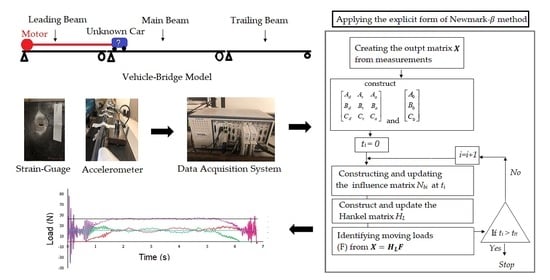
Funding

This research was funded by Australian Research Council under the discovery program grant number DP160103197.

Institutional Review Board Statement

Not Applicable.

Informed Consent Statement

Not Applicable.

Data Availability Statement

Data is contained within the article.

Conflicts of Interest

The authors declare no conflict of interest.

References

  1. Chen, S.; Xia, H.; Zhang, J. Review on bridge structural damage identification techniques based on bridge-vehicle coupled vibration analysis. China Saf. Sci. J. 2007, 17, 148–155. [Google Scholar]
  2. Law, S.-S.; Zhu, X.-Q. Damage Models and Algorithms for Assessment of Structures under Operating Conditions; CRC Press, Taylor & Francis Group: London, UK, 2009. [Google Scholar]
  3. Siringoringo, D.M.; Fujino, Y. Estimating Bridge Fundamental Frequency from Vibration Response of Instrumented Passing Vehicle: Analytical and Experimental Study. Adv. Struct. Eng. 2012, 15, 417–433. [Google Scholar] [CrossRef]
  4. Hester, D.; Gonzalez, A. A wavelet-based damage detection algorithm based on bridge acceleration response to a vehicle. Mech. Syst. Signal Process. 2012, 28, 145–166. [Google Scholar] [CrossRef] [Green Version]
  5. Sun, Z.; Zhang, Y.; Tong, S. Review of Bridge Damage Detection Based on Coupled Vehicle-Bridge Vibration. China Saf. Sci. J. 2013, 29, 1–8. [Google Scholar]
  6. González, A.; Hester, D. An investigation into the acceleration response of a damaged beam-type structure to a moving force. J. Sound Vib. 2013, 332, 3201–3217. [Google Scholar] [CrossRef] [Green Version]
  7. Malekjafarian, A.; McGetrick, P.J.; Obrien, E.J. A Review of Indirect Bridge Monitoring Using Passing Vehicles. Shock. Vib. 2015, 2015, 1–16. [Google Scholar] [CrossRef] [Green Version]
  8. Zhu, X.Q.; Law, S.S. Structural Health Monitoring Based on Vehicle-Bridge Interaction: Accomplishments and Challenges. Adv. Struct. Eng. 2015, 18, 1999–2015. [Google Scholar] [CrossRef]
  9. Zhu, X.; Cao, M.; Ostachowicz, W.; Xu, W. Damage Identification in Bridges by Processing Dynamic Responses to Moving Loads: Features and Evaluation. Sensors 2019, 19, 463. [Google Scholar] [CrossRef] [Green Version]
  10. Rashidi, M.; Mohammadi, M.; Kivi, S.S.; Abdolvand, M.M.; Truong-Hong, L.; Samali, B. A Decade of Modern Bridge Monitoring Using Terrestrial Laser Scanning: Review and Future Directions. Remote Sens. 2020, 12, 3796. [Google Scholar] [CrossRef]
  11. Gonzalez, A.; Dowling, J.; O’Brien, E.J.; Žnidarič, A. Testing of a Bridge Weigh-in-Motion Algorithm Utilising Multiple Longitudinal Sensor Locations. J. Test. Eval. 2012, 40, 961–974. [Google Scholar] [CrossRef]
  12. Ojio, T.; Carey, C.H.; Obrien, E.J.; Doherty, C.; Taylor, S.E. Contactless Bridge Weigh-in-Motion. J. Bridge Eng. 2015, 21, 04016032. [Google Scholar] [CrossRef] [Green Version]
  13. Wang, H.; Nagayama, T.; Zhao, B.; Su, D. Identification of moving vehicle parameters using bridge responses and estimated bridge pavement roughness. Eng. Struct. 2017, 153, 57–70. [Google Scholar] [CrossRef]
  14. Yu, Y.; Cai, C.S.; Deng, L. State-of-the-art review on bridge weigh-in-motion technology. Adv. Struct. Eng. 2016, 19, 1514–1530. [Google Scholar] [CrossRef]
  15. Chan, T.; Yu, L.; Law, S. Comparative Studies on Moving Force Identification from Bridge Strains in Laboratory. J. Sound Vib. 2000, 235, 87–104. [Google Scholar] [CrossRef]
  16. Law, S.; Zhu, X. Study on Different Beam Models in Moving Force Identification. J. Sound Vib. 2000, 234, 661–679. [Google Scholar] [CrossRef]
  17. Law, S.; Fang, Y. Moving Force Identification: Optimal State Estimation Approach. J. Sound Vib. 2001, 239, 233–254. [Google Scholar] [CrossRef]
  18. Zhu, X.; Law, S. Orthogonal Function in Moving Loads Identification on a Multi-Span Bridge. J. Sound Vib. 2001, 245, 329–345. [Google Scholar] [CrossRef]
  19. Zhu, X.; Law, S.S. Moving Loads Identification Through Regularization. J. Eng. Mech. 2002, 128, 989–1000. [Google Scholar] [CrossRef]
  20. Zhu, X.; Law, S. Moving load identification on multi-span continuous bridges with elastic bearings. Mech. Syst. Signal Process. 2006, 20, 1759–1782. [Google Scholar] [CrossRef]
  21. Asnachinda, P.; Pinkaew, T.; Laman, J. Multiple vehicle axle load identification from continuous bridge bending moment response. Eng. Struct. 2008, 30, 2800–2817. [Google Scholar] [CrossRef]
  22. Oliva, J.; Goicolea, J.M.; Antolín, P.; Astiz, M.Á. Relevance of a complete road surface description in vehicle-bridge interaction dynamics. Eng. Struct. 2013, 56, 466–476. [Google Scholar] [CrossRef]
  23. Zhou, Y.; Zhou, S.; Deng, L.; Chen, S.; Yi, W. Research on moving load identification based on measured acceleration and strain signals. Int. J. Lifecycle Perform. Eng. 2019, 3. [Google Scholar] [CrossRef]
  24. Wu, S.Q.; Law, S.S. Statistical moving load identification including uncertainty. Probabilistic Eng. Mech. 2012, 29, 70–78. [Google Scholar] [CrossRef]
  25. Eshkevari, S.S.; Matarazzo, T.J.; Pakzad, S.N. Simplified vehicle–bridge interaction for medium to long-span bridges subject to random traffic load. J. Civ. Struct. Health Monit. 2020, 10, 693–707. [Google Scholar] [CrossRef]
  26. Liu, K.; Law, S.S.; Zhu, X.Q.; Xia, Y. Explicit form of an implicit method for inverse force identification. J. Sound Vib. 2014, 333, 730–744. [Google Scholar] [CrossRef]
  27. Wang, T.; Wan, Z.; Wang, X.; Hu, Y. A novel state space method for force identification based on the Galerkin weak formulation. Comput. Struct. 2015, 157, 132–141. [Google Scholar] [CrossRef]
  28. Agostinacchio, M.; Ciampa, D.; Olita, S. The vibrations induced by surface irregularities in road pavements—A Matlab® approach. Eur. Transp. Res. Rev. 2014, 6, 267–275. [Google Scholar] [CrossRef] [Green Version]
  29. Ferdek, U.; Łuczko, J. Vibration analysis of a half-car model with semi-active damping. J. Theor. Appl. Mech. 2016, 54, 321. [Google Scholar] [CrossRef] [Green Version]
  30. Setiawan, J.D.; Safarudin, M.; Singh, A. Modeling, simulation and validation of 14 DOF full vehicle model. In Proceedings of the International Conference on Instrumentation, Communication, Information Technology, and Biomedical Engineering 2009, Bandung, Indonesia, 23–25 November 2009; Institute of Electrical and Electronics Engineers (IEEE): Piscataway, NJ, USA, 2009; pp. 1–6. [Google Scholar]
  31. Rajamani, R. Vehicle Dynamics and Control; Springer: Berlin/Heidelberg, Germany, 2011. [Google Scholar]
  32. Kurczyk, S.; Pawełczyk, M. Fuzzy Control for Semi-Active Vehicle Suspension. J. Low Freq. Noise Vib. Act. Control. 2013, 32, 217–225. [Google Scholar] [CrossRef] [Green Version]
  33. Yang, Y.-B.; Lin, B.-H. Vehicle-Bridge Interaction Analysis by Dynamic Condensation Method. J. Struct. Eng. 1995, 121, 1636–1643. [Google Scholar] [CrossRef]
  34. Law, S.S.; Bu, J.Q.; Zhu, X.Q.; Chan, S. Vehicle axle loads identification using finite element method. Eng. Struct. 2004, 26, 1143–1153. [Google Scholar] [CrossRef]
  35. Feng, D.; Sun, H.; Feng, M.Q. Simultaneous identification of bridge structural parameters and vehicle loads. Comput. Struct. 2015, 157, 76–88. [Google Scholar] [CrossRef]
  36. Aster, R.C.; Borchers, B.; Thurber, C.H. Parameter Estimation and Inverse Problems; Academic Press: Cambridge, MA, USA, 2004. [Google Scholar]
  37. Golub, G.H.; Heath, M.; Wahba, G. Generalized Cross-Validation as a Method for Choosing a Good Ridge Parameter. Technometrics 1979, 21, 215–223. [Google Scholar] [CrossRef]
  38. Hancen, P.C. Regularization Tools, a Matlab Package for Analysis and Solution of Discrete Ill-Posed Problems; Springer: Berlin/Heidelberg, Germany, 2008. [Google Scholar]
  39. Mulcahy, N.L. Bridge response with tractor-trailer vehicle loading. Earthq. Eng. Struct. Dyn. 1983, 11, 649–665. [Google Scholar] [CrossRef]
Figure 1. Vehicle-bridge interaction system.
Remotesensing 13 02291 g001
Figure 2. An element under moving load.
Remotesensing 13 02291 g002
Figure 3. Calculating the vehicle/bridge responses and the true moving loads by the explicit form of Newmark-β method.
Remotesensing 13 02291 g003
Figure 4. Moving load identification by the explicit form of Newmark-β method.
Remotesensing 13 02291 g004
Figure 6. Identified loads at road roughness level C at a of speed 10 m/s and with 2% noise: (a) rear axle load identification, (b) front axle load identification.
Remotesensing 13 02291 g006
Figure 7. Three-span bridge model.
Remotesensing 13 02291 g007
Figure 8. Effect of noise on load identification at road roughness level A and speed of 40 m/s: (a) rear axle load identification, (b) front axle load identification.
Remotesensing 13 02291 g008
Figure 9. Identified loads at road roughness level B, speed 15 m/s and 0% noise: (a) rear axle load identification, (b) front axle load identification.
Remotesensing 13 02291 g009
Figure 10. Identified loads at road roughness level B, speed 15 m/s and 2% noise: (a) rear axle load identification, (b) front axle load identification.
Remotesensing 13 02291 g010
Figure 11. Experimental set-up of the vehicle-bridge system.
Remotesensing 13 02291 g011
Figure 12. (a) Details at the left-hand support of the main beam, (b) the two-axle model vehicle.
Remotesensing 13 02291 g012
Figure 13. (a) Data acquisition system, (b) strain gauge and (c) accelerometer.
Remotesensing 13 02291 g013
Figure 14. Impact hammer.
Remotesensing 13 02291 g014
Figure 15. Hammer impact force.
Remotesensing 13 02291 g015
Figure 16. Acceleration response at location 3L/16.
Remotesensing 13 02291 g016
Figure 17. FFT of acceleration responses at locations L/2 and 3L/16.
Remotesensing 13 02291 g017
Figure 18. The effect of N f on the error of the reconstructed strain.
Remotesensing 13 02291 g018
Figure 19. Measured and reconstructed strain at mid-span.
Remotesensing 13 02291 g019
Figure 20. Comparison of the effects of a small Nf and the optimized value on the identified axle loads. (a) Identified front axle load, (b) identified rear axle load.
Remotesensing 13 02291 g020
Figure 21. Identified front, rear, and resultant load in comparison with the static axle load and static weight of the car (sensor placement #2).
Remotesensing 13 02291 g021
Figure 22. The effect of sampling frequency on the identified loads at speed 0.47 m/s. (a) front axle load, (b) rear axle load, (c) resultant axle load.
Remotesensing 13 02291 g022
Figure 23. Identified front, rear, and resultant load in comparison with the static axle load and static weight of the vehicle (speed: 0.75 m/s).
Remotesensing 13 02291 g023
Figure 5. Identified loads at road roughness level A with speed 15 m/s using sensor placement S7. (a) Rear axle load identification, (b) Front axle load identification.
Remotesensing 13 02291 g005
Table 1. Vehicle parameters.
mv = 17735 kgmt1 = 1500 kgMt2 = 1000 kg
Iv = 1.47E5 Nm2Ks1 = 2.47E6 N/mKs2 = 4.23E6 N/m
a1 = 0.519 mKt1 = 1.75E6 N/mKt2 = 3.5E6 N/m
a2 = 0.481 mCs1 = 3E4 N/m/sCs2 = 4E4 N/m/s
S = 4.27 mCt1 = 3.9E3 N/m/sCt2 = 4.3E3 N/m/s
Table 2. Bridge parameters.
L = 30 mEI = 2.5 × 10¹⁰ Nm2ρA = 5 × 10³ kg/mDamping ratio for all modes = 0.02
Table 3. Sensor Placement.
Sensor CaseSensor No.Sensor Location
S331/3L, 2/3L,4/5L
S441/8L, 1/4L, 1/2L, 3/4L
S551/8L, 1/4L, 1/2L, 3/4L, 7/8L
S661/8L, 1/4L, 1/2L, 5/8L, 3/4L, 7/8L
S771/8L, 1/4L, 3/8L, 1/2L, 5/8L, 3/4L, 7/8L
Table 5. The relative error (%) of moving load identification from sensor placement S7.
Speed (m/s)10203040
Road roughnessABCABCABCABC
Front axle load1.19.512.22.28.1-1.88.5-1.28.9-
Rear axle load1.56.519.62.89.6-2.214.3-2.48.6-
Table 6. Percentage errors of the identified moving loads at different levels of speed and noise.
Speed (m/s)15203040
Measurement noise (%)025025025025
Front axle load0.013.23.40.012.84.80.012.63.10.022.93.6
Rear axle load0.163.53.60.23.65.90.34.63.80.463.84.1
Table 7. The relative error (%) of the identified forces at noise 0%.
Speed (m/s)15203040
Road roughnessABCABCABCABC
Front axle load0.010.050.250.010.01-0.10.1-0.02--
Rear axle load0.160.150.130.20.21-0.40.3-0.46--
Table 8. The relative error (%) of the identified forces at 2% noise.
Speed (m/s)15203040
Road roughnessABCABCABCABC
Front axle load3.210.832.52.812.7-2.69.6-2.3--
Rear axle load3.511.829.23.618.0-4.612.4-3.4--
Table 9. Calculated and measured natural frequencies of the test beam (Hz).
Modal Frequency1st2nd3rd
Measured6.272761.17
Calculated6.4825.7857.38
Error 3.34%4.52%6.19%
Table 10. Sensor arrangements.
Case NumberNumber of SensorsSensor Location
L/8L/43L/8L/25L/86L/87L/8
#17*******
#23 * * *
#33* * *
#43 ***
#53* * *
#64****
#74* ** *
#84** **
#94* * * *
#105** * **
#115* *** *
#125 *****
#136*** ***
#141 *
#152 * *
#162 * *
#172* *
*. The location with sensor
Table 11. The percentage error for different sensor arrangements.
Case NumberNumber of SensorsThe Percentage Error (%)
Strain at Mid-SpanAverage of Identified Front Axle LoadAverage of Identified Rear Axle LoadAverage of Resultant Identified Load
#171.750.090.250.08
#232.971.032.460.72
#334.792.333.532.93
#434.061.660.350.66
#532.553.773.870.05
#644.964.103.80.51
#742.004.154.380.12
#843.760.031.020.49
#942.310.512.561.03
#1052.510.531.160.32
#1151.860.282.120.92
#1251.990.321.550.61
#1361.800.360.660.15
#14110.780.310.650.48
#1525.281.700.040.87
#16211.021.740.180.96
#1729.078.8211.871.52
Table 12. The percentage error at different levels of sampling frequency at speed 0.47 m/s.
Sampling Frequency (Hz)100200300600
Reconstructed strain error (%)3.352.972.52.28
Table 13. The percentage error at different levels of speed.
Speed (m/s)0.470.750.97
Reconstructed strain error (%)2.972.833.62
Table 4. The relative error (%) of the identified forces for different sensor placements.
Sensor CaseNoise Level (%)Front Axle LoadRear Axle Load
S3000.25
22.682.8
54.193.71
S4000.23
22.32.73
53.113.18
S500.222.9
23.034.12
53.24.03
S600.312.42
22.782.92
52.63.29
S7000.24
22.152.01
53.33.85
Publisher’s Note: MDPI stays neutral with regard to jurisdictional claims in published maps and institutional affiliations.

