
Analysis of Salt Lake Volume Dynamics Using Sentinel-1 Based SBAS Measurements: A Case Study of Lake Tuz, Turkey


1
Department of Geomatics Engineering, Faculty of Engineering and Natural Sciences, Gumushane University, Gumushane 29000, Turkey
2
Building of Graduate School, Ayazaga Campus, Istanbul Technical University, Istanbul 34469, Turkey
3
Department of Geomatics Engineering, Civil Engineering Faculty, Istanbul Technical University, Istanbul 34469, Turkey
*
Author to whom correspondence should be addressed.
Remote Sens. 2021, 13(14), 2701; https://doi.org/10.3390/rs13142701
Submission received: 24 May 2021
/
Revised: 3 July 2021
/
Accepted: 5 July 2021
/
Published: 9 July 2021
(This article belongs to the Special Issue Remote Sensing for Wetland Inventory, Mapping and Change Analysis)
Abstract
:As one of the largest hypersaline lakes, Lake Tuz, located in the middle of Turkey, is a key waterbird habitat and is classified as a Special Environmental Protection Area in the country. It is a dynamic lake, highly affected by evaporation due to its wide expanse and shallowness (water depth <40 cm), in addition to being externally exploited by salt companies. Monitoring the dynamics of its changes in volume, which cause ecological problems, is required to protect its saline lake functions. In this context, a spatially homogeneous distributed gauge could be critical for monitoring and rapid response; however, the number of gauge stations and their vicinity is insufficient for the entire lake. The present study focuses on assessing the feasibility of a time-series interferometric technique, namely the small baseline subset (SBAS), for monitoring volume dynamics, based on freely available Sentinel-1 data. A levelling observation was also performed to quantify the accuracy of the SBAS results. Regression analysis between water levels, which is one of the most important volume dynamics, derived by SBAS and levelling in February, April, July and October was 67%, 80%, 84%, and 95% respectively, for correlation in the range of 10–40 cm in water level, and was in line with levelling. Salt lake components such as water, vegetation, moist soil, dry soil, and salt, were also classified with Sentinel-2 multispectral images over time to understand the reliability of the SBAS measurements based on interferometric coherence over different surface types. The findings indicate that the SBAS method with Sentinel-1 is a good alternative for measuring lake volume dynamics, including the monitoring of water level and salt movement, especially for the dry season. Even though the number of coherent, measurable, samples (excluding water) decrease during the wet season, there are always sufficient coherent samples (>0.45) over the lake.
1. Introduction
In providing a productive ecosystem and suitable habitat for a wide variety of plant and animal species, wetlands are vital ecological and important social-economic areas [1,2]. It is important to protect and monitor wetlands, which feed groundwater resources, increase the agricultural soil fertility, regulate the water cycle, and reduce carbon emissions, among other functions [3,4]. Policies aiming at the management of wetlands strive to monitor their physical, chemical, and biological characteristics by measuring variations in water level/area/volume, pollutant factors, input–output, and the impact of the surrounding industries on the lake [5]. Among these variations, volume dynamics is an important parameter that directly affects the population of plant and animal communities in this habitat; climate change and human activities are the main drivers of this change [6,7,8]. In this context, information on deformation in the lake surface and its water levels, with a high temporal and spatial resolution (frequency of gauge stations), plays an important role in wetland monitoring [9]. However, many lakes do not have gauge stations or they are not sufficient in frequency and number to extract hydrological information for the entire lake [10]. In addition to the low spatial resolution of these stations, there may be difficulties in acquiring data from institutions and organizations that manage and trade the data gathered by gauge stations [11]. In this regard, remote sensing (RS) instruments developed in parallel with technological advances are an ideal platform for solving such current problems and are highly utilized in assessing the volume dynamics of wetlands [12].
Since the United States Geological Survey (USGS) began to provide data freely to all users following a data policy change in 2008, it was easier for researchers to access RS (new and archived Landsat) data [13]. Additionally, the European Commission’s Copernicus program, which launched its first satellite in 2014, started to offer alternatives free of charge for users. This program, created by the European Space Agency (ESA), is the European Union’s Earth Observation (EO) program, which aims to monitor our planet and its environment. It provides freely available information services to its users via satellites and in situ data such as ground stations, airborne sensors, and seaborne sensors. Since the launch of the Sentinel-1A SAR satellite in 2014, EO data have been actively used in many research areas, such as agriculture, climate change, the environment, marine observation, insurance, disaster management, and the blue economy [14]. Sentinel-1 SAR images with a high spatial resolution (5 m × 20 m on the ground) provide dual-polarization (VV and VH) backscatter coefficients in the C-band. Their high temporal resolution (12- and 6-day repeat cycle option) and their day, night, and all-weather imaging capability have excellent application prospects in the field of environmental monitoring [15,16]. The short revisit time is especially advantageous for observing dynamic areas with rapid changes, such as wetlands, landslide zones, and sinkhole areas [17,18,19,20].
With the launch of the Sentinel-2A in 2015, Copernicus made both SAR and optical satellite images available free of charge. The purpose of the Sentinel-2 mission is to create an operational multispectral EO system that ensures sustainability and works in harmony with the Landsat and Spot satellites [21]. Sentinel-2 has some advantages over Landsat. It has higher spatial resolution and higher spectral resolution in the near-infrared region and also has three vegetation red-edge bands. The Sentinel-2 sensor, the EO satellite of the Copernicus program, has 12 bands with spatial resolutions of 10 m (four visible and near-infrared bands), 20 m (six red-edge and shortwave infrared bands), and 60 m (three atmospheric correction bands) [22,23,24]. It is also important, especially for long-term monitoring, that the Sentinel missions are guaranteed to continue until 2030 [25].
In this context, the high temporal resolution, coupled with free availability, achieved by optical Sentinel-2 and SAR Sentinel-1 images paves the way for new hydrological applications aimed at the identification and monitoring of wetlands [26,27].
The Single Look Complex (SLC) imaging mode of Sentinel-1, with high temporal resolution across large areas, makes it possible to use large stacks of interferometric SAR (InSAR) data to monitor surface displacements on the Earth’s surface over time [28]. In this context, many different studies have been conducted on interferometric Sentinel-1 data coupled with the persistent scatter interferometry (PSInSAR) method [29], specifically in urban monitoring, such as in reclamation areas [30], dams [31], bridges [32], and buildings [33]. The popularity of the PSInSAR technique lies in the fact that it obviates the need for time-consuming and costly geodetic surveying methods, and provides detailed information about surface displacement. However, when it comes to surfaces in rural settings, as opposed to urban ones, PSInSAR implementation is challenging due to the lack of persistent scatters in high coherence targets [34]. In this context, another powerful time-series InSAR method, namely small baseline subsets (SBAS), offers not only unique surface change (deformation) information but also information related to the dielectric constant and structure of the surface [35]. When determining the main and dependent pairs for interferograms in the SBAS network, they are selected according to the average baseline parameters for the signal of interest, without considering the temporal baseline [36]. The SBAS technique provides highly sensitive information about surface deformations in urban centers and open areas for determining land subsidence [37,38]. However, in highly complex situations, such as monitoring water level changes and salt movement, ignoring the temporal separation of interferograms results in poor coherence. In wetlands, INSAR measurements and water level determinations are related to the characteristics of the region [39]. Nevertheless, there are distinct seasonal deformation features in areas close to the water body [40]. For this reason, the temporal baseline should be as small as possible in the determination of volume dynamics, such as cases in which the water level of wetlands is being monitored [41].
In this study, we aimed to monitor the volume dynamics, including water level and salt movement, in one of the largest hypersaline lakes in the world [42], namely Lake Tuz (Turkey), using EO satellites of the Copernicus program. For this purpose, the SBAS method, an advanced interferometric technique, was applied to Sentinel-1 SAR data from November 2017 to January 2019. We have compared the levelling measurements conducted in the field with those calculated using SBAS in terms of water level accuracy. Additionally, the consistency and applicability of the SBAS methodology have been evaluated with meteorological and optical Sentinel-2 data to understand whether SBAS meets the requirements of water level information in the salt lake area, where there is a dynamic transition among the salt lake components, namely water, vegetation, salt, moist soil, and dry soil.
2. Materials and Methods
2.1. Study Region
Lake Tuz, located in the middle of Turkey, is one of the largest hypersaline lakes in the world and the second-largest lake in Turkey. It is mainly fed by underground water. With specific kinds of flora and fauna, it was declared a Special Environmental Protection Area (SEPA) by Turkey’s Cabinet of Ministers in 2000. This type of lake is generally shallow and saline, with its salinity being about 35%. Lake Tuz covers an area approximately 1500 km2, with a length of 80 km and a width of 50 km (Figure 1). Its bright visibility from space, strong reflection, and flatness make it one of the EO’s eight calibration sites in the world. The lake is categorized as a wetland, and its salinity varies seasonally with the water level, being at its lowest in the wet season and highest in the dry season, due to evaporation [43,44]. In the winter, it spreads over a large area due to the effect of precipitation and dissolves the salt particles, while, in the summer approximately 95% of the lake dries up and turns into a salt flatland [45,46]. More than half of Turkey’s salt needs are covered by salt pans in the lake [47]. It is known that approximately 1200 km² of the Lake Tuz area is a salt region. The lake’s salt reservoir totals approximately 210 million tons. With this reserve potential, the lake is the second-largest source of salt production in the world [48]. The water level, and hence the salt pans, are particularly influenced by industrial activities, as salt lakes are the main areas where the salt industry operates.
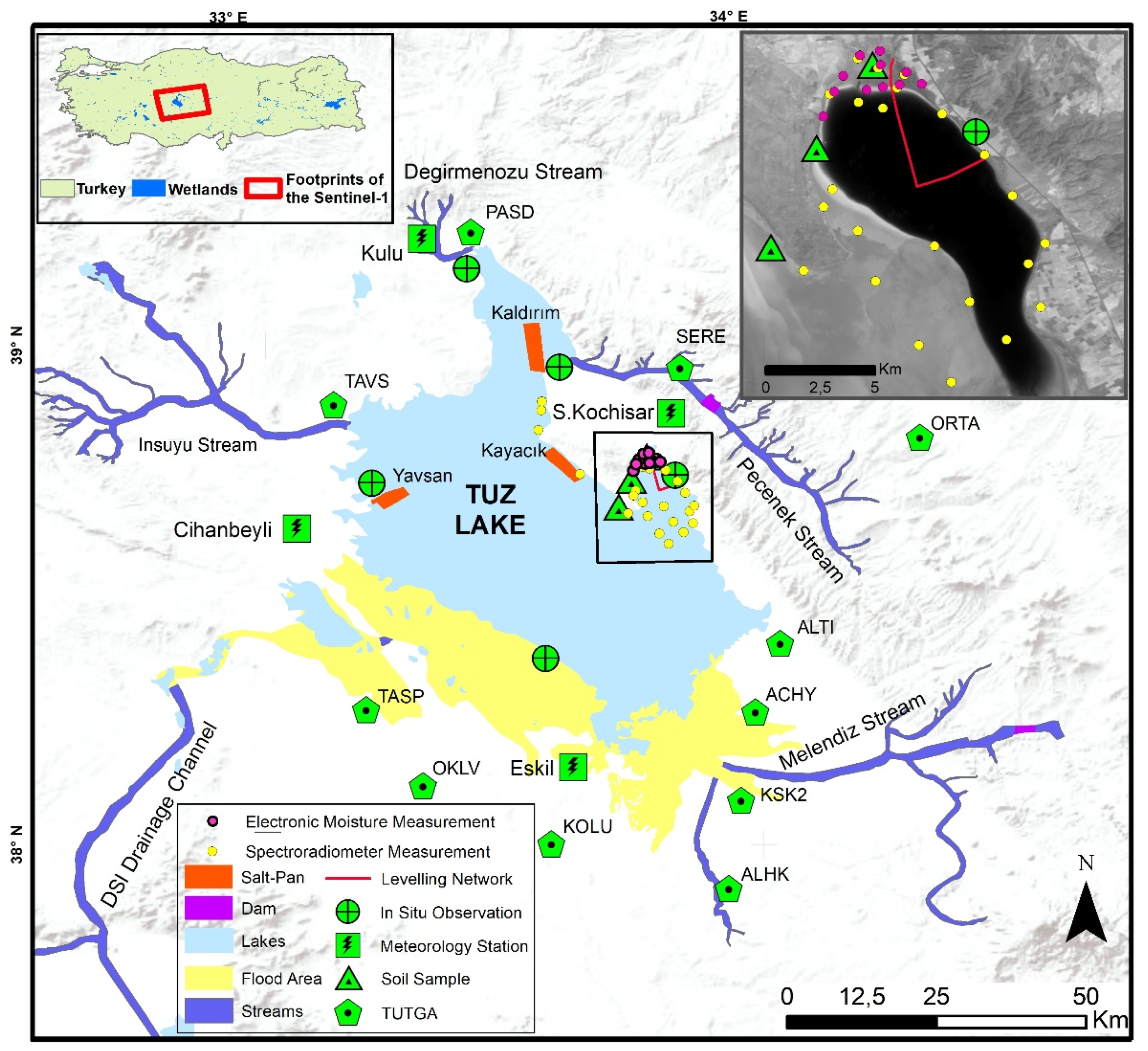
In the lake, industrial salt production starts around mid-April by drawing water from the lake to the salt pan. This continues for four or five months depending on weather conditions, as high temperatures are required for evaporation. Salt formation starts in August and continues until October. In October, underground waters emerge from numerous crevices to feed the lake bed and thus the salt production cycle continues. There are four meteorological stations and two dams around Lake Tuz, as shown in Figure 1. The dams were built on the Melendiz and Pecenek streams, which feed the lake. Moreover, the beds of the Degirmenozu and Insuyu streams were modified to feed other lakes that were about to dry out. It is worth noting that the channel of the General Directorate of State Hydraulic Works (DSI), located in the southwest region where seasonal floods occur every year, is the only source that directly feeds Lake Tuz. The lake system is well represented on the eastern side, where detailed field work (electronic moisture measurement, spectroradiometer measurement, and levelling measurement) was carried out. Eleven points of the Turkish National Fundamental GPS Network (TUTGA) are homogeneously distributed in the study area, and GPS measurements taken from the salt pans in the Lake Tuz are used as calibration data for SBAS results in the interferogram calibration stage; these data were obtained from the General Directorate of Mapping (HGM).
2.2. Methodology
Figure 2 depicts the general framework of the methodology used in this work, which is based on Sentinel-1/-2 and field survey data. An interferometric stack of Sentinel-1 data acquired over Lake Tuz was used first to obtain information on the volume dynamics by the SBAS method using ENVI SARscape software [49,50]. Sentinel-2 and field survey data (GPS, temperature, moisture, and levelling measurements) were used subsequently to evaluate the feasibility of the method for Lake Tuz in terms of the temporal dynamics among its components: water, vegetation, salt, moist soil, and dry soil.
In the study, Sentinel-1 and Sentinel-2 satellite data obtained freely from the EO Copernicus program were used. Short revisit time, which is an important feature in monitoring areas with rapid changes, was available in both the SAR and optical satellite data (Table 1). The Copernicus Open Access Hub has provided Level-2A products of Sentinel-2 imagery data over Europe from 28 March 2017 [51]. Sentinel-2 Multispectral Instrument Level 2A (S2-MSIL2A) imagery was used; this delivered atmospherically and geometrically corrected bottom-of-atmosphere (BOA) reflectance images.
The Sentinel-1 Interferometric Wide (IW) swath mode with C-band (radar frequency of 5.4 GHz) SAR sensors were considered for applying the SBAS method and determining the water level. Thirty-four ascending VV polarized Sentinel-1 (orbit no 87) images were used, covering the period from 30 November 2017 to 12 January 2019. VV polarization was preferred out of the two polarization options because it produces better results in wetlands [52]. Since the use of ascending and descending tracks in flat basins such as Lake Tuz gave consistently similar results, a single track was preferred in this study [53].
The SBAS technique is a DInSAR approach that uses a large number of SAR acquisitions, based the increase in the quantity of existing data sets and the developments in interferometric processes, thus minimizing the potential for negative data features such as decorrelation, atmospheric propagation delay, and topographic errors. SBAS uses singular value decomposition (SVD) to connect independent interferograms in time, correcting for atmospheric and topographic effects. TUTGA points in the region and salt pans in the lake were used as distributed scatterer (DS) candidates. These DS candidates add an advantage to the study area compared to other lakes. Interferogram pairs were generated with a 0.45 coherence parameter threshold and then removed to the topographic phase using the shuttle radar topographic mission (SRTM) height as the topographic reference data, then the Wavelet functionality atmospheric correction was applied. The interferogram stack was unwrapped and the slant range was defined as multi-look. Ground control points were selected to refine the orbits and remove possible phase ramps from the unwrapped phase stack. Temporal coherence, calculated on the random motion of scatterers within a resolution cell, was considered as one univariate exponential function of time. It ranged from 0 (without reliable information) to 1 (reliable information without noise). A threshold was used to ensure that the selected SAR pixels give reliable and consistent results. Therefore, reliable SAR pixels were selected by setting a threshold value of 0.45 to remove unreliable pixels from the SBAS results derived from the Sentinel-1 data [54,55]. The SBAS inversion kernel was then applied to determine the initial displacement results and the residual topography. In the second inversion stage, the SBAS inversion kernel was applied to generate the displacement time series. By applying the geometric correction, the results were transformed on the earth coordinate system (see Figure 2).
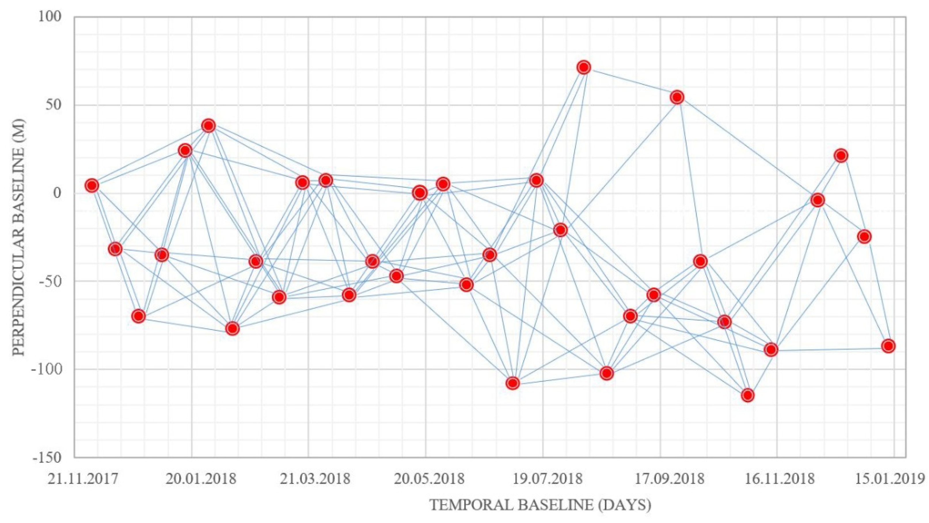
In order to reduce the temporal decorrelation and increase the number of coherent samples, SAR images were selected according to their spatial and temporal baselines. As a result, a total number of 128 interferograms were generated, and time series was produced from all images in the stated period, using a perpendicular baseline below 100 meters and temporal baseline below 60 days (Figure 3).
To analyze the potential of the SBAS methodology for water level monitoring in the Lake Tuz environment, Sentinel-2 images were used to understand the dynamics of the salt lake components and their impact on the SBAS measurements. Four Sentinel-2 images with 10 m and 20 m resolutions were selected to represent seasonal variations: 2 February, 17 April, 10 August and 29 October, 2018. The water withdrawal periods and salt harvesting were also taken into consideration.
2.3. Field Surveys
As shown in highlighted part of Figure 1, field work was conducted in the northeast region of Lake Tuz, which has reflective features characteristic of the entire lake [56,57,58]. The field surveys were carried out in October, when the region was in the driest season; February, when the region was at its wettest; and in the transition months between these two seasons: April and July. Thus, optimum reference data were obtained by performing measurements with levelling and GPS for comparison with the SBAS results when the water was at a minimum and maximum level.
Spectroradiometer measurements were carried out to better classify the satellite images and to provide the correlations between the ground and satellite data simultaneously with the satellite pass time on 17 April 2018, when information on all the salt lake components could be obtained. The spectra of the salt lake components were obtained by a handheld spectroradiometer, an Analytical Spectral Device (ASDInc., Boulder CO, USA) with a spectral range of 325–1075 nm, which were used as ground-truth reference spectra for temporal Sentinel-2 image classification. Reflectance calibration was done with white reference material, and spectral measurements were conducted at 15 sample points for each class, enabling the extraction of the average radiance of the components for the wavelength in the range of 325–1075 nm. At each sample point, the temperature and moisture of the soil was also recorded with a KCB-300 Portable Soil Survey Instrument and a moisture PH meter. Figure 4 shows the mean spectral reflectance curve and the wavelength ranges corresponding to the Sentinel-2 bands. The graph shows Sentinel-2 bands (excluding SWIR bands) with 10 m and 20 m spatial resolution covering the wavelength range of the spectroradiometer.
The precise geometric levelling technique was performed in four field surveys to investigate the potential of the SBAS method used in determining the lake volume dynamics. The geometric levelling sought to obtain control data with mm precision. The loop is a line measuring approximately 15 km, 8.8 km of which is inside Lake Tuz and 6.2 km outside. While these surveys were being made, 2 measurements with 2 different rods were made in same each point with only one topographer and the average was taken. In the measurements made in this lake, where the slope is very low, there was very little difference between the 2-point measurements that were averaged. Geometric levelling measurement results, consisting of north-south and east-west directions, were obtained for a total of 250 points were recorded among 356 benchmarks. Thanks to GPS/Leveling measurements, the positions of each rod measurements were recorded. Measurements were made from the same places in subsequent field surveys. In addition, safeguarded and stable benchmarks were taken as reference outside the lake. As a result of this technique, the network was closed with a 2 cm error limit below the tolerance limit of 5.8 cm. Figure 5 shows two images taken from the area close to the shore of the lake. In addition, it was seen that it would be more appropriate and faster to take geometric leveling measurements with a barcoded invar rod. The water-covered area in the image on the left turned into a salt-covered area in the dry period due to evaporation, as can be seen in the image on the right.
3. Results
3.1. Analysis of Sentinel-1 SBAS Measurement
The LOS direction velocity map, derived from 128 interferograms with SBAS, is shown in Figure 6a. Pixels having a coherence value less than 0.45 are masked out in the final displacement map, which mainly sows water and moist saline lands. Velocities in the positive direction are shown in green with a maximum of 2.75 cm/year, while velocities in the negative direction are shown in red with a minimum of −2.75 cm/year. Significant surface variation was evident around Lake Tuz, especially in the middle of the lake and where the salt pans are located. Although there were a limited number of samples from the inner part of the lake, there were enough to see surface variation trends due to salt-related activities.
In general, one of the most difficult challenges of InSAR in wetland monitoring is decorrelation, due to the complex interaction of microwaves, the morphology of the canopy and the water. However, in the context of salt lakes, the high salt content of the water makes interferometry measurements more stable. The photographs taken in the field in Figure 6c show the main surface characteristics of the lake. The first surface, shown in photograph P1, had the highest volume of salt density suspended in water, which led to the limited information from the area. At the P2 point, it is seen that salt masses are collected and much information was obtained, as can be clearly seen in the area with a water height of about 10 cm. The dry soil and pure salt surfaces represented by photographs P3 and P4 respectively, were characterized by high SBAS measurements due to the high amount of stable information. Figure 6b shows the spatial distribution of the standard deviations of the SBAS measurements. While the standard deviation is high in the lake, which has a dynamic structure, the salt pans in the lake are the opposite, and have high reflectivity. Although the maximum standard deviation of the measurement reached 4.88 cm/year, 60% of the measurements had a standard deviation less than 1 cm/year, highlighting the reliability of the measurements.
3.2. The Influence of Temporal Variations of the Salt Lake Components on the SBAS Results
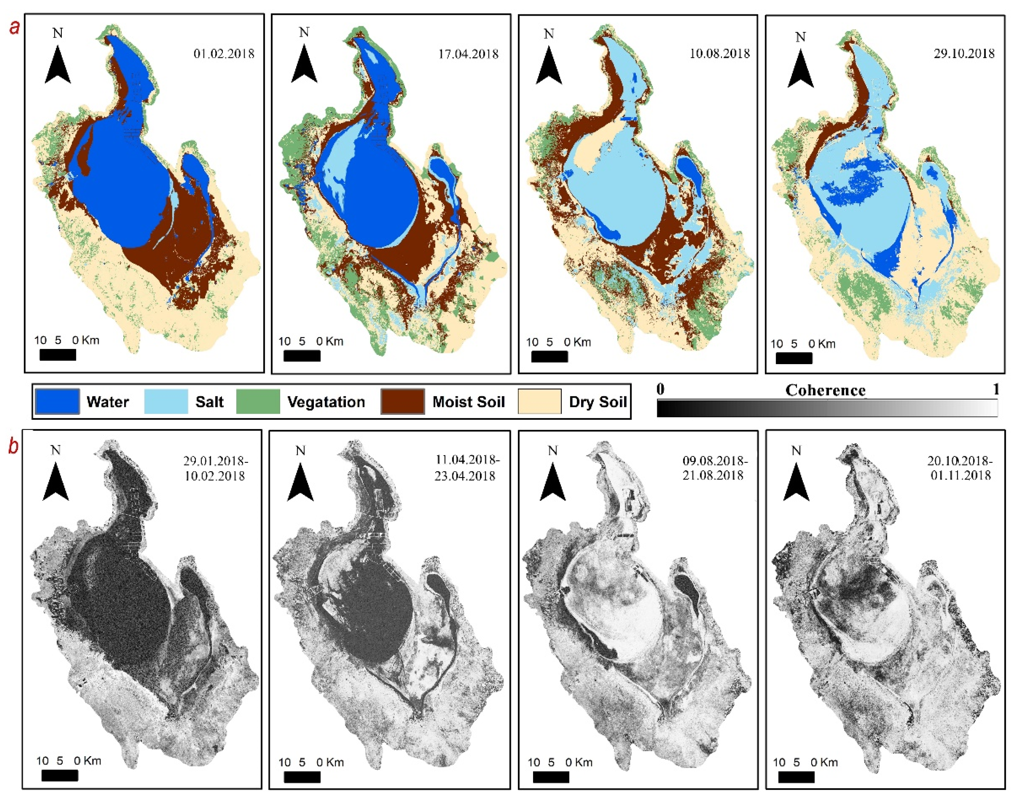
To understand the seasonal transition and influence of the salt industry on the salt lake components (water, salt, vegetation, moist soil, and dry soil), Sentinel-2 images were classified with a Support Vector Machine (SVM) classifier. The SVM classifier was chosen due to its simplicity and high performance with few samples in the wetland environment [59,60,61]. In the classification process with the SVM, the radial basis function kernel was preferred, and optimum parameter values were determined by the cross-validation method. In the field surveys carried out in different parts of the lake, class information about the region was collected by hand GPS and spectroradiometer; half of this was used as training data at the classification stage the other half was used as ground truth data. The classification performance of the SVM models obtained was calculated using the test data sets. According to the 100 ground truth data, the overall accuracy of the SVM classifier was 88.7%, 87.9%, 86.2%, and 87.5% for the February, April, August, and October images, respectively. Figure 7 shows the SVM classification results and the corresponding coherence images derived from the closest possible interferogram pairs. It was observed that August was almost completely dry with no rainfall (see Figure 7). This month saw the lowest occurrence of water at the site. It continued like that until October, when Lake Tuz started to be refilled with water. In February, water (~40 cm depth) was the dominant component of the salt lake. The mean water level and water-covered area decreased until March, after which the lake entered the dry period again. The consistency between the classification results and the coherence maps can easily be seen: there is high coherence in the salt and dry soil classes; this decreases to moderate coherence values in vegetation and moist soil. The freshwater class, as expected, shows the lowest coherence values.
Overall, apart from water, the mean coherence values for each component are sufficient (>0.45) for SBAS based monitoring (Figure 8). The vegetation class has values close to moist soil and shows medium reflectivity. It can be seen that the dry soil and salt classes show high reflectivity, whereas the water class shows low reflectivity. It was observed that in August the lake was almost completely dry, and this lasted until October. The lake started to fill with water after October and reached maximum occupancy levels in February. After this month, the lake stayed within its natural boundaries until March, after which it entered a dry period again. The coherence values of all interferogram pairs in these four periods were examined separately based on LULC classes. The values between February and March, when the lake was in its natural boundaries, are given in Figure 8a. The coherence values between March and August, when the lake water started to decrease and entered the dry period, are shown in Figure 8b. The August to October values, when Lake Tuz was completely dry and salt production and evaporation were high, are given in Figure 8c. Finally, the October to February values, when the lake started to fill with the onset of rains and reached its maximum levels, are shown in Figure 8d.
Figure 8 shows the reactions of the coherence values of the classes in seasonal changes. The water class remained below 0.4 in the winter season and high coherence values seemed to increase in the summer season, when the amount of salt in the lake increased and salt formations appeared on the surface. The water class also decreased with increasing precipitation. It can be seen that the vegetation class values remained stable at 0.4–0.5 in each season. The reason for this is that the region has weak salty flora and sparse salt-resistant vegetation that is not affected by seasonal changes. It was observed that the salt class declined inversely with the increase in evaporation from March to October. It can be said that the salt class, which increases with the decrease of evaporation, is the class most affected by evaporation. Similar to the salt class, the moist soil class changes with the effect of evaporation. The dry soil class started to decline after August with increasing rains. There was an increase until August as precipitation decreased, and the dry soil class was at its highest level during this period.
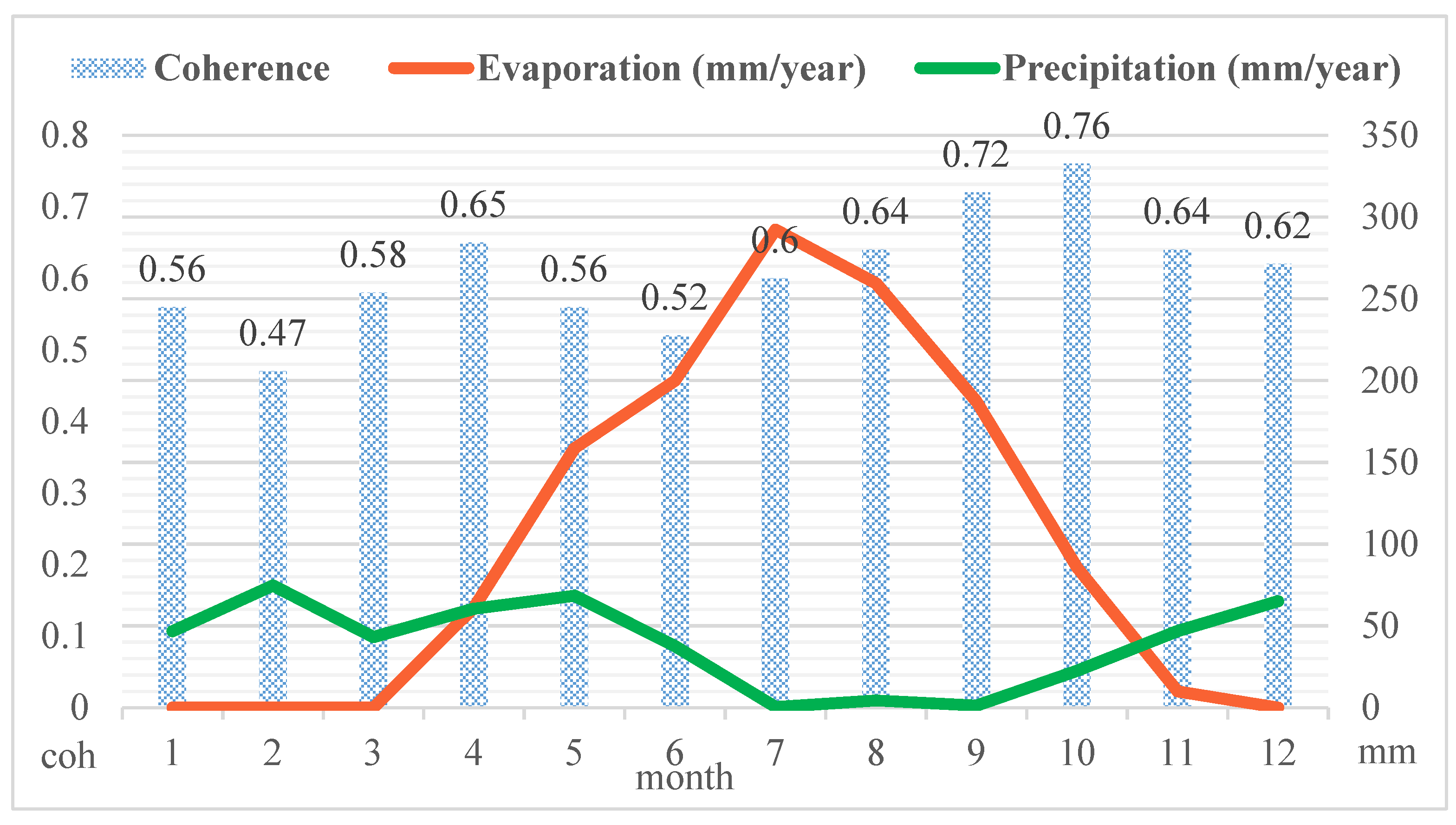
Additionally, to understand the impact of weather conditions on the coherence values, Figure 9 shows the monthly mean coherence values with monthly precipitation and evaporation, taken from four nearby meteorology stations: Aksaray, Cihanbeyli, Eskil, and Kulu. (see Figure 1).
In July, August, and October, when there was almost no rain, a decrease in coherence values was observed with the increase of evaporation. From November to March, when evaporation was almost absent, inversely proportional behavior between precipitation data and coherence data was observed. Even though there are temporal relations among the coherence, precipitation and evaporation (Figure 9), the meteorological effects on the temporal decorrelation can be ignored due to the presence of dense scatters satisfying the coherence condition (>0.45). This shows that the weather conditions had almost no effect on the C-band SBAS results for the study area, which should be greater on the shorter wavelength-based SBAS measurements.
Although the summer months are dry, there is no a major change in soil moisture because the lake is fed by underground water sources. In the field surveys, it was observed that the top layer of the soil was dry when the moisture rate was about 40% at 1.5–2 cm below the soil. The moisture content of soil samples taken from different parts of Lake Tuz was calculated. A negative linear correlation was observed between the backscattering value of Sentinel-1 images and soil moisture. Additionally, increases in soil moisture content result in a decrease in coherence values. Along with surface roughness, this feature is a disadvantage in moist areas, such as Lake Tuz, where evaporation occurs due to the salt concentration.
A brief evaluation of the coherence results can be found in Figure 10, which shows the total area of the assigned classes for each Sentinel-2 acquisition date. In the figure, colors distinguish the salt lake components, while the darker shade of each color describes the total area with a coherence value of greater than 0.45 within each component. These data produced for four different periods also show how these data were affected by seasonal changes.
It is seen that approximately 90% of the salt and dry soil classes, 70% of the moist soil, 65% of the vegetation classes, and 25% of the water class can be used for SBAS-based volume dynamics monitoring.
Relationships between the meteorological data in Figure 9 and Figure 10 were examined and a countertrend was observed. It was determined that evaporation mostly affects the salt class, while the class least affected by evaporation is dry soil. Precipitation mostly affects the water class negatively. It was observed that the reliable data of the water class, which was 27.20% in the dry season, decreased to 19.52% despite the increase in total water area due to precipitation.
4. Discussions
The joint analysis of SBAS and auxiliary data (in situ) results provides further insight into how the activities on site have an impact on the measurements from SBAS.
For this purpose, SBAS and levelling measurements were firstly compared in order to investigate the accuracy and reliability of the water level determination. Afterwards, the deformation results within the salt pans were analyzed to understand the potential of Sentinel-1 to seasonally monitor the salt pan volume dynamics. The results, obtained in a coordinated manner with GPS/leveling measurements and the SBAS results georeferenced according to GPS measurements, were matched. The displacement results were projected onto the vertical unit vector using the incident angle (33.86°). The SBAS results were then calibrated using the TUTGA points obtained and found homogeneously in the study area. Thus, the SBAS results were converted into levelling information and compared with the levelling information obtained in the field work. A total of 50 points were selected in the field survey area with water along the levelling line. A 20-meter diameter buffer was applied to each levelling point. The mean SBAS result in this area was compared with the levelling measurements. The total SBAS area used across the 50 levelling points was 1275 m2. Figure 11 compares the water level information obtained by the levelling measurements in four different seasons with water level information obtained from SBAS. The same points are used every season, and points with a water level of zero were not included in the process. The standard deviation values obtained from the SBAS accuracy comparisons in February, April, August and October were calculated as 0.67, 0.80, 0.84, and 0.95, respectively.
A lower correlation is observed between the two sets of data in February, when the water level reached a depth of 25 cm. This value increases as the water level decreases and the salt content in the water increases. When determining the water level at a depth of 25 cm, deviations of up to 7 cm can be seen as a result of SBAS. This difference decreases to 2–3 cm at 15 cm water depth, and to 0–1 cm at a depth of 8 cm. In addition, statistical analyses show that the root mean square error (RMSE) decreases as the water level of the lake decreases. RMSE values were calculated as 2.85 mm in February, 2.5 mm in April, 1.5 mm in July, and 0.5 mm in October (when the water level was the lowest). The salt class is one of the major dynamic classes among the components of a salt lake. To determine the volume dynamics in the salt class, the common salt class areas seen in the classifications of the lake in February, April, August, and October were selected for this study.
After examining the SBAS measurements corresponding to water level changes, SBAS-based surface changes within the salt pans were analyzed. One of the most important components of a salt lake is salt, which contributes to the country’s economy. It can be seen that salt formation, caused by the effect of evaporation, starts in April and lasts until September. Subsequently, with the rains, a collapse is observed, depending on the dissolution of the salt. To calculate the salt reserves in Lake Tuz, the (thickness) x (area) x (density) formula was used [48]. As shown in Figure 1, there are three active salt pans in the lake. There are negative and positive movements in saltpans due to the formation movements of salt. In order to make a more accurate salt yield calculation, DS candidates with coherence values greater than 0.6 in the vertical unit were determined, and their average values were calculated. Since these DS candidates were determined in the months before the salt harvest period, they were not exposed to any external factors. The values obtained from here were calculated as salt thickness, the total areas of the salt fields, and salt density were included in the process, and the salt yield was calculated. The salt yield was calculated by including the values obtained from here as salt thickness, the total areas of the salt fields, and the salt density.
Yavsan salt pan is located to the west of the lake and has an operating capacity of approximately 8.5 km2. The salt thickness was determined as 7.69 cm using the mean value of the SBAS results obtained in approximately 5.2 km2 of this area, and the salt yield calculation was made, giving a result of 1.438 million tons (Figure 12).
Kayacık salt pan is located to the east of the lake and has an operating capacity of approximately 11 km2. Salt thickness was determined as 7.51 cm using the mean value of the SBAS results obtained in approximately 4.8 km2 of this area and a salt yield calculation was made, giving a result of 1.838 million tons (Figure 13).
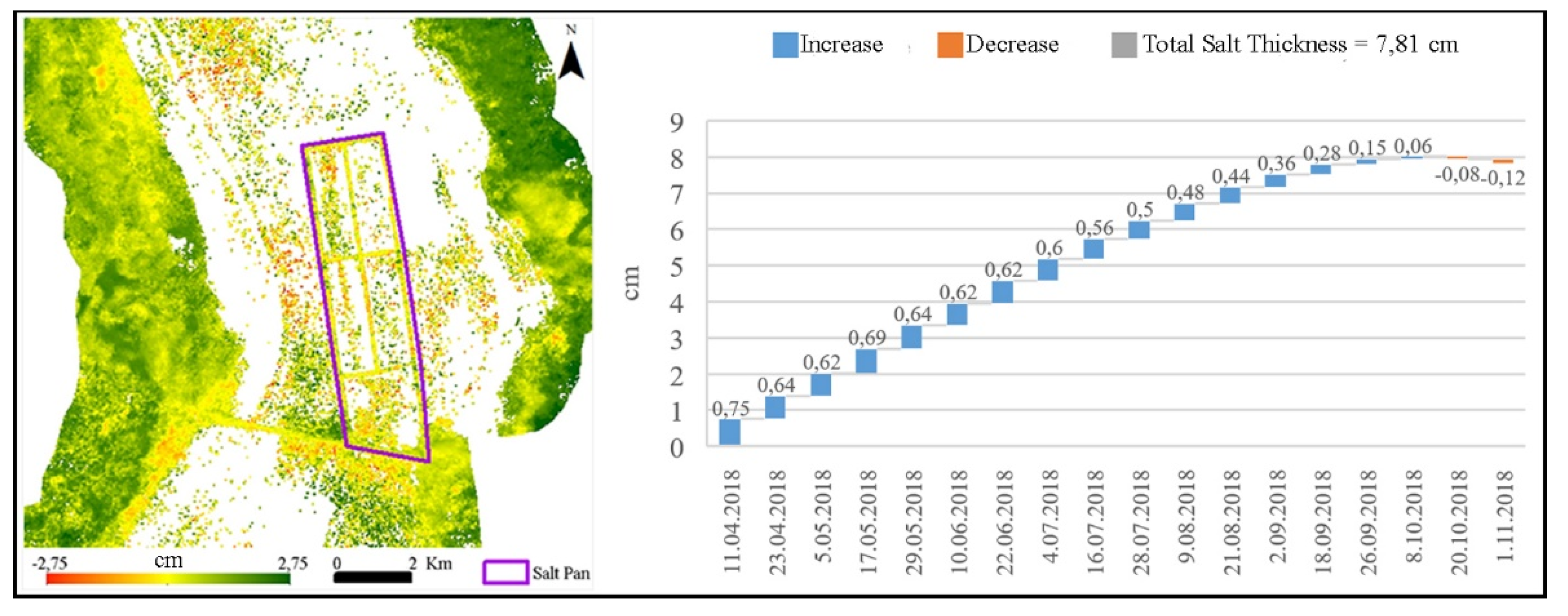
Kaldırım salt pan is located to the north of the lake and has an operating capacity of approximately 12 km2. Total salt thickness was determined as 7.81 cm using the mean value of the SBAS results obtained in approximately 6.1 km2 of this area, and a salt yield calculation was made, giving a result of 1.95 million tons (Figure 14).
5. Conclusions
In this study, the potential of freely available interferometric stacks of Sentinel-1 data, coupled with SBAS methodology, was evaluated as a way to monitor volume dynamics in a salt lake environment. To achieve this, the interferometric stacking technique was applied to 34 C-band VV polarized images taken over Lake Tuz in an annual period. SBAS measurement points, namely distributed scatterers which could be attributed to salt lake activities were monitored to understand the water-surface movement. These SBAS-based surface movements were in line with in situ measurements of water level change. The regression analysis showed a good fit, with an accuracy of 1–5 cm between the SBAS-based and the in situ measurements which exported vertical units, underlining the potential of freely available Sentinel-1 data to detect surface water level and salt lake components. Three salt pans in the lake were investigated to examine the movements of salt, clearly one of the most important components of salt lakes. It was seen that the thickness of the salt emerging under the effect of evaporation, starting in April, reached approximately 4 cm. The amount of salt production was calculated using the thickness of salt, and revealed an average of 5 million tons throughout the lake. This figure coincides with the number given by the salt businesses.
The impact of seasonal changes on the SBAS measurements was analyzed, showing coherence with the methodological data and Sentinel-2 images. A negative correlation was found between evapotranspiration and coherence values, which determines the quality of the measurements. Even though the variance of coherence values was high due to the high evapotranspiration from late August to the end of October, the mean coherence over the lake was always higher than 0.7, excluding pure water surfaces. The Sentinel-2 images were then used to study the relationship between the quality of SBAS measurements and dynamic salt lake components (water, vegetation, moist soil, dry soil, and salt) in the context of coherence measurements. In the summer season, although the highest decrease due to evaporation was in the salt and moist soil classes, this value did not fall below 0.7 in the salt class, or below 0.5 in the moist soil class. On the other hand, in the water class, it reached higher values with the increase of salt content in water following evaporation.
As a final remark, it should be emphasized that the SBAS method can be used for observation of the volume dynamics of salt lakes as there is no vegetation and they have highly reflective classes. It was seen in the study that in order to get good results in wetlands, the interferogram pairs to be used in the SBAS process were a perpendicular baseline below 100 meters and a temporal baseline below 30 days. In addition, it was observed that sufficient data can be obtained to extract information, even in the water class due to its salt content. The SBAS method has proved suitable for monitoring the volume dynamics of components, such as water level and salt movements, in salt lakes. The NASA–ISRO Synthetic Aperture Radar (NISAR) mission, which will provide data to its users in both the L band and the S band, will make an important contribution to volume dynamics and water level for future works.
Author Contributions
Conceptualization, N.M.; methodology, B.B.B. and E.E.; software, B.B.B.; validation, B.B.B., E.E. and N.M.; formal analysis, B.B.B.; investigation, B.B.B. and E.E.; resources, B.B.B.; data curation, B.B.B.; writing—original draft preparation, B.B.B.; writing—review and editing, E.E. and N.M.; visuali-zation, B.B.B.; supervision, E.E. and N.M.; project administration, N.M. All authors have read and agreed to the published version of the manuscript.
Funding
ITU BAP Project number MGA-2017-40803.
Institutional Review Board Statement
Not applicable.
Informed Consent Statement
Not applicable.
Data Availability Statement
Data sharing not applicable.
Acknowledgments
The authors would like to express their thanks to Istanbul Technical University (ITU), Scientific Research Project Funding for their financial support to ITU BAP Project number MGA-2017-40803.Also thank the European Space Agency (ESA) for providing SAR images (Sentinel-1) and grateful to Harris Geospatial Solutions for providing the SARscape software.
Conflicts of Interest
The authors declare no conflict of interest.
References
- Messager, M.L.; Lehner, B.; Grill, G.; Nedeva, I.; Schmitt, O. Estimating the volume and age of water stored in global lakes using a geo-statistical approach. Nat. Commun. 2016, 7, 13603. [Google Scholar] [CrossRef]
- Pedersen, E.; Weisner, S.E.; Johansson, M. Wetland areas’ direct contributions to residents’ well-being entitle them to high cultural ecosystem values. Sci. Total Environ. 2019, 646, 1315–1326. [Google Scholar] [CrossRef]
- Canisius, F.; Brisco, B.; Murnaghan, K.; Van Der Kooij, M.; Keizer, E. SAR backscatter and InSAR coherence for monitoring wetland extent, flood pulse and vegetation: A study of the Amazon lowland. Remote Sens. 2019, 11, 720. [Google Scholar] [CrossRef] [Green Version]
- Tiner, R.W. Wetlands: An Overview. In Remote Sensing of Wetlands: Applications and Advances, 1st ed.; Tiner, R.W., Lang, M.W., Klemas, V.V., Eds.; CRC Press: Boca Raton, FL, USA, 2015; pp. 3–18. [Google Scholar]
- Ding, X.; Li, X. Monitoring of the water-area variations of Lake Dongting in China with ENVISAT ASAR images. Int. J. Appl. Earth Obs. Geoinf. 2011, 13, 894–901. [Google Scholar] [CrossRef]
- Hu, S.; Niu, Z.; Chen, Y.; Li, L.; Zhang, H. Global wetlands: Potential distribution, wetland loss, and status. Sci. Total Environ. 2017, 586, 319–327. [Google Scholar] [CrossRef]
- Rezaeianzadeh, M.; Kalin, L.; Hantush, M.M. An Integrated Approach for Modeling Wetland Water Level: Application to a Headwater Wetland in Coastal Alabama, USA. Water 2018, 10, 879. [Google Scholar] [CrossRef] [Green Version]
- Van der Valk, A.G.; Volin, J.C.; Wetzel, P.R. Predicted changes in interannual water level fluctuations due to climate change and its implications for the vegetation of the Florida Everglades. Environ. Manag. 2015, 55, 799–806. [Google Scholar] [CrossRef] [PubMed]
- Liao, H.; Wdowinski, S.; Li, S. Regional-scale hydrological monitoring of wetlands with Sentinel-1 InSAR observations: Case study of the South Florida Everglades. Remote Sens. Environ. 2020, 251, 112051. [Google Scholar] [CrossRef]
- Hong, S.H.; Wdowinski, S.; Kim, S.W. Evaluation of TerraSAR-X observations for wetland InSAR application. IEEE Trans. Geosci. Remote Sens. 2010, 48, 864–873. [Google Scholar] [CrossRef]
- Schwatke, C.; Dettmering, D.; Bosch, W.; Seitz, F. DAHITI-an innovative approach for estimating water level time series over inland waters using multi-mission satellite altimetry. Hydrol. Earth Syst. Sci. 2015, 19, 4345–4364. [Google Scholar] [CrossRef] [Green Version]
- Yagmur, N.; Bilgilioglu, B.B.; Dervisoglu, A.; Musaoglu, N.; Tanik, A. Long and short–term assessment of surface area changes in saline and freshwater lakes via remote sensing. Water Environ. J. 2020, 35, 107–122. [Google Scholar] [CrossRef]
- Woodcock, C.E.; Allen, R.; Anderson, M.; Belward, A.; Bindschadler, R.; Cohen, W.B.; Gao, F.; Goward, S.N.; Helder, D.; Helmer, E.; et al. Free access to Landsat imagery. Sci. VOL 2008, 320, 1011. [Google Scholar] [CrossRef] [PubMed]
- Copernicus. Copernicus in Detail. Available online: https://www.copernicus.eu/en/about-copernicus/copernicus-detail (accessed on 10 February 2021).
- Calò, F.; Abdikan, S.; Görüm, T.; Pepe, A.; Kiliç, H.; Balik Şanli, F. The space-borne SBAS-DInSAR technique as a supporting tool for sustainable urban policies: The case of Istanbul Megacity, Turkey. Remote Sens. 2015, 7, 16519–16536. [Google Scholar] [CrossRef] [Green Version]
- Halicioglu, K.; Erten, E.; Rossi, C. Monitoring deformations of Istanbul metro line stations through Sentinel-1 and levelling observations. Environ. Earth Sci. 2021, 80, 361. [Google Scholar] [CrossRef]
- Bioresita, F.; Puissant, A.; Stumpf, A.; Malet, J.P. A method for automatic and rapid mapping of water surfaces from Sentinel-1 imagery. Remote Sens. 2018, 10, 217. [Google Scholar] [CrossRef] [Green Version]
- Imamoglu, M.; Kahraman, F.; Cakir, Z.; Sanli, F.B. Ground deformation analysis of Bolvadin (W. Turkey) by means of Multi-Temporal InSAR techniques and Sentinel-1 data. Remote Sens. 2019, 11, 1069. [Google Scholar] [CrossRef] [Green Version]
- Rotta, L.H.S.; Alcantara, E.; Park, E.; Negri, R.G.; Lin, Y.N.; Bernardo, N.; Mendes, T.S.G.; Souza Filho, C.R. The 2019 Brumadinho tailings dam collapse: Possible cause and impacts of the worst human and environmental disaster in Brazil. Int. J. Appl. Earth Obs. Geoinf. 2020, 90, 102119. [Google Scholar] [CrossRef]
- Orhan, O.; Oliver-Cabrera, T.; Wdowinski, S.; Yalvac, S.; Yakar, M. Land Subsidence and Its Relations with Sinkhole Activity in Karapınar Region, Turkey: A Multi-Sensor InSAR Time Series Study. Sensors 2021, 21, 774. [Google Scholar] [CrossRef]
- Drusch, M.; Del Bello, U.; Carlier, S.; Colin, O.; Fernandez, V.; Gascon, F.; Hoersch, B.; Isola, C.; Laberinti, P.; Martimort, P.; et al. Sentinel-2: ESA’s optical high-resolution mission for GMES operational services. Remote Sens. Environ. 2012, 120, 25–36. [Google Scholar] [CrossRef]
- Astola, H.; Häme, T.; Sirro, L.; Molinier, M.; Kilpi, J. Comparison of Sentinel-2 and Landsat 8 imagery for forest variable prediction in boreal region. Remote Sens. Environ. 2019, 223, 257–273. [Google Scholar] [CrossRef]
- D’Odorico, P.; Gonsamo, A.; Damm, A.; Schaepman, M.E. Experimental Evaluation of Sentinel-2 Spectral Response Functions for NDVI Time-Series Continuity. IEEE Trans. Geosci. Remote. Sens. 2013, 51, 1336–1348. [Google Scholar] [CrossRef]
- A24 Hedley, J.D.; Roelfsema, C.; Brando, V.; Giardino, C.; Kutser, T.; Phinn, S.; Mumby, P.J.; Barrilero, O.; Laporte, J.; Koetz, B. Coral reef applications of Sentinel-2: Coverage, characteristics, bathymetry and benthic mapping with comparison to Landsat 8. Remote. Sens. Environ. 2018, 216, 598–614. [Google Scholar] [CrossRef]
- Veloso, A.; Mermoz, S.; Bouvet, A.; Le Toan, T.; Planells, M.; Dejoux, J.F.; Ceschia, E. Understanding the temporal behavior of crops using Sentinel-1 and Sentinel-2-like data for agricultural applications. Remote Sens. Environ. 2017, 199, 415–426. [Google Scholar] [CrossRef]
- Mahdianpari, M.; Salehi, B.; Mohammadimanesh, F.; Homayouni, S.; Gill, E. The first wetland inventory map of newfoundland at a spatial resolution of 10 m using Sentinel-1 and Sentinel-2 data on the google earth engine cloud computing platform. Remote Sens. 2019, 11, 43. [Google Scholar] [CrossRef] [Green Version]
- Slagter, B.; Tsendbazar, N.E.; Vollrath, A.; Reiche, J. Mapping wetland characteristics using temporally dense Sentinel-1 and Sentinel-2 data: A case study in the St. Lucia wetlands, South Africa. Int. J. Appl. Earth Obs. Geoinf. 2020, 86, 102009. [Google Scholar] [CrossRef]
- Shi, X.; Yang, C.; Zhang, L.; Jiang, H.; Liao, M.; Zhang, L.; Liu, X. Mapping and characterizing displacements of active loess slopes along the upstream Yellow River with multi-temporal InSAR datasets. Sci. Total Environ. 2019, 674, 200–210. [Google Scholar] [CrossRef]
- Ferretti, A.; Prati, C.; Rocca, F. Permanent scatterers in SAR interferometry. IEEE Trans. Geosci. Remote Sens. 2001, 39, 8–20. [Google Scholar] [CrossRef]
- Erten, E.; Rossi, C. The worsening impacts of land reclamation assessed with Sentinel-1: The Rize (Turkey) test case. Int. J. Appl. Earth Obs. Geoinf. 2019, 74, 57–64. [Google Scholar] [CrossRef]
- Du, Z.; Ge, L.; Ng, A.H.M.; Zhu, Q.; Horgan, F.G.; Zhang, Q. Risk assessment for tailings dams in Brumadinho of Brazil using InSAR time series approach. Sci. Total Environ. 2020, 717, 137125. [Google Scholar] [CrossRef] [PubMed]
- Selvakumaran, S.; Rossi, C.; Barton, E.; Middleton, C.R. Interferometric Synthetic Aperture Radar (InSAR) in the Context of Bridge Monitoring. In Advances in Remote Sensing for Infrastructure Monitoring, 1st ed.; Singhroy, V., Ed.; Springer: Cham, Germany, 2020; pp. 183–209. [Google Scholar]
- Ciampalini, A.; Solari, L.; Giannecchini, R.; Galanti, Y.; Moretti, S. Evaluation of subsidence induced by long-lasting buildings load using InSAR technique and geotechnical data: The case study of a Freight Terminal (Tuscany, Italy). Int. J. Appl. Earth Obs. Geoinf. 2019, 82, 101925. [Google Scholar] [CrossRef]
- Xie, C.; Xu, J.; Shao, Y.; Cui, B.; Goel, K.; Zhang, Y.; Yuan, M. Long term detection of water depth changes of coastal wetlands in the Yellow River Delta based on distributed scatterer interferometry. Remote Sens. Environ. 2015, 164, 238–253. [Google Scholar] [CrossRef] [Green Version]
- Berardino, P.; Fornaro, G.; Lanari, R.; Sansosti, E. A new algorithm for surface deformation monitoring based on small baseline differential SAR interferograms. IEEE Trans. Geosci. Remote Sens. 2002, 40, 2375–2383. [Google Scholar] [CrossRef] [Green Version]
- Osmanoğlu, B.; Sunar, F.; Wdowinski, S.; Cabral-Cano, E. Time series analysis of InSAR data: Methods and trends. ISPRS J. Photogramm. Remote Sens. 2016, 115, 90–102. [Google Scholar] [CrossRef]
- Orhan, O. Monitoring of land subsidence due to excessive groundwater extraction using small baseline subset technique in Konya, Turkey. Environ. Monit. Assess. 2021, 193, 174. [Google Scholar] [CrossRef] [PubMed]
- Caló, F.; Notti, D.; Galve, J.P.; Abdikan, S.; Görüm, T.; Pepe, A.; Balik Şanli, F. Dinsar-Based detection of land subsidence and correlation with groundwater depletion in Konya Plain, Turkey. Remote Sens. 2017, 9, 83. [Google Scholar] [CrossRef] [Green Version]
- Chen, Z.; White, L.; Banks, S.; Behnamian, A.; Montpetit, B.; Pasher, J.; Duffe, J.; Bernard, D. Characterizing marsh wetlands in the Great Lakes Basin with C-band InSAR observations. Remote Sens. Environ. 2020, 242, 111750. [Google Scholar] [CrossRef]
- Xiang, W.; Zhang, R.; Liu, G.; Wang, X.; Mao, W.; Zhang, B.; Bao, J.; Cai, J.; Fu, Y. Extraction and analysis of saline soil deformation in the Qarhan Salt Lake region (in Qinghai, China) by the sentinel SBAS-InSAR technique. Geod. Geodyn. 2021. Available online: https://www.sciencedirect.com/science/article/pii/S1674984720300859 (accessed on 5 January 2021).
- Hong, S.H.; Wdowinski, S.; Kim, S.W.; Won, J.S. Multi-temporal monitoring of wetland water levels in the Florida Everglades using interferometric synthetic aperture radar (InSAR). Remote Sens. Environ. 2010, 114, 2436–2447. [Google Scholar] [CrossRef]
- Kaya, Z. Potential natural heritage sites in Turkey. In World Heritage, 1st ed.; Rössle, M., Ed.; DL Services: Sint Pieters Leeuw, Belgium, 2016; Volume 80, pp. 84–89. [Google Scholar]
- Ekercin, S.; Ormeci, C. Estimating soil salinity using satellite remote sensing data and real-time field sampling. Environ. Eng. Sci. 2008, 25, 981–988. [Google Scholar] [CrossRef]
- Orhan, O.; Dadaser-Celik, F.; Ekercin, S. Investigating land surface temperature changes using Landsat-5 data and real-time infrared thermometer measurements at Konya closed basin in Turkey. Int. J. Eng. Geosci. 2019, 4, 16–27. [Google Scholar]
- Kilic, O.; Kilic, A.M. Salt crust mineralogy and geochemical evolution of the salt lake (Tuz Gölü), Turkey. Sci. Res. Essays 2010, 5, 1317–1324. [Google Scholar]
- Ozfidan-Konakci, C.; Uzilday, B.; Ozgur, R.; Yildiztugay, E.; Sekmen, A.H.; Turkan, I. Halophytes as a source of salt tolerance genes and mechanisms: A case study for the Salt Lake area, Turkey. Funct. Plant Biol. 2016, 43, 575–589. [Google Scholar] [CrossRef]
- TVKGM. Lake Tuz Special Protection Area Management Plan 2014–2018. Available online: https://webdosya.csb.gov.tr/db/tabiat/editordosya/tuz%20golu-4(2).pdf (accessed on 8 February 2021).
- Köylü, M.K. Salt Lake’s Financial Investment Value and Its Contribution to Economic Growth. Int. J. Acad. Value Stud. 2017, 3, 127–137. [Google Scholar]
- Chen, Q.; Liu, X.; Zhang, Y.; Zhao, J.; Xu, Q.; Yang, Y.; Liu, G. A nonlinear inversion of InSAR-observed coseismic surface deformation for estimating variable fault dips in the 2008 Wenchuan earthquake. Int. J. Appl. Earth Obs. Geoinf. 2019, 76, 179–192. [Google Scholar] [CrossRef]
- Zhou, L.; Guo, J.; Hu, J.; Li, J.; Xu, Y.; Pan, Y.; Shi, M. Wuhan surface subsidence analysis in 2015–2016 based on Sentinel-1a data by SBAS-InSAR. Remote Sens. 2017, 9, 982. [Google Scholar] [CrossRef] [Green Version]
- ESA. User Guides Introduction. Available online: https://earth.esa.int/web/sentinel/user-guides (accessed on 10 February 2021).
- Hong, S.H.; Wdowinski, S. Evaluation of the quad-polarimetric Radarsat-2 observations for the wetland InSAR application. Can. J. Remote Sens. 2012, 37, 484–492. [Google Scholar] [CrossRef] [Green Version]
- Aslan, G.; Cakir, Z.; Lasserre, C.; Renard, F. Investigating subsidence in the Bursa Plain, Turkey, using ascending and descending Sentinel-1 satellite data. Remote Sens. 2019, 11, 85. [Google Scholar] [CrossRef] [Green Version]
- Tampuu, T.; Praks, J.; Uiboupin, R.; Kull, A. Long term interferometric temporal coherence and DInSAR phase in Northern Peatlands. Remote Sens. 2020, 12, 1566. [Google Scholar] [CrossRef]
- Wegmüller, U.; Magnard, C.; Werner, C.; Strozzi, T.; Caduff, R.; Manconi, A. Methods to avoid being affected by non-zero closure phase in InSAR time series analysis in a multi-reference stack. Procedia Comput. Sci. 2021, 181, 511–518. [Google Scholar] [CrossRef]
- Ormeci, C.; Ekercin, S. An assessment of water reserve changes in Salt Lake, Turkey, through multi–temporal Landsat imagery and real–time ground surveys. Hydrol. Process. Int. J. 2007, 21, 1424–1435. [Google Scholar] [CrossRef]
- Ekercin, S.; Örmeci, C. Evaluating climate change effects on water and salt resources in Salt Lake, Turkey using multitemporal SPOT imagery. Environ. Monit. Assess. 2010, 163, 361–368. [Google Scholar] [CrossRef] [PubMed]
- Orhan, O.; Yalvaç, S.; Ekercin, S. Investigation of climate change impact on Salt Lake by statistical methods. Int. J. Environ. Geoinformatics 2017, 4, 54–62. [Google Scholar] [CrossRef] [Green Version]
- Sica, Y.V.; Quintana, R.D.; Radeloff, V.C.; Gavier-Pizarro, G.I. Wetland loss due to land use change in the Lower Paraná River Delta, Argentina. Sci. Total Environ. 2016, 568, 967–978. [Google Scholar] [CrossRef] [PubMed]
- Judah, A.; Hu, B. The integration of multi-source remotely-sensed data in support of the classification of wetlands. Remote Sens. 2019, 11, 1537. [Google Scholar] [CrossRef] [Green Version]
- Pande-Chhetri, R.; Abd-Elrahman, A.; Liu, T.; Morton, J.; Wilhelm, V.L. Object-based classification of wetland vegetation using very high-resolution unmanned air system imagery. Eur. J. Remote Sens. 2017, 50, 564–576. [Google Scholar] [CrossRef] [Green Version]
Figure 1.
Geographic location of Lake Tuz overlaid on the hillside background, as well as the spatial distribution of the meteorological and hydrological stations and in situ areas used in this study. The reference area where the levelling measurement was carried out is enlarged.
Figure 1.
Geographic location of Lake Tuz overlaid on the hillside background, as well as the spatial distribution of the meteorological and hydrological stations and in situ areas used in this study. The reference area where the levelling measurement was carried out is enlarged.

Figure 2.
Workflow implemented for the water level monitoring.

Figure 3.
Temporal (x-axis) and perpendicular (y-axis) baseline of the Sentinel-1 acquisitions (red points). Individual SBAS interferogram pairs are shown by blue lines between every two different points.
Figure 3.
Temporal (x-axis) and perpendicular (y-axis) baseline of the Sentinel-1 acquisitions (red points). Individual SBAS interferogram pairs are shown by blue lines between every two different points.

Figure 4.
Spectral curves of the salt lake components from ASD, and spatial resolution of each of the spectral bands used from Sentinel-2.
Figure 4.
Spectral curves of the salt lake components from ASD, and spatial resolution of each of the spectral bands used from Sentinel-2.

Figure 5.
Examples of levelling measurements during wet and dry season (The left picture shows a 9 cm water depth; the right picture shows the salt surface.).
Figure 5.
Examples of levelling measurements during wet and dry season (The left picture shows a 9 cm water depth; the right picture shows the salt surface.).

Figure 6.
SBAS LOS direction velocity map for the 2017–2018 period. The final map is presented by cutting Lake Tuz and its surroundings (approximately 1900 km2). Positive velocities (in green) represent the motion of the ground toward the satellite, while negative velocities (in red) represent motion away from the satellite (a). The spatial distribution of the standard deviation of the SBAS measurements (b). Photographs taken around Lake Tuz which have different structures (c).

Figure 7.
(a,b) Sentinel-2 classified images and the corresponding Sentinel-1 coherence images derived from the seasonal data. Coherence maps of shortest time-based interferograms containing selected Sentinel-2 images.
Figure 7.
(a,b) Sentinel-2 classified images and the corresponding Sentinel-1 coherence images derived from the seasonal data. Coherence maps of shortest time-based interferograms containing selected Sentinel-2 images.

Figure 8.
Boxplot of all coherence values of different LULC classes for four different seasons. Each feature is described by its classes and different seasons. Each table contains the class names and statistical info.
Figure 8.
Boxplot of all coherence values of different LULC classes for four different seasons. Each feature is described by its classes and different seasons. Each table contains the class names and statistical info.

Figure 9.
Average monthly precipitation, evapotranspiration and coherence. Meteorological data were obtained by mean value of Kulu, Cihanbeyli, Eskil and S. Kochisar stations around the lake.
Figure 9.
Average monthly precipitation, evapotranspiration and coherence. Meteorological data were obtained by mean value of Kulu, Cihanbeyli, Eskil and S. Kochisar stations around the lake.

Figure 10.
The total area of each of the Lake Tuz components in time (see Figure 7). The areas with a coherence value greater than 0.45 within these classes are shown in a darker color.
Figure 10.
The total area of each of the Lake Tuz components in time (see Figure 7). The areas with a coherence value greater than 0.45 within these classes are shown in a darker color.

Figure 11.
Regression analysis between water levels derived by SBAS that exported vertical units and levelling.
Figure 11.
Regression analysis between water levels derived by SBAS that exported vertical units and levelling.

Figure 12.
Salt movements obtained by SBAS results. The location of the salt pan is shown on the LOS directions SBAS map in the left image, while the change in the salt height in this salt pan is graphically displayed on the right (Calculations were made by converting to vertical units).
Figure 12.
Salt movements obtained by SBAS results. The location of the salt pan is shown on the LOS directions SBAS map in the left image, while the change in the salt height in this salt pan is graphically displayed on the right (Calculations were made by converting to vertical units).

Figure 13.
Salt movements obtained by SBAS results. The location of the salt pan is shown on the LOS directions SBAS map in the left image, while the change in the salt height in this salt pan is graphically displayed on the right (Calculations were made by converting to vertical units).
Figure 13.
Salt movements obtained by SBAS results. The location of the salt pan is shown on the LOS directions SBAS map in the left image, while the change in the salt height in this salt pan is graphically displayed on the right (Calculations were made by converting to vertical units).

Figure 14.
Salt movements obtained by SBAS results. The location of the salt pan is shown on the LOS direction SBAS map in the left image, while the change in the salt height in this salt pan is graphically displayed on the right (Calculations were made by converting to vertical units).
Figure 14.
Salt movements obtained by SBAS results. The location of the salt pan is shown on the LOS direction SBAS map in the left image, while the change in the salt height in this salt pan is graphically displayed on the right (Calculations were made by converting to vertical units).


Table 1.
Properties of Sentinel-1/-2. Text highlighted in * refers to the chosen features.
| Satellite (Optical) | Spectral Res. (µm) | Spatial Res. (m) | Rad. Res. (bit) | Temp. Res. (Day) |
|---|---|---|---|---|
| Sentinel 2 MSI | 13 Bands (0.44–2.20) | * B2, B3, B4, B8:10 m * B5, B6, B7, B8a, B11, B12:20m B1, B9, B10: 60 m | 12 | 5 |
| Satellite (SAR) | Polarization * | Spatial Res. (m) | Incidence Angle (°) | Temp. Res. (Day) |
| Sentinel-1 (C band) | HH, HV, * VV, VH | 5 (ground range) × 20 (azimuth) | 29.1°–46.0° | 6 |
Publisher’s Note: MDPI stays neutral with regard to jurisdictional claims in published maps and institutional affiliations. |
© 2021 by the authors. Licensee MDPI, Basel, Switzerland. This article is an open access article distributed under the terms and conditions of the Creative Commons Attribution (CC BY) license (https://creativecommons.org/licenses/by/4.0/).
Share and Cite
MDPI and ACS Style
Bilgilioğlu, B.B.; Erten, E.; Musaoğlu, N. Analysis of Salt Lake Volume Dynamics Using Sentinel-1 Based SBAS Measurements: A Case Study of Lake Tuz, Turkey. Remote Sens. 2021, 13, 2701. https://doi.org/10.3390/rs13142701
AMA Style
Bilgilioğlu BB, Erten E, Musaoğlu N. Analysis of Salt Lake Volume Dynamics Using Sentinel-1 Based SBAS Measurements: A Case Study of Lake Tuz, Turkey. Remote Sensing. 2021; 13(14):2701. https://doi.org/10.3390/rs13142701
Chicago/Turabian StyleBilgilioğlu, Burhan Baha, Esra Erten, and Nebiye Musaoğlu. 2021. "Analysis of Salt Lake Volume Dynamics Using Sentinel-1 Based SBAS Measurements: A Case Study of Lake Tuz, Turkey" Remote Sensing 13, no. 14: 2701. https://doi.org/10.3390/rs13142701
Note that from the first issue of 2016, this journal uses article numbers instead of page numbers. See further details here.