Article

Urban Sprawl and Changes in Land-Use Efficiency in the Beijing–Tianjin–Hebei Region, China from 2000 to 2020: A Spatiotemporal Analysis Using Earth Observation Data

1
College of Geological Engineering and Geomatics, Chang’an University, Xi’an 710054, China
2
Key Laboratory of Digital Earth Science, Aerospace Information Research Institute, Chinese Academy of Sciences, Beijing 100094, China
3
Center for Urban and Environmental Change, Department of Earth and Environmental Systems, Indiana State University, Terre Haute, IN 47809, USA
4
School of Geomatics and Urban Spatial Informatics, Beijing University of Civil Engineering and Architecture, Beijing 102616, China
5
Airborne Remote Sensing Center, Aerospace Information Research Institute, Chinese Academy of Sciences, Beijing 100094, China
*
Author to whom correspondence should be addressed.
Remote Sens. 2021, 13(15), 2850; https://doi.org/10.3390/rs13152850
Submission received: 2 June 2021 / Revised: 9 July 2021 / Accepted: 16 July 2021 / Published: 21 July 2021

Abstract

:
Sustainable development in urban areas is at the core of the implementation of the UN 2030 Agenda and the Sustainable Development Goals (SDG). Analysis of SDG indicator 11.3.1—Land-use efficiency based on functional urban boundaries—provides a globally harmonized avenue for tracking changes in urban settlements in different areas. In this study, a methodology was developed to map built-up areas using time-series of Landsat imagery on the Google Earth Engine cloud platform. By fusing the mapping results with four available land-cover products—GlobeLand30, GHS-Built, GAIA and GLC_FCS-2020—a new built-up area product (BTH_BU) was generated for the Beijing–Tianjin–Hebei (BTH) region, China for the time period 2000–2020. Using the BTH_BU product, functional urban boundaries were created, and changes in the size of the urban areas and their form were analyzed for the 13 cities in the BTH region from 2000 to 2020. Finally, the spatiotemporal dynamics of SDG 11.3.1 indicators were analyzed for these cities. The results showed that the urban built-up area could be extracted effectively using the BTH_BU method, giving an overall accuracy and kappa coefficient of 0.93 and 0.85, respectively. The overall ratio of the land consumption rate to population growth rate (LCRPGR) in the BTH region fluctuated from 1.142 in 2000–2005 to 0.946 in 2005–2010, 2.232 in 2010–2015 and 1.538 in 2015–2020. Diverged changing trends of LCRPGR values in cities with different population sizes in the study area. Apart from the megacities of Beijing and Tianjin, after 2010, the LCRPGR values were greater than 2 in all the cities in the region. The cities classed as either small or very small had the highest LCRPGR values; however, some of these cities, such as Chengde and Hengshui, experienced population loss in 2005–2010. To mitigate the negative impacts of low-density sprawl on environment and resources, local decision makers should optimize the utilization of land resources and improve land-use efficiency in cities, especially in the small cities in the BTH region.

Graphical Abstract

1. Introduction

According to the United Nations, at present, more than 4 billion people live in urban areas worldwide, and this number continues to rise [1]. The global urbanization trend lead to excessive land use change and expansion of urban land [2]. The physical growth of urban areas is often disproportionate in relation to population growth which results in inefficient land use. This type of growth contradicts the principle of sustainability by leading to several negative impacts such as fragmentation of agro-forest landscape, increase of energy consumption and carbon emission [3]. Therefore, the efficient use of land resources is crucial for urban sustainability from ecological and socioeconomic points of view [4].
Several indicators have been developed to examine the impact of urbanization on land resources [5]. In 2015, the United Nations set out 17 social, economic and environmental sustainable development goals and 169 specific targets in the Transforming Our World: The 2030 Agenda for Sustainable Development, which will guide the global development effort during the period 2015–2030 [6]. Among them, SDG indicator 11.3.1 measures urban land-use efficiency (LUE), which is the ratio of the rate of consumption of urban land to the rate of population growth [7]. The production and dissemination of the SDG 11.3.1 indicator can characterize the evolution of urban settlements. By monitoring the spatio-temporal changes in urban land use efficiency, city authorities and decision makers can identify new areas of growth and project demand for public goods and services. They can also formulate policies that encourage optimal use of urban land and effectively protect natural and agricultural lands. Therefore, the information of LUE evolution is necessary for providing adequate infrastructure and services for improving living conditions of urban residents, as well as preserving environmentally sensitive areas from development [4].
Previous studies of urban expansion and sprawl have mainly been based on administrative boundaries [8,9]. However, urban areas experienced an outward expansion exceeding their formal administrative boundaries in a large proportion of cities due to the poor urban and regional planning and land speculation [10]. A dynamic and functional definition of urban boundaries was proposed and applied in the LUE analysis framework produced by UN-Habitat [7]. The use of functional urban boundaries makes it possible to track changes across human settlements and provides a globally harmonized avenue for tracking changes in urban settlements in different areas [11]. Unlike administrative boundaries, the functional urban area is defined as actual areas where urban growth happens. Using spatial analysis approaches from the built environment measures extracted from satellite imagery, the functional urban area can be identified [7]. Hence, the LUE indicators can be measured using built-up area and population grid data within the boundary of functional urban area. The produced results can represent the actual prevailing growth trends in the city and provide accurate aggregates to better inform decision makers at local and national levels. The use of functional urban boundaries makes it possible to track changes across human settlements and provides a globally harmonized avenue for tracking changes in urban settlements in different areas [11].
By collecting a wide range of information about the planet at large spatial scales, remote sensing can complement traditional data sources to track progress in achieving sustainable development goals and targets [12]. In particular, the development of free and open remote sensing data and high-performance cloud-computing platforms has made it possible to map urban built-up areas or impervious surfaces using Earth Observation data at the global scale [13,14,15,16,17]. Urban land-cover products derived from remote sensing data have been used to monitor and assess SDG 11.3.1 trends at national and global scales. The free and open Global Human Settlement Layer data were used to estimate SDG 11.3.1 in approximately 10,000 urban centers globally from 1990 to 2015 [11,18]. Based on the 1990, 2000 and 2010 CLUDS datasets, DMSP/OLS night-light data and census data, the spatial heterogeneity and dynamic trend of urban expansion and population growth in mainland China during the period 1990–2010 were analyzed in combination with SDG 11.3.1 [19]. These efforts at LUE monitoring at different spatial scales confirmed the applicability of Earth Observation data for providing consistent information on urban SDG indicators and informing the formulation of urban land-use policy.
However, the accuracy of Earth observation products can vary between different regions, which can lead to uncertainties in evaluation results. Efforts have been made to measure LUE changes using satellite data at the local city scale. Using Landsat and SPOT images from 1996, 2001–2002 and 2011, the SDG 11.3.1 indicator was evaluated for four South African cities, and it was demonstrated that the population growth rate and rate of spatial expansion of small and second-tier cities in Africa was faster than that of large cities [20]. Ghazaryan et al. developed an automated classification approach and monitored urban sprawl and densification processes in western Germany using SDG Indicator 11.3.1 [21]. Spatiotemporal changes in urban land-use efficiency were analyzed and urban land lease policy gaps were emphasized to help ensure sustainable urban growth in fast-growing cities in Ethiopia [22].
Since the reform and opening up which began in 1978, China’s urbanization rate has increased from 17.9% in 1978 to 60.6% in 2019 [23]. This urbanization process is constantly accelerating and greatly promotes the nation’ s social and economic development. One results of the country’s industrialization and urbanization over the past four decades has been the gradual formation of large urban agglomerations or megalopolises [24,25]. The Beijing–Tianjin–Hebei (BTH) region is the largest such urban agglomeration in northern China. Monitoring and analyzing the dynamic changes in urban space is necessary to understand the urban development processes in this region. Therefore, the objectives of this study include: (1) to develop an approach to extract urban built-up areas by using Earth observation data; (2) to analyze urban expansion processes based on remote sensing products of built-up areas; and (3) to assess the spatial and temporal changes in urban land-use efficiency in the cities of the Beijing–Tianjin–Hebei urban agglomeration, China.

2. Study Area and Datasets

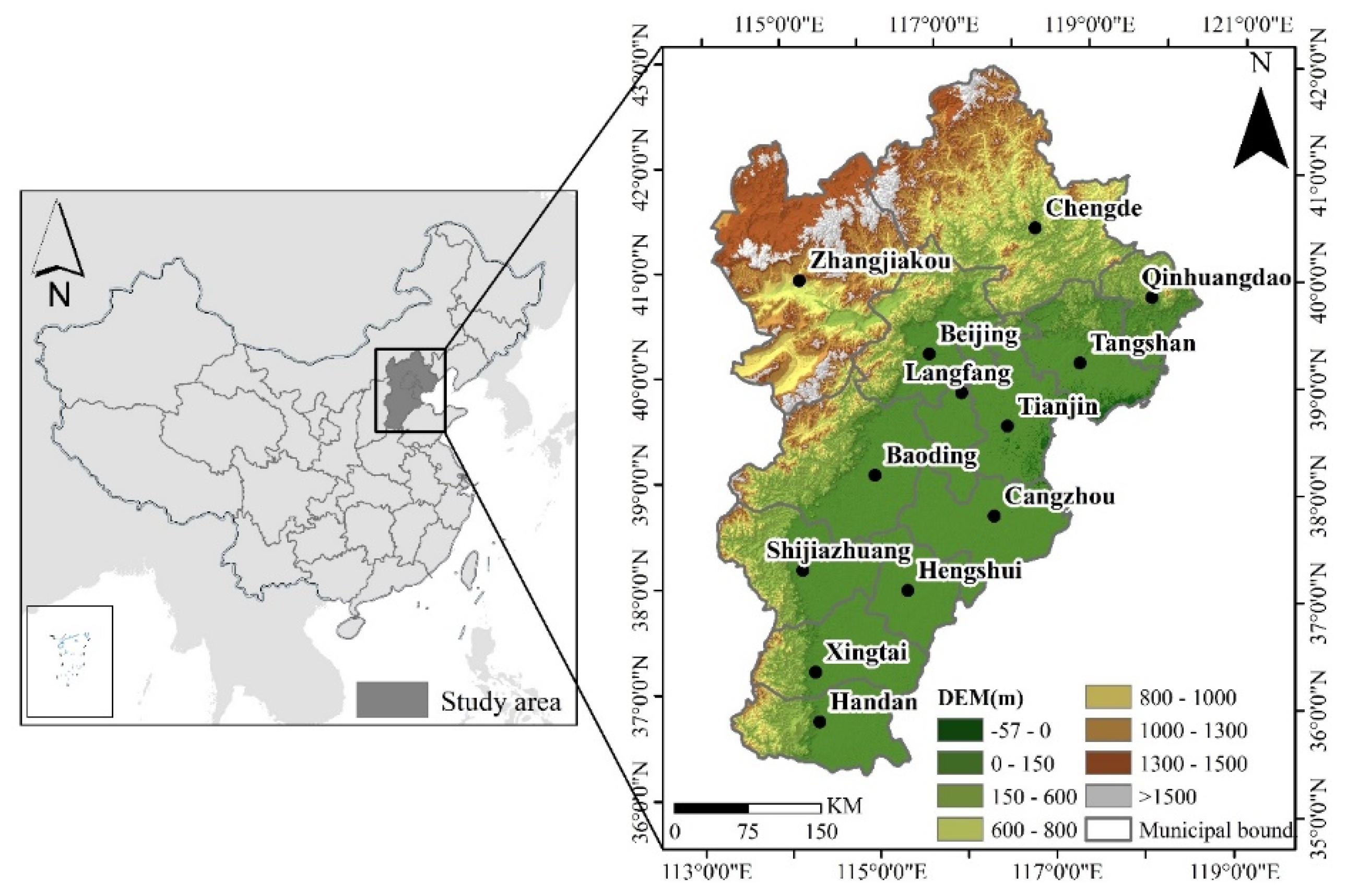
2.1. Beijing–Tianjin–Hebei Region

The Beijing-Tianjin-Hebei (BTH) region lies between the latitudes 36°03′ N and 42°40′ N and the longitudes 113°27′ E and 119°50′ E in northern China (Figure 1). It consists of Beijing and Tianjin municipalities, and 11 prefecture-level cities in Hebei Province (Zhangjiakou, Chengde, Qinhuangdao, Tangshan, Cangzhou, Hengshui, Langfang, Baoding, Shijiazhuang, Xingtai and Handan). Among them, Beijing and Tianjin are megacities with a population of more than 10 million. The area of this region comprises 218,000 km², accounting for 2.3% of China’s land area. The total population of the study area in 2020 is 113 million, accounting for 7.8% of China’s total population.
Since 2014, the coordinated development of the BTH region has become a major national strategic policy of China. As the center of economic development in the north of the country, the BTH region plays a significant role in China’s political and economic development [8]. To realize the coordinated development of the region and build a world-class urban agglomeration, the urbanization of the region should be developed in a planned and sustainable way, which requires timely monitoring of the processes and status of urban growth.

2.2. Datasets

The datasets used in this study included Landsat satellite images, topographic data, population data and administrative boundaries. Details of these datasets are described in the following sections.

2.2.1. Landsat Imagery

The Google Earth Engine (GEE), which can process satellite and other Earth observation data, is a cloud-based computing platform [26]. The platform stores nearly 40 years of publicly available global remote sensing images, including Landsat, Sentinel, MODIS and DMSP/OLS satellite imagery [27]. In this study, Landsat 5 tier-1 surface reflectance data from 2000, 2005 and 2010 and Landsat 8 data from 2015 and 2020 provided by the Google Earth Engine were used as the main data source for built-up area extraction. These datasets were atmospherically corrected using the GEE platform; this processing included cloud, shadow, water and snow masks.

2.2.2. Built-Up Area Products

Four urban built-up land or land-cover products were used in this study, including GlobeLand30, GAIA, GHS-Built and GLC_FCS-2020. These all have a spatial resolution of 30 m. The characteristics of these datasets are shown in Table 1.
The GAIA product is a global high-spatial-resolution (30 m) annual artificial surface dynamic data product (1985–2018) released in 2019. GAIA is produced using the Google Earth Engine platform together with long-time series of Landsat images (nearly 1.5 million scenes) as the main data source and auxiliary data such as night-light data and Sentinel-1 SAR data [28]. The GAIA dataset reveals the different rates of change in artificial impervious surface cover in major countries and regions of the world.
The Global Human Settlement Layer (GHSL) was developed by the Joint Research Centre (JRC) and contains spatial information about human settlements at a global scale [29]. The GHSL uses the core method of symbolic machine learning (SML) for data extraction and uses Landsat images from the past 40 years as the main data source. The GHSL is an open and free dataset. The GHS-Built product was used in this study. This product consists of multi-temporal data extracted from Landsat imagery (consisting of the GLS1975, GLS1990 and GLS2000 datasets and ad-hoc Landsat 8 data for 2013/2014). There are three types of land use classified in this product: built-up areas, non-built-up areas and water bodies.
The GLC_FCS30-2020 data is a global 30 m land-cover product with a fine classification system for the year 2020 [30]. The GLC_FCS30-2020 dataset is produced based on time-series of Landsat surface reflectance data (from 2019–2020), Sentinel-1 SAR data, DEM data, and auxiliary datasets. These data reflect the land cover types found globally (except for Antarctica) at a spatial resolution of 30 m in 2020.
The GlobeLand30 datasets from 2000, 2010 and 2020 were used in this study. These data include 10 land-cover types such as artificial land and bare land and cover the land within the range 80° S–80° N. The GlobeLand30 data were mainly classified using Landsat TM\ETM+ images and China Environmental Disaster Reduction Satellite (HJ-1) data based on a comprehensive pixel–object–knowledge classification method [31].
The data set used in this study are built-up area mapping results from these products. In the GAIA, GHS-Built, GLC_FCS30-2020, and GlobeLand30 products, the built-up areas are defined as impervious, built-up, impervious surfaces, and artificial surfaces, respectively. Hence, the four products are reclassified into two land cover types: non-built-up areas and built-up areas. The non-built-up area includes all other land cover types except built-up area, such as water, cropland, and forest. The specific reclassification schemes for each land cover product are shown in Table 2. In order to fuse theses datasets with the mapping results we derived using Google Earth Engine, the four built-up area products were re-projected to the same geo-reference system consisting of the WGS-84 coordinate system and UTM projection and resampled to a spatial resolution of 30 m.

2.2.3. Population Data

The WorldPop project, which is funded by the Bill & Melinda Gates Foundation, aims to offer spatial population datasets for Central and South America, Africa and Asia to support development, disaster response and health applications. The WorldPop data constitute an open-access gridded population data set (https://www.worldpop.org/ (10 April 2021)), produced by using a combination of machine learning and asymmetric modeling [32]. In this study, the population datasets for China for 2000, 2005, 2010, 2015 and 2020, which have a spatial resolution of 100 m and are based on the WGS84 geographic coordinate system, were used. The WorldPop population totals for different countries have been adjusted to match the corresponding official United Nations population estimates obtained from the Population Division of the Department of Economic and Social Affairs of the United Nations Secretariat.

2.2.4. Ancillary Datasets

The SRTM (Shuttle Radar Topography Mission) DEM is a digital elevation terrain model published by NASA and the National Bureau of Surveying and Mapping (NIMA). It has a spatial resolution of 30 m [33] and can be accessed directly in GEE. The administrative boundaries, including municipal district boundaries, provincial boundaries and municipal boundaries, can be obtained from National Geomatics Center of China (http://www.ngcc.cn/ngcc// (6 March 2021)).

3. Methodology

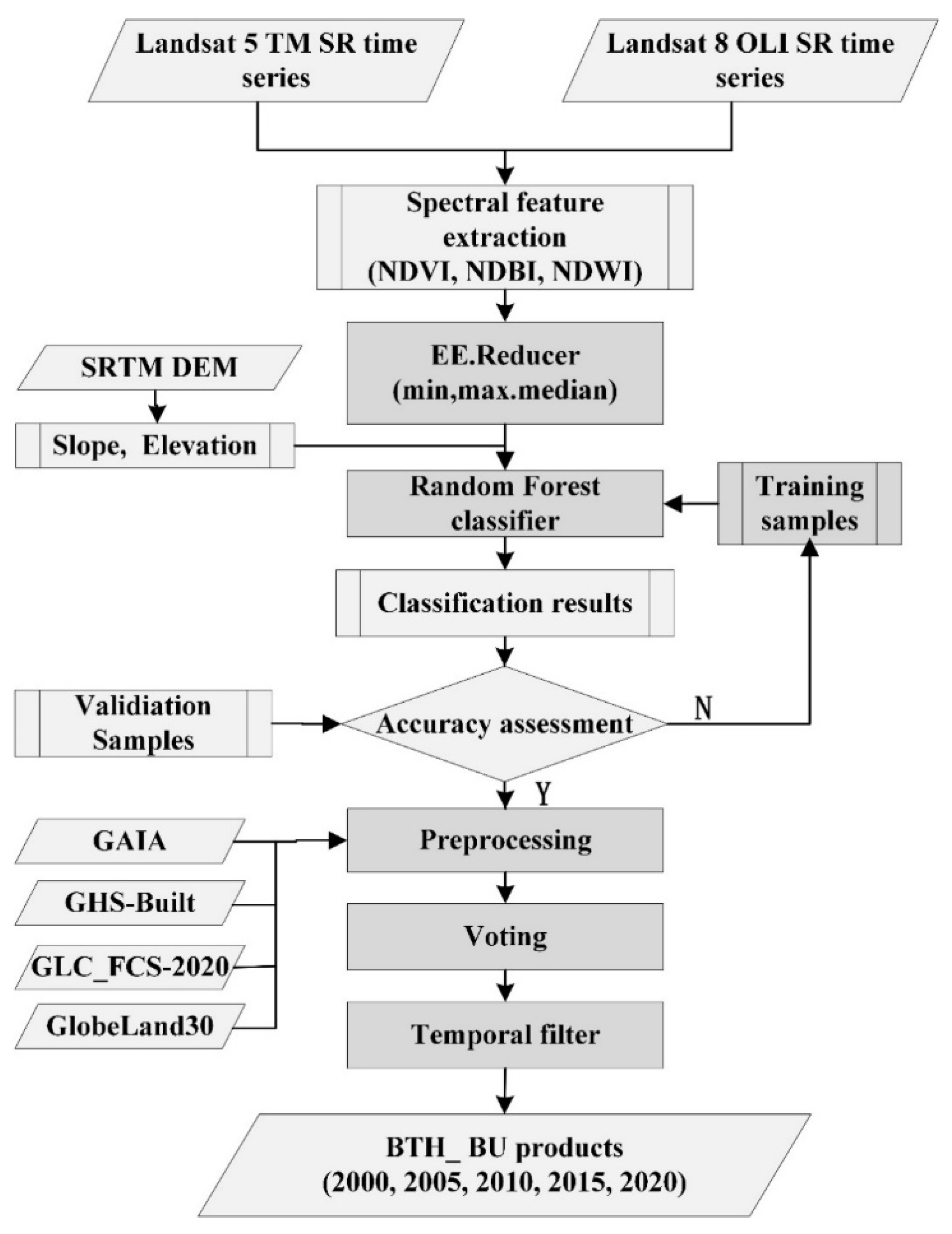
3.1. Built-Up Area Extraction

Three spectral indices—the normalized difference built-up index (NDBI), normalized difference vegetation index (NDVI) and normalized difference water index (NDWI)—were calculated from time-series of Landsat images [34,35,36]. Annual composite images were created from the optical, near-infrared, NDVI, NDBI and NDWI bands using the ‘reduce’ method by provided by GEE. The reduce method reduces a collection of images to an image by performing operation such as summation, median, etc. pixel by pixel. Four reduce functions—min, max, mean and median—were applied to improve the classification accuracy [37]. Sample points were selected by visual interpretation using the GEE platform. A stratified random sampling method was implemented with mapped land cover classes as strata [38]. The numbers of the sample points were determined based on the areal proportion of each land cover type. 80% of the sample points were randomly taken as training samples and 20% as validation sample points. Elevation and slope data calculated from the SRTM DEM were used as supplementary data; image classification was performed using the random forest algorithm(RFA) [39]. The number of classification trees in the random forest classifier is 500, and the remaining parameters are default. The confusion matrix between the validation samples and the classified products was calculated and the overall accuracy (OA) and kappa coefficients were obtained [40]. For the dichotomy of built-up area products (built-up area and non-built-up area) in this study, OA is the accuracy of the overall pixel being correctly classified, which can directly reflect the proportion of the correct classification. Kappa coefficient is a statistical index that can measure the balance of the correct classification of different categories. Omission error refers to the pixels belonging to the built-up area but classified as non-built-up area. Commission error refers to the pixels that is not built-up but is classified as built-up area. We tested different strategies for splitting the training and validation samples. If the classification result meets the requirement of OA > 0.85 and kappa > 0.8 [41,42], it was exported. The RFA was run iteratively and classification result with the highest OA was taken as the final output. The resolution of classification result was 30 m, and the spatial reference system was WGS-84 coordinate system and UTM projection.
The voting method is one of the most commonly used multi-classifier combination methods [43,44] in which the category with the most votes is taken as the final classification result. When multiple categories have the same number of votes, one of them is randomly selected as the final result. Based on the existing products for classifying urban built-up land and the classification results obtained from the RFA, a multi-temporal urban built-up area dataset was generated using the majority voting method. After the voting method had been applied, a temporal filtering method was used to ensure that the amount of built-up land in the product exhibited a growing trend [45]. A majority filter with a 3 × 3 window size was used to remove isolated pixels to obtain the final built-up area products with 30 m resolution, BTH_BU 2000, BTH_BU 2005, BTH_BU 2010, BTH_BU 2015 and BTH_BU 2020 [36]. The data-processing workflow is shown in Figure 2.

3.2. Accuracy Assessment

In order to confirm the feasibility of the BTH_BU product for urban expansion analysis across time, it is necessary to evaluate its thematic accuracy. In this study, confusion matrix was used to evaluate and compare the accuracy of the built-up area products [46,47,48]. The comparative analysis can also provide useful information for applications of these products in urban expansion and other fields. The confusion matrix compares the consistency of the land cover categories in the reference data and the data to be verified at a specific location, and then creates a two-dimensional table that compares the two (i.e., a confusion matrix). Based on this matrix, several different indices, including the overall accuracy (OA), kappa coefficient, omission error (OE) and misclassification error (CE), which can measure the accuracy of the product, can be calculated [49]. The equations used to calculate these indices are:
O A = T P + T N T P + F P + F N + T N
p e = ( T P + F N ) · ( T P + F P ) + ( F P + T N ) · ( F N + T N ) T P + F P + F N + T N
k a p p a = p o p e 1 p e
C E = F P T P + F P
O E = F N T P + F N
where TP = true positive, TN = true negative, FP = false positive, FN = false negative and P o = OA. In this study, a true positive result indicated that the built-up area pixels had been correctly extracted. A true negative indicated that image pixels considered to be non-built-up areas had been classified as not built-up areas. A false positive meant that image pixels that did not correspond to built-up areas had mistakenly been extracted, and a false negative meant that image pixels that did correspond to built-up areas had not been extracted.
A total of 300 points including 150 classed as built-up land and 150 classed as non-built-up land were randomly created for each city using ArcGIS 10.5 software (Esri, Redlands, CA, USA). High-resolution satellite images from Google Earth obtained in the same year as the Landsat data were used to identify the land-cover types corresponding to these random points manually. An accuracy evaluation database was then built and used to calculate the error matrix and accuracy assessment indicators.

3.3. Urban Growth Analysis

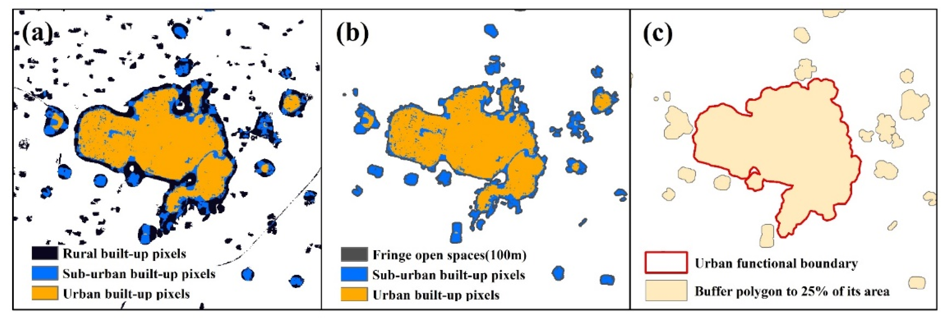
3.3.1. Functional City Boundary

Determining the extent of the built-up area is a prerequisite for measuring and comparing SDG 11.3.1. Instead of the administratively defined boundaries, the dynamic and functional urban boundary proposed by UN-Habitat—the actual area within which urban growth occurs over a defined period of time—was adopted in our study [10]. The functional urban boundary was obtained using several steps (Figure 3). The BTH_BU products are reclassified based on the density of built-up area per square kilometer. When the built-up area density is greater than 50%, it is defined as urban. If the built-up area density is greater than 0.25 and less than 0.5, it is defined as suburban. If the built-up area density is less than 0.25, it is considered as rural. The urban and suburban pixels were then used to determine the fringe open spaces, which are defined as areas within 100 m of urban and suburban pixels. A polygon was created by merging urban, sub-urban and the fringe open space pixels. Finally, buffer that extended the area of the polygon by 25% was created around each feature and the maximum extent of the buffer area was taken to be the functional urban boundary [7].

3.3.2. Change in Urban Built-Up Area

After obtaining the functional urban boundaries of the 13 cities in the study area in 2000, 2005, 2010, 2015 and 2020, the annual expansion area (AEA, km2) was used to quantify the amount and rate of urban expansion in our study [17]. The AE is defined as follows:
A E A = A end A start d
where Aend represents the urban built-up area at the end of a certain period, Astart is the built-up area at the beginning of a period and d is the number of years between the start and end of the period. The AEA can directly measure the annual change of built-up area and reveal the difference of the expansion amount of a city in different stages.

3.3.3. Change in Urban Form

The changes in urban form were analyzed by calculating compactness and aggregation indices which are spatial metrics. The compactness (C) of a city’s boundaries is an indicator that can reflect the form of the city’s space. It is defined as:
C = 2 π A / P
where C is the compactness of the city—that is, the compactness of the urban functional boundary. A is the area of the city and P denotes the length of the city perimeter. The greater the compactness value, the more compact the city is. A circle is the most compact shape: the compactness of a space in which each part is highly compressed is 1. In contrast, less compact shapes tend to be narrow or long. Also, the more complex a shape, the smaller its compactness.
The aggregation index (AI) of a city is defined as:
A I = ( g i i m a x g i i ) 100
where AI denotes the degree of aggregation and gii denotes the number of adjacent similar patches of the same landscape type. The AI is calculated based on the length of the common boundary between pixels corresponding to the same type of patch. When there is no common boundary between any of these pixels, the degree of aggregation is the lowest; when the common boundary between all pixels corresponding to the same type of patch reaches its maximum value, the aggregation index is the highest. In this study, the compactness and aggregation index for each built-up area, as defined by the functional urban boundaries, were calculated for each time period.

3.4. Derivation of LCR, PGR and LCRPGR

The SDG 11.3.1 indicators give the ratio of the land consumption rate (LCR) to the population growth rate (PGR). The PGR refers to the rate of population change in a city/urban area over a given period (usually a year). The LCR is defined as the rate of appropriation of land by urban development. The ratio of land consumption rate to population growth rate(LCRPGR) is calculated as the ratio of LCR to PGR. SDG 11.3.1 indicators are calculated using the following formulae:
L C R = ln ( U r b ( t + n ) / U r b t ) y ,
P G R = ln ( P o p ( t + n ) / P o p t ) y
L C R P G R = L C R P G R
where Popt is the total population of the urban area in the past/initial year, Pop(t+n) is the total population in the current/final year, Urbt is the total extent of the urban area (in km2) for the past/initial year, Urb(t+n) is the sum of the urban areas in the current/final year and y is the number of years between the two measurement periods.
Ideally, the ratio of land consumption to the population growth rate would be equal to 1, implying that the amount of urban land is increasing at the same rate as the population. Based on LCRPGR values, cities can be categorized into 5 types. These are shown in Table 3.

4. Results

4.1. Accuracy Assessment

Accuracy evaluation indices were obtained for each of these built-up area products for each study period (Table 4). Among the built-up area products, BTH_BU products had the highest average OA and Kappa coefficients and the lowest average OE and CE (Table 4). It shows that the proposed method can effectively improve the extraction accuracy of built-up area.
Figure 4 shows the OA, kappa coefficient, OE and CE of the five remote sensing products for each city. The classification accuracy of BTH_BU products in 11 out of 13 cities was the highest. BTH_BU and GlobeLand30 have the smallest variability in classification accuracy, followed by GLC_FCS and GHS-Built. GAIA has the largest variability in classification accuracy between the different cities.

4.2. Urban Growth Analysis

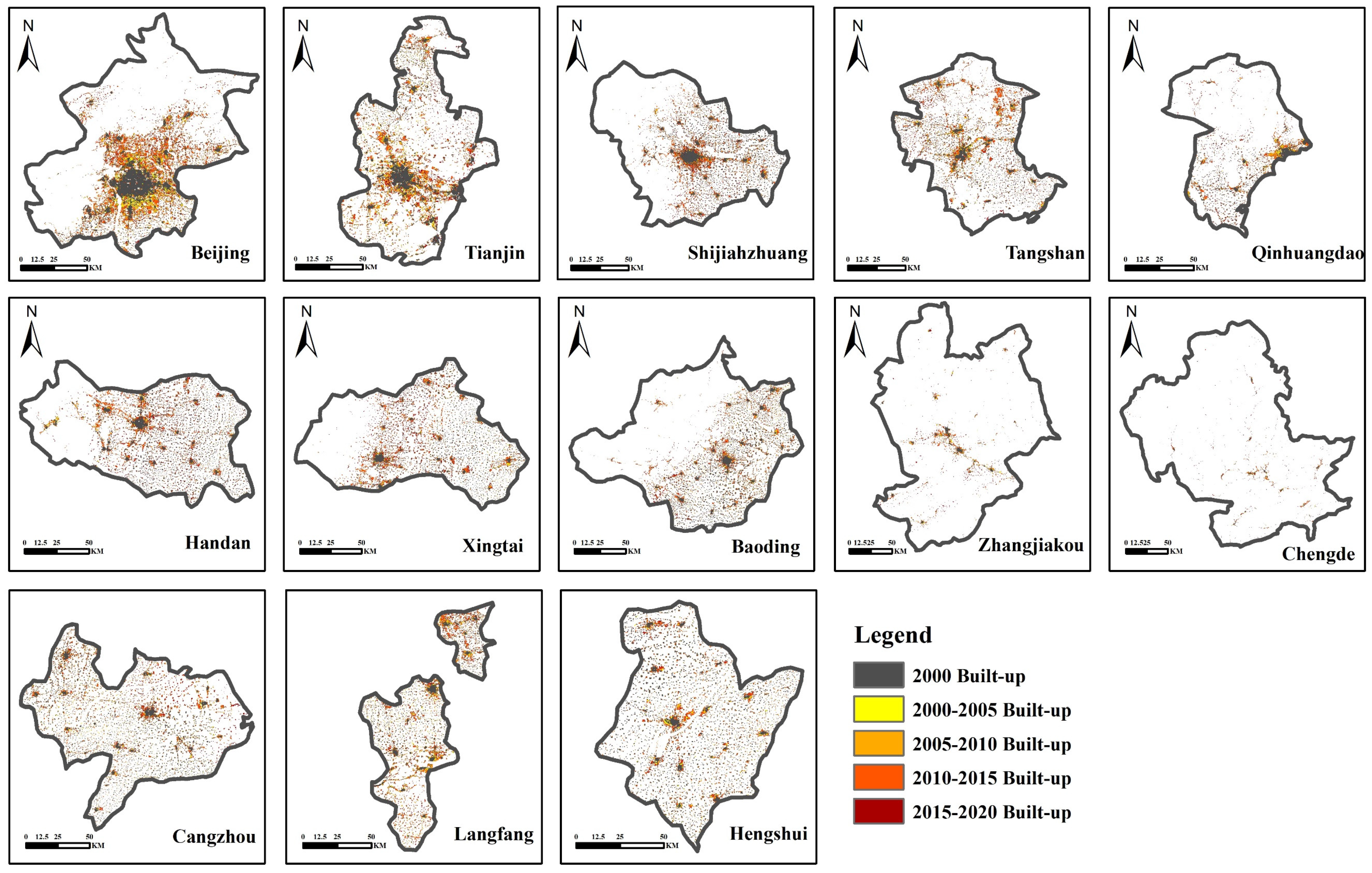
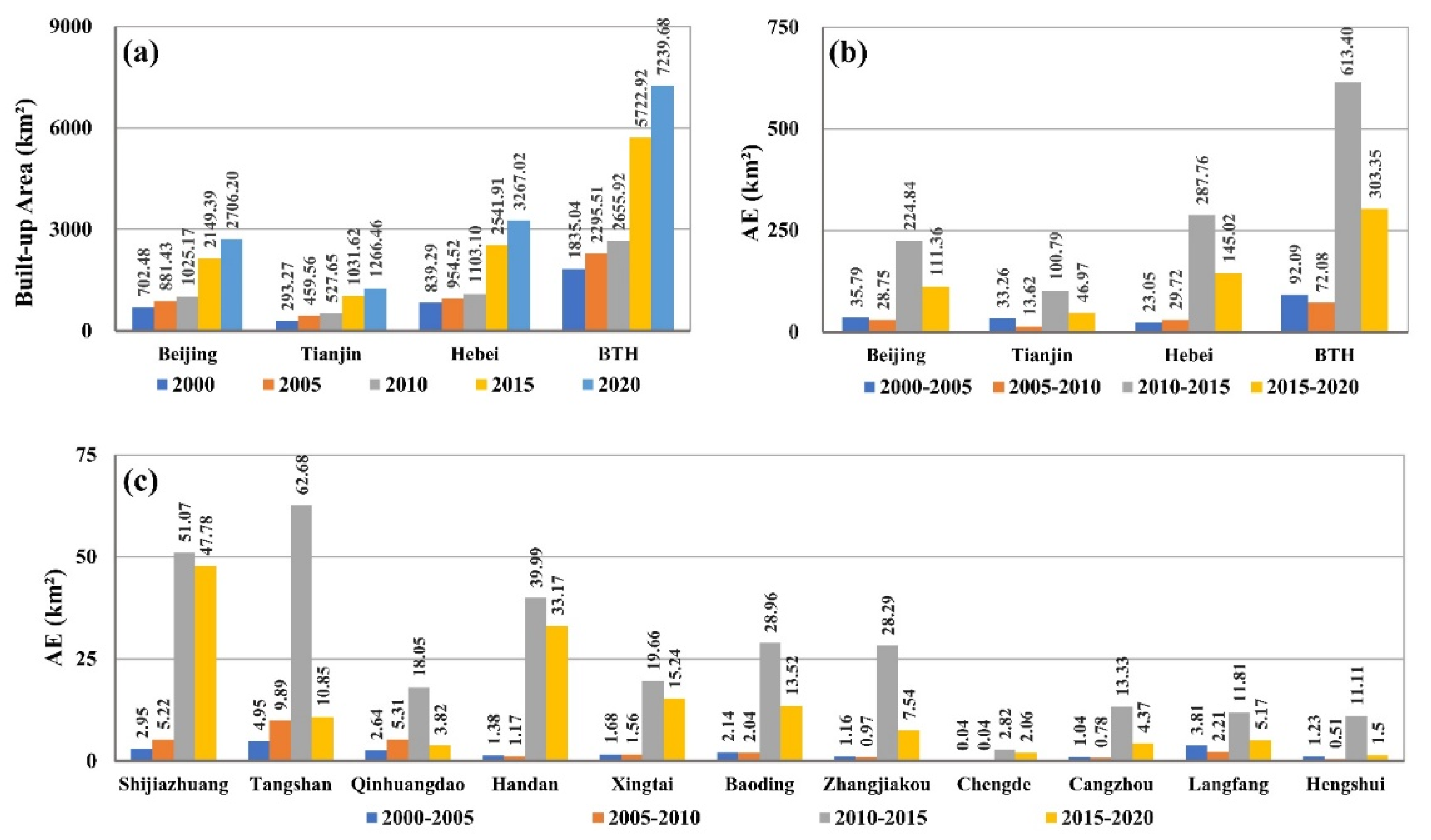
4.2.1. Changes in Urban Built-Up Area

Figure 5 shows the spatial pattern of urban expansion in the cities in the Beijing–Tianjin–Hebei region. Different types of urban spatial growth, infilling, edge-expansion, and leapfrogging, can be observed in these cities. The scattered built-up patches in suburban and rural areas was gradually connected with the central urban area, and thus forming a larger urban core in large cities.
The annual expansion area (AEA) of urban built-up area showed obvious regional differences (Figure 6). From 2010 to 2015, the AEA of the Beijing–Tianjin–Hebei built-up area is much higher than that in other periods. The dramatic changes in these values may indicate that a fusion between suburban patches and the core urban district or explosive growth resulting from the sprawl of built-up areas occurred during this period.

4.2.2. Changes in Urban Form

The changes in the compactness (C) and aggregation index (AI) for each city are shown in Figure 7. The compactness of all the cities in the Beijing–Tianjin–Hebei region shows a downward trend, while for the aggregation index (AI) there is an overall upward trend from 2000 to 2020 (Figure 7). The increasing trend in AI and the decreasing trend in C for all of the cities indicate that the built-up areas in all of these cities are gradually amalgamating and the spatial forms of the functional urban areas are becoming increasingly complex [50].

4.3. Spatiotemporal Dynamics of SDG 11.3.1

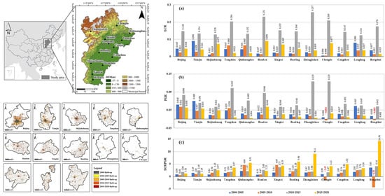
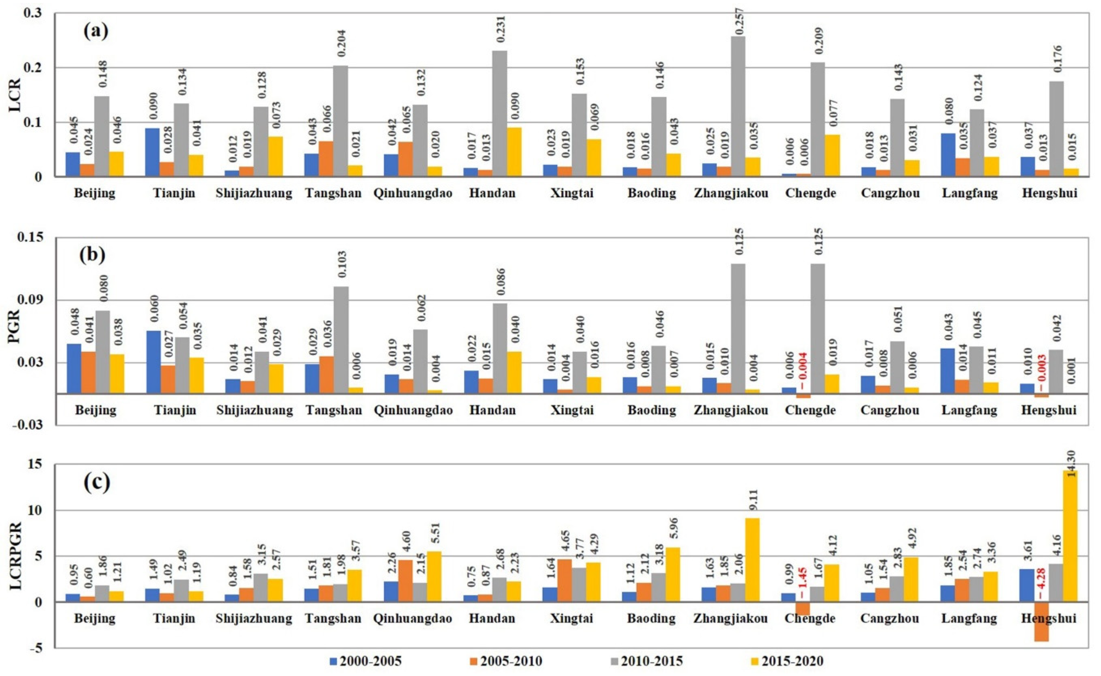
4.3.1. Variations in LCR, PGR and LCRPGR

The process of urbanization in the Beijing–Tianjin–Hebei region from 2000 to 2020 was analyzed by calculating the LCR, PGR and LCRPGR values (Table 5). The LCR, PGR and LCRPGR for the region all followed the same trend from 2000 to 2020: a decrease, followed by an increase, followed by another decrease. The decrease and increase in the LCRPGR during the period 2000–2015 agrees with the observed trend for all Chinese cities [51]. As a result of development in the early decades of the 21st century, there was also a consistent outward spread of the urban area in the Beijing–Tianjin–Hebei urban agglomeration. Before 2010, the rate of urban land growth was less than or similar to urbanization rate of the population. After Beijing hosted the Olympic Games in 2008, economic development led to rapid urban expansion in the Beijing–Tianjin–Hebei region. From 2010 to 2015, due to the acceleration in urban expansion and population growth, the LCR increased to 0.154, the PGR increased to 0.069 and the LCRPGR increased to 2.232. The urbanization rate of land was 2.232 times of the urbanization rate of population. In 2014, the National New Urbanization Plan (2014–2020) was issued by the national government and put forward a coordinated development strategy for the Beijing–Tianjin–Hebei region. As a guideline for China’s urbanization, the plan emphasized the importance of achieving a more environmentally and sustainable form of urbanization. During the period 2015–2020, the rate of increase in urban land and population urbanization slowed down, the LCR decreased to 0.048, the PGR decreased to 0.031 and the LCRPGR decreased to 1.538.
The temporal changes in the LCR, PGR and LCRPGR values of each city in the Beijing–Tianjin–Hebei region were analyzed. In the economically developed areas such as Beijing and Tianjin, the population growth and urban expansion were more rapid than in most cities in Hebei province. From 2000 to 2010 and from 2015 to 2020, although Beijing, as the capital of China, attracted a great inward flow of people, the rate of expansion of the built-up area was less than the population growth rate and the LCRPGR values were less than 1. Tianjin, the second largest city in the BTH region, had a higher LCRPGR value of between 1.0 and 1.5 (Figure 8). From 2010 to 2015, the built-up areas in all the cities in the Beijing–Tianjin–Hebei region expanded rapidly and their LCRPGR values were all greater than 1.5. The LCRPGR values for Langfang, Cangzhou, Baoding, Zhangjiakou and Tangshan have been increasing since 2000. By 2020, the LCRPGR values of these cities were all greater than 2, indicating that the cities had entered a phase of extensive development. In Qinhuangdao, the LCRPGR was greater than 2 during the period 2000–2020. Population growth in Hengshui has been relatively slow. The population growth here was negative from 2005 to 2010 and the absolute value of the LCRPGR from 2000 to 2020 was greater than 3. This indicates that a balance was maintained between the rates of urban expansion and population growth in Beijing and Tianjin. However, development in the cities in Hebei was unbalanced, with most of these cities underwent a phase of extensive development.

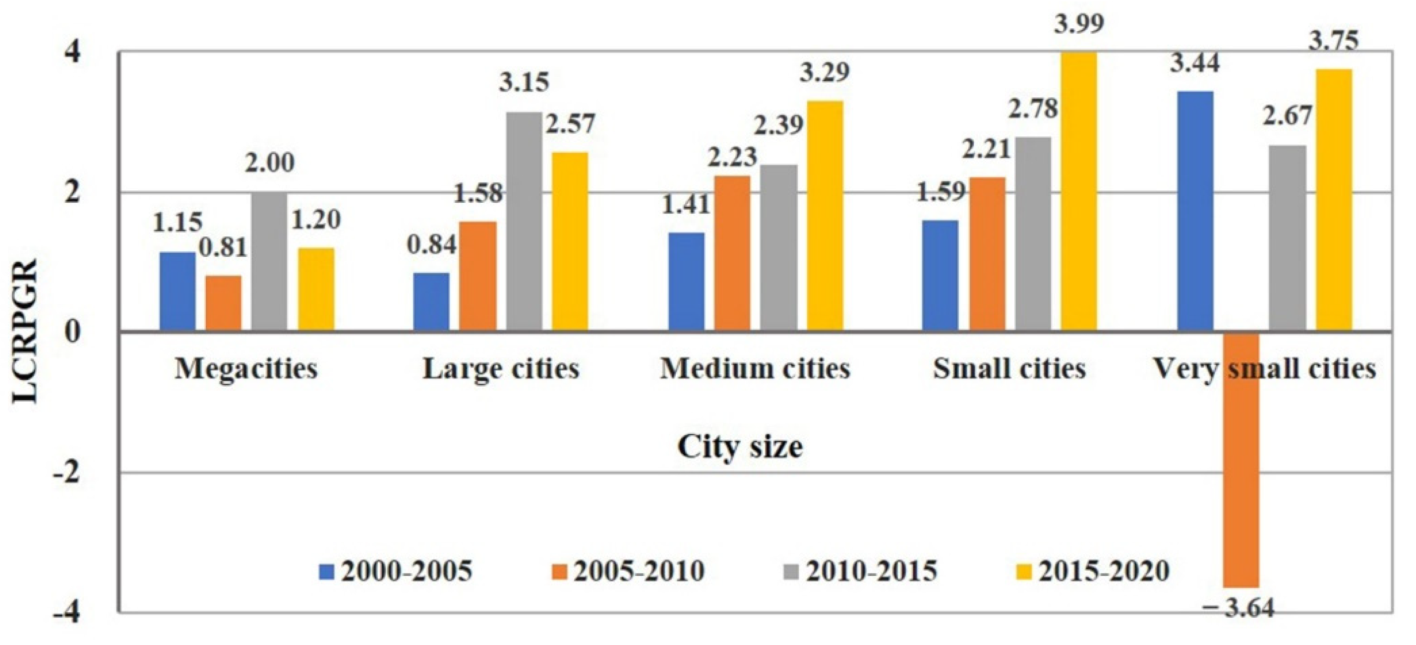
4.3.2. Differences in LCRPGR by City Type

We divided the 13 cities in the study into five categories based on population: very small cities, small cities, medium cities, large cities, and megacities (Table 6). The LCRPGR values for cities with different population sizes are shown in Figure 9.
Cities of different sizes undergone diverged urbanization processes during the study period (Figure 9). The LCRPGR values of megacities and large cities in 2015–2020 were lower than that before 2015, while the LCRPGR value of medium-sized cities, small cities and very small cities in 2015–2020 is higher than that before 2015. The slowed down sprawling development of megacities and large cities since 2015 might be attributed to the implementation of the new urbanization policy. However, the land use efficiency remains very low in medium, small and very small cities after 2015.

5. Discussion

5.1. Urban Growth Analysis

In this study, a new built-up area product (BTH_BU) was generated for the Beijing–Tianjin–Hebei (BTH) region by fusing the mapping results with four available land-cover products—GlobeLand30, GHS-Built, GAIA and GLC_FCS-2020. The accuracy of different built-up area or land cover products varies across cities. The accuracy of built-up area mapping mainly depends on the data sources, sample samples and classification methods employed. BTH_BU and GAIA rely mostly on the spectral features of Landsat data and a pixel-based classifier, whereas GHS-Built and GlobeLand30 also employ textural and contextual information about settlements that is obtained from remote sensing images. The GAIA and GLC_FCS-2020 uses both optical and Sentinel-1 SAR data. Our results showed that the integrative use of optical and SAR data improved the identification of buildings in less-dense urban areas. The sensitivity of SAR backscatter to building structures can help distinguish bare lands or sparse vegetated lands from built-up areas which are often confused in multispectral images [52]. By fusing the urban mapping results with four available products with a majority voting method, the BTH_BU takes advantage of different data products, and thus improved the accuracy of the final classification results.
Using the BTH_BU product and urban land use efficiency indicator, our results revealed diverged changing trends of LCRPGR values in cities with different population sizes in the study area. The extensive sprawling growth patterns in medium and small sized cities of this region suggest that economical and efficient use of land resources was neglected in urban planning and management strategies in these cities [17]. As the third largest urban agglomeration in China, the urban sprawl trajectory of cities with different sizes in Beijing–Tianjin–Hebei region can provide implications for other urban agglomerations [9]. Moreover, the urban mapping method and spatio-temporal urban sprawl analysis workflow using Earth observation data and geospatial technology can be applied to other cities and urban agglomerations.

5.2. Uncertainties and Limitations

Although the urban sprawl was characterized with the LCRPGR indicator effectively in our study, there are some limitations which should be considered. Multi-temporal Landsat imagery with 30 m spatial resolution was used as the main data source to extract urban land in this study, which limits the accuracy of built-up area extraction. The application of high resolution satellite data such as Sentinel-1/2, SPOT-5/6/7 and WorldView-2/3 may provide more detailed and accurate information on urban built-up areas [53,54]. For built-up area data fusion, different methods such as entropy weighting and performance weighting and the Dempster-Shafer theory can be applied in future studies [43]. When the LCRPGR value less than 0 is obtained, it should be interpreted with cautions. If PGR is less than 0 and LCR is greater than 0, the LCRPGR represents urban expansion and population loss. If PGR is greater than 0 and LCR is less than 0, it represents the decrease of built-up area and the increase of population in cities. Moreover, the indicators of SDG11.3.1 only use land and population as indicators, which may not fully characterize the urbanization process. Other environmental and economic indicators in SDGs can be used together with LCRPGR to perform a more comprehensive assessment of the urban development trajectories and trends.

6. Conclusions

In this study, a land-cover classification method was developed using a random forest classifier and Google Earth Engine cloud platform. The built-up area was extracted using time-series of Landsat imagery, a DEM and other ancillary data of the Beijing–Tianjin–Hebei region for the years 2000, 2005, 2010, 2015 and 2020. The data were also fused with four existing land-classification products—GlobeLand30, GHS-Built, GAIA and GLC_FCS-2020 to generate the built-up products BTH_BU 2000, BTH_BU 2005, BTH_BU 2010, BTH_BU 2015 and BTH_BU 2020. An accuracy assessment produced an overall accuracy of 0.93 and a kappa coefficient of 0.85 for the BTH_BU products. The built-up areas in all of these cities are aggregating and the spatial forms of the functional urban areas are becoming more complex. The spatiotemporal dynamics of the SDG 11.3.1 land-use efficiency indicators were monitored using BTH_BU and population data. The results showed that, for the BTH region overall, the LCRPGR values were close to 1 from 2000 to 2010 but rose to 2 or higher after 2010. Diverged changing trends of LCRPGR values in cities with different population sizes in the study area. The rates of land and population urbanization were found to be relatively balanced in the megacities of Beijing and Tianjin. Except for the megacities, the LCRPGR values were greater than 2 after 2010. The small and very small cities had the highest LCRPGR values after 2015; however, some of these cities, such as Chengde and Hengshui, experienced population loss. To mitigate the negative impacts of low-density sprawl on the environment and land resources, local decision makers should optimize the utilization of land resources and improve land-use efficiency in cities, especially in the small cities in the Beijing–Tianjin–Hebei region.

Author Contributions

Conceptualization: H.G. and L.L.; methodology: L.L.; software: L.L.; validation: M.Z. and S.Z.; formal analysis: M.Z.; investigation: S.C.; resources: Q.L.; data curation: M.Z.; original draft preparation: M.Z.; review and editing of draft: Q.W. and L.L.; visualization: M.Z.; supervision: L.L.; project administration: Q.L.; funding acquisition: Q.L. All authors have read and agreed to the published version of the manuscript.

Funding

This research was funded by the National Key Research and Development Program of China, grant number 2019YFE0127700; the National Natural Science Foundation of China, grant number 42071321; and the Strategic Priority Research Program of the Chinese Academy of Sciences, grant number XDA19030502.

Institutional Review Board Statement

Not applicable.

Informed Consent Statement

Not applicable.

Data Availability Statement

The data presented in this study are available on request from the corresponding author.

Acknowledgments

The authors would like to thank Yifang Ban from the KTH Royal Institute of Technology for her help regarding the SDG11.3.1 calculations. The authors are grateful for the constructive comments from anonymous reviewers and the editors.

Conflicts of Interest

The authors declare no conflict of interest.

References

  1. United Nations Department of Economic and Social Affairs. World Urbanization Prospects: The 2018 Revision (ST/ESA/SER.A/420). In Population Division; United Nations: New York, NY, USA, 2019. [Google Scholar]
  2. Grimm, N.B.; Faeth, S.H.; Golubiewski, N.E.; Redman, C.L.; Wu, J.; Bai, X.; Briggs, J.M. Global Change and the Ecology of Cities. Science 2008, 319, 756. [Google Scholar] [CrossRef] [Green Version]
  3. Jaeger, J.A.G.; Bertiller, R.; Schwick, C.; Cavens, D.; Kienast, F. Urban permeation of landscapes and sprawl per capita: New measures of urban sprawl. Ecol. Indic. 2010, 10, 427–441. [Google Scholar] [CrossRef]
  4. Zitti, M.; Ferrara, C.; Perini, L.; Carlucci, M.; Salvati, L. Long-Term Urban Growth and Land Use Efficiency in Southern Europe: Implications for Sustainable Land Management. Sustainability 2015, 7, 3359. [Google Scholar] [CrossRef] [Green Version]
  5. Hasse, J.E.; Lathrop, R.G. Land resource impact indicators of urban sprawl. Appl. Geogr. 2003, 23, 159–175. [Google Scholar] [CrossRef]
  6. Assembly, U.N.G. Transforming Our World: The 2030 Agenda for Sustainable Development A/RES/70/1; United Nations: New York, NY, USA, 2015. [Google Scholar]
  7. UN-Habitat. SDG Indicator 11.3.1 Training Module: Land Use Efficiency; UN-Habitat: Nairobi, Kenya, 2018. [Google Scholar]
  8. Haas, J.; Ban, Y. Urban growth and environmental impacts in Jing-Jin-Ji, the Yangtze, River Delta and the Pearl River Delta. Int. J. Appl. Earth Obs. Geoinf. 2014, 30, 42–55. [Google Scholar] [CrossRef]
  9. Sun, Y.; Zhao, S. Spatiotemporal dynamics of urban expansion in 13 cities across the Jing-Jin-Ji Urban Agglomeration from 1978 to 2015. Ecol. Indic. 2018, 87, 302–313. [Google Scholar] [CrossRef]
  10. UN-Habitat. Metadata on SDGs Indicator 11.3.1; UN-Habitat: Nairobi, Kenya, 2019. [Google Scholar]
  11. Melchiorri, M.; Pesaresi, M.; Florczyk, A.J.; Corbane, C.; Kemper, T. Principles and Applications of the Global Human Settlement Layer as Baseline for the Land Use Efficiency Indicator—SDG 11.3.1. ISPRS Int. J. Geo-Inf. 2019, 8, 96. [Google Scholar] [CrossRef] [Green Version]
  12. Anderson, K.; Ryan, B.; Sonntag, W.; Kavvada, A.; Friedl, L. Earth observation in service of the 2030 Agenda for Sustainable Development. Geo Spat. Inf. Sci. 2017, 20, 77–96. [Google Scholar] [CrossRef]
  13. Wu, B.; Tian, F.; Zhang, M.; Zeng, H.; Zeng, Y. Cloud services with big data provide a solution for monitoring and tracking sustainable development goals. Geogr. Sustain. 2020, 1, 25–32. [Google Scholar] [CrossRef]
  14. Li, W.; El-Askary, H.; Lakshmi, V.; Piechota, T.; Struppa, D. Earth Observation and Cloud Computing in Support of Two Sustainable Development Goals for the River Nile Watershed Countries. Remote Sens. 2020, 12, 1391. [Google Scholar] [CrossRef]
  15. Weng, Q. Remote sensing of impervious surfaces in the urban areas: Requirements, methods, and trends. Remote Sens. Environ. 2012, 117, 34–49. [Google Scholar] [CrossRef]
  16. Li, Q.; Lu, L.; Weng, Q.; Xie, Y.; Guo, H. Monitoring Urban Dynamics in the Southeast U.S.A. Using Time-Series DMSP/OLS Nightlight Imagery. Remote Sens. 2016, 8, 578. [Google Scholar] [CrossRef] [Green Version]
  17. Lu, L.; Guo, H.; Corbane, C.; Li, Q. Urban sprawl in provincial capital cities in China: Evidence from multi-temporal urban land products using Landsat data. Sci. Bull. 2019, 64, 955–957. [Google Scholar] [CrossRef] [Green Version]
  18. Pesaresi, M.; Huadong, G.; Blaes, X.; Ehrlich, D.; Ferri, S.; Gueguen, L.; Halkia, M.; Kauffmann, M.; Kemper, T.; Lu, L.; et al. A Global Human Settlement Layer From Optical HR/VHR RS Data: Concept and First Results. IEEE J. Sel. Top. Appl. Earth Observ. Remote Sens. 2013, 6, 2102–2131. [Google Scholar] [CrossRef]
  19. Wang, Y.C.; Huang, C.L.; Feng, Y.Y.; Zhao, M.Y.; Gu, J. Using Earth Observation for Monitoring SDG 11.3.1-Ratio of Land Consumption Rate to Population Growth Rate in Mainland China. Remote Sens. 2020, 12, 357. [Google Scholar] [CrossRef] [Green Version]
  20. Mudau, N.; Mwaniki, D.; Tsoeleng, L.; Mashalane, M.; Beguy, D.; Ndugwa, R. Assessment of SDG Indicator 11.3.1 and Urban Growth Trends of Major and Small Cities in South Africa. Sustainability 2020, 12, 7063. [Google Scholar] [CrossRef]
  21. Ghazaryan, G.; Rienow, A.; Oldenburg, C.; Thonfeld, F.; Trampnau, B.; Sticksel, S.; Jürgens, C. Monitoring of Urban Sprawl and Densification Processes in Western Germany in the Light of SDG Indicator 11.3.1 Based on an Automated Retrospective Classification Approach. Remote Sens. 2021, 13, 1694. [Google Scholar] [CrossRef]
  22. Koroso, N.H.; Zevenbergen, J.A.; Lengoiboni, M. Urban land use efficiency in Ethiopia: An assessment of urban land use sustainability in Addis Ababa. Land Use Policy 2020, 99, 105081. [Google Scholar] [CrossRef]
  23. National Bureau of Statistics of China. Statistical Communiqué of the People’s Republic of China on the 2019 National Economic and Social Development; National Bureau of Statistics of China: Beijing, China, 2020.
  24. Fang, C. Important progress and future direction of studies on China’s urban agglomerations. J. Geogr. Sci. 2015, 25, 1003–1024. [Google Scholar] [CrossRef] [Green Version]
  25. Fang, C.; Yu, D. Urban agglomeration: An evolving concept of an emerging phenomenon. Landsc. Urban Plan. 2017, 162, 126–136. [Google Scholar] [CrossRef]
  26. Moore, R.; Hansen, M. Google Earth Engine: A new cloud-computing platform for global-scale earth observation data and analysis. AGU Fall Meet. Abstr. 2011, 2011, IN43C-02. [Google Scholar]
  27. Gorelick, N.; Hancher, M.; Dixon, M.; Ilyushchenko, S.; Thau, D.; Moore, R. Google Earth Engine: Planetary-scale geospatial analysis for everyone. Remote Sens. Environ. 2017, 202, 18–27. [Google Scholar] [CrossRef]
  28. Gong, P.; Li, X.; Wang, J.; Bai, Y.; Chen, B.; Hu, T.; Liu, X.; Xu, B.; Yang, J.; Zhang, W.; et al. Annual maps of global artificial impervious area (GAIA) between 1985 and 2018. Remote Sens. Environ. 2020, 236. [Google Scholar] [CrossRef]
  29. Martino, P.; Daniele, E.; Stefano, F.; Aneta, F.; Vasileios, S. Operating procedure for the production of the Global Human Settlement Layer from Landsat data of the epochs 1975, 1990, 2000, and 2014. Publ. Off. Eur. Union 2016, 1–62. [Google Scholar]
  30. Zhang, X.; Liu, L.; Chen, X.; Gao, Y.; Xie, S.; Mi, J. GLC_FCS30: Global land-cover productwith fine classification system at 30 m using time-series Landsat imagery. Earth Syst. Sci. Data 2021, 13, 2753–2756. [Google Scholar] [CrossRef]
  31. Chen, J.; Chen, J.; Liao, A.; Cao, X.; Chen, L.; Chen, X.; He, C.; Han, G.; Peng, S.; Lu, M.; et al. Global land cover mapping at 30 m resolution: A POK-based operational approach. ISPRS J. Photogramm. Remote Sens. 2015, 103, 7–27. [Google Scholar] [CrossRef] [Green Version]
  32. Lloyd, C.T.; Sorichetta, A.; Tatem, A.J. High resolution global gridded data for use in population studies. Sci. Data 2017, 4, 170001. [Google Scholar] [CrossRef] [PubMed] [Green Version]
  33. Farr, T.G.; Kobrick, M. Shuttle radar topography mission produces a wealth of data. Eos Trans. Am. Geophys. Union 2000, 81. [Google Scholar] [CrossRef]
  34. Li, Q.; Lu, L.; Wang, C.; Li, Y.; Sui, Y.; Guo, H. MODIS-Derived Spatiotemporal Changes of Major Lake Surface Areas in Arid Xinjiang, China, 2000–2014. Water 2015, 7, 5731. [Google Scholar] [CrossRef]
  35. Lu, L.; Kuenzer, C.; Wang, C.; Guo, H.; Li, Q. Evaluation of Three MODIS-Derived Vegetation Index Time Series for Dryland Vegetation Dynamics Monitoring. Remote Sens. 2015, 7, 7597–7614. [Google Scholar] [CrossRef] [Green Version]
  36. Lu, L.; Weng, Q.; Xiao, D.; Guo, H.; Li, Q.; Hui, W. Spatiotemporal Variation of Surface Urban Heat Islands in Relation to Land Cover Composition and Configuration: A Multi-Scale Case Study of Xi’an, China. Remote Sens. 2020, 12, 2713. [Google Scholar] [CrossRef]
  37. Zhang, Z.; Wei, M.; Pu, D.; He, G.; Wang, G.; Long, T. Assessment of Annual Composite Images Obtained by Google Earth Engine for Urban Areas Mapping Using Random Forest. Remote Sens. 2021, 13, 748. [Google Scholar] [CrossRef]
  38. Olofsson, P.; Foody, G.M.; Herold, M.; Stehman, S.V.; Woodcock, C.E.; Wulder, M.A. Good practices for estimating area and assessing accuracy of land change. Remote Sens. Environ. 2014, 148, 42–57. [Google Scholar] [CrossRef]
  39. Breiman, L. Random Forests. Mach. Learn. 2001, 45, 5–32. [Google Scholar] [CrossRef] [Green Version]
  40. Foody, G.M. Status of land cover classification accuracy assessment. Remote Sens. Environ. 2002, 80, 185–201. [Google Scholar] [CrossRef]
  41. Kundel, H.L.; Polansky, M. Measurement of Observer Agreement. Radiology 2003, 228, 303–308. [Google Scholar] [CrossRef]
  42. Wickham, J.; Stehman, S.V.; Gass, L.; Dewitz, J.A.; Sorenson, D.G.; Granneman, B.J.; Poss, R.V.; Baer, L.A. Thematic accuracy assessment of the 2011 National Land Cover Database (NLCD). Remote Sens. Environ. 2017, 191, 328–341. [Google Scholar] [CrossRef] [Green Version]
  43. Zhang, H.; Xu, R. Exploring the optimal integration levels between SAR and optical data for better urban land cover mapping in the Pearl River Delta. Int. J. Appl. Earth Obs. Geoinf. 2018, 64, 87–95. [Google Scholar] [CrossRef]
  44. Smits, P.C. Multiple classifier systems for supervised remote sensing image classification based on dynamic classifier selection. IEEE Trans. Geosci. Remote Sens. 2002, 40, 801–813. [Google Scholar] [CrossRef]
  45. Zhang, L.; Weng, Q. Annual dynamics of impervious surface in the Pearl River Delta, China, from 1988 to 2013, using time series Landsat imagery. ISPRS J. Photogramm. Remote Sens. 2016, 113, 86–96. [Google Scholar] [CrossRef]
  46. Kang, J.; Wang, Z.; Sui, L.; Yang, X.; Ma, Y.; Wang, J. Consistency Analysis of Remote Sensing Land Cover Products in the Tropical Rainforest Climate Region: A Case Study of Indonesia. Remote Sens. 2020, 12, 1410. [Google Scholar] [CrossRef]
  47. Yang, Y.; Xiao, P.; Feng, X.; Li, H. Accuracy assessment of seven global land cover datasets over China. ISPRS J. Photogramm. Remote Sens. 2017, 125, 156–173. [Google Scholar] [CrossRef]
  48. Gao, Y.; Liu, L.; Zhang, X.; Chen, X.; Mi, J.; Xie, S. Consistency Analysis and Accuracy Assessment of Three Global 30-m Land-Cover Products over the European Union using the LUCAS Dataset. Remote Sens. 2020, 12, 3479. [Google Scholar] [CrossRef]
  49. Sabo, F.; Corbane, C.; Florczyk, A.J.; Ferri, S.; Pesaresi, M.; Kemper, T. Comparison of built-up area maps produced within the global human settlement framework. Trans. GIS 2018, 22, 1406–1436. [Google Scholar] [CrossRef]
  50. Liu, F.; Zhang, Z.X.; Shi, L.F.; Zhao, X.L.; Xu, J.Y.; Yi, L.; Liu, B.; Wen, Q.K.; Hu, S.G.; Wang, X.; et al. Urban expansion in China and its spatial-temporal differences over the past four decades. J. Geogr. Sci. 2016, 26, 1477–1496. [Google Scholar] [CrossRef]
  51. Deng, Y.; Qi, W.; Fu, B.; Wang, K. Geographical transformations of urban sprawl: Exploring the spatial heterogeneity across cities in China 1992–2015. Cities 2020, 105, 102415. [Google Scholar] [CrossRef]
  52. Cao, H.; Zhang, H.; Wang, C.; Zhang, B. Operational Built-Up Areas Extraction for Cities in China Using Sentinel-1 SAR Data. Remote Sens. 2018, 10, 874. [Google Scholar] [CrossRef] [Green Version]
  53. Liu, C.; Huang, X.; Zhu, Z.; Chen, H.; Tang, X.; Gong, J. Automatic extraction of built-up area from ZY3 multi-view satellite imagery: Analysis of 45 global cities. Remote Sens. Environ. 2019, 226, 51–73. [Google Scholar] [CrossRef]
  54. Geiß, C.; Schrade, H.; Aravena Pelizari, P.; Taubenböck, H. Multistrategy ensemble regression for mapping of built-up density and height with Sentinel-2 data. ISPRS J. Photogramm. Remote Sens. 2020, 170, 57–71. [Google Scholar] [CrossRef]
Figure 1. The geographic location of the Beijing–Tianjin–Hebei region, China.
Remotesensing 13 02850 g001
Figure 2. The workflow used for the generation of the built-up area products in Beijing–Tianjin–Hebei region from 2000 to 2020.
Remotesensing 13 02850 g002
Figure 3. Urban functional boundary extraction for the city of Hengshui in 2010. (a) reclassification of built-up pixels, (b)delimitation of fringe open spaces, and (c) urban functional boundary creation.
Remotesensing 13 02850 g003
Figure 4. Accuracy assessment results for the built-up area products for each city in the Beijing–Tianjin–Hebei region. (a)overall accuracy, (b) kappa coefficient, (c)omission error, and (d) commission error.
Remotesensing 13 02850 g004
Figure 5. Urban expansion modelled by built-up product (BTH-BU) in each city in the Beijing–Tianjin–Hebei region from 2000 to 2020.
Remotesensing 13 02850 g005
Figure 6. The area (a) and annual expansion area (b,c) in the built-up area for each city in the Beijing–Tianjin–Hebei region from 2000 to 2020.
Remotesensing 13 02850 g006
Figure 7. The temporal variation in (a) compactness and (b) aggregation index for each city in the Beijing–Tianjin–Hebei region from 2000 to 2020.
Remotesensing 13 02850 g007
Figure 8. The temporal variation in the (a) land consumption rate, (b) population growth rate and (c) the ratio of land consumption rate to population growth rate in each city in the Beijing–Tianjin–Hebei region from 2000 to 2020.
Remotesensing 13 02850 g008
Figure 9. Temporal variation in the ratio of land consumption rate to population growth rate in cities with different populations in the Beijing–Tianjin–Hebei region from 2000 to 2020.
Remotesensing 13 02850 g009
Table 1. Characteristics of urban built-up area datasets in the Beijing-Tianjin-Hebei region from 2000 to 2020.
ProductData SourceClassification MethodPublisherTime CoverageSpatial Resolution (m)Geographic Projection
GAIA Landsat TM, ETM+, OLI, VIIRS NTL, Sentinel-1 SARExclusion–inclusion algorithm and temporal consistency checkTsinghua University http://data.ess.tsinghua.edu.cn (10 March 2021)1985–201830WGS 1984
GHS-BuiltLandsat MSS, TM, ETM+Symbolic machine learningJoint Research Centre, European Commission https://ghsl.jrc.ec.europa.eu/ (20 November 2020)1975; 1990; 2000; 201530WGS 1984; WGS 1984 Web Mercator Auxiliary Sphere
GLC_FCS-2020Landsat 8 surface reflectance, Sentinel-1 SARRandom forest classifierChinese Academy of Sciences https://zenodo.org/record/4280923#.YHamCjim02w (10 October 2020)202030WGS 1984
GlobeLand30Landsat TM, ETM+, OLI, HJ-1POK (based on pixels, objects, and knowledge)National Geomatics Center of China http://www.globallandcover.com (10 January 2021)2000; 2010; 202030WGS 1984; UTM
Table 2. Reclassification schemes of land-cover products in Beijing–Tianjin–Hebei region from 2000 to 2020.
DATA1: Non-Built-Up2: Built-Up
GAIA2000:0 Non-impervious, 1–18 impervious2000:19–34 impervious
2010:0 Non-impervious, 1–8 impervious2010:9–34 impervious
2018:0 Non-impervious2018:1–34 impervious
GHS-Built1: Water surface, 2: Land not built-up in any epoch, 3: Built-up from 2000 to 2014 4: Built-up from 1990 to 2000, 5: Built-up from 1975 to 1990, 6: Built-up until 1975
GLC_FCS-202010: Rainfed cropland, 11: Herbaceous cover, 12: Tree or shrub cover (orchard), 20: Irrigated cropland, 51: Open evergreen broadleaved forest, 52: Open evergreen broadleaved forest, 61: Open deciduous broadleaved forest (0.15 < fc < 0.4), 62: Closed evergreen needle-leaved forest (fc > 0.4), 71: Open evergreen needle-leaved forest (0.15 < fc < 0.4), 72: Closed evergreen needle-leaved forest (fc > 0.14), 81: Open deciduous needle-leaved forest (0.15 < fc < 0.4), 82: Closed deciduous needle-leaved forest (fc > 0.4), 91: Open mixed-leaf forest (broadleaved and needle-leaved), 92: Closed mixed-leaf forest (broadleaved and needle-leaved), 120: Shrubland, 121: Evergreen shrubland, 122: Deciduous shrubland, 130: Grassland, 140: Lichens and mosses, 150: Sparse vegetation (fc < 0.15), 152: Sparse shrubland (fc < 0.15), 153: Sparse herbaceous (fc < 0.15), 180: Wetlands, 200: Bare areas, 201: Consolidated bare areas, 202: Unconsolidated bare areas, 210: Water body, 220: Permanent ice and snow, 250: Filled value190: Impervious surfaces
Globeland3010: Cultivated land, 20: Forest, 30: Grassland, 40: Shrubland, 50: Wetland, 60: Water bodies, 70: Tundra, 90: Bare Land, 100: Permanent snow and ice80: Artificial surfaces
Table 3. City classification based on the ratio of land consumption rate to population growth rate values.
LCRPGR ValueMeaning
LCRPGR < −1the rate of population decline is greater than the rate of built-up area expansion
−1 < LCRPGR < 0the rate of population decline is less than the rate of built-up area expansion
0 < LCRPGR < 1the rate of population growth is greater than the rate of built-up area expansion
1 < LCRPGR < 2the rate of built-up area expansion is 1–2 times the rate of population growth
LCRPGR > 2 the rate of built-up area expansion is greater than 2 times the rate of population growth
Table 4. Overall accuracy assessment for the built-up area products in Beijing–Tianjin–Hebei region from 2000 to 2020.
ProductYearOAKAPPAOECE
GAIA20000.820.640.070.31
20100.840.670.050.29
20180.860.720.050.24
Average0.840.670.060.28
GHS-Built20000.870.750.040.22
GLC_FCS20200.880.770.050.29
Globeland3020000.840.680.050.28
20100.850.70.050.26
20200.860.720.040.25
Average0.850.70.050.26
BTH_BU20000.910.830.050.13
20050.910.830.040.14
20100.940.870.050.08
20150.930.860.040.10
20200.940.890.040.07
Average0.930.850.040.11
Table 5. The temporal variation in the land consumption rate, population growth rate, and the ratio of land consumption rate to population growth rate in the Beijing–Tianjin–Hebei region from 2000 to 2020.
Time PeriodLCRPGRLCRPGR
2000–20050.0450.0391.142
2005–20100.0270.0280.946
2010–20150.1540.0692.232
2015–20200.0480.0311.538
Table 6. Classification of different types of cities in the Beijing–Tianjin–Hebei region.
TypeCitiesPopulation
MegacitiesBeijing, Tianjin ≥10,000,000
Large citiesShijiazhuang5,000,000–10,000,000
Medium citiesTangshan, Qinhuangdao, Handan, Xingtai, Baoding, Zhangjiakou1,000,000–5,000,000
Small citiesCanzhou, Langfang500,000–1,000,000
Very small citiesChengde, Hengshui<500,000
Publisher’s Note: MDPI stays neutral with regard to jurisdictional claims in published maps and institutional affiliations.

