
Daytime Cloud Detection Algorithm Based on a Multitemporal Dataset for GK-2A Imagery


1
National Meteorological Satellite Center, Korea Meteorological Administration, Jincheon 27803, Korea
2
Department of Civil Engineering, Chungbuk National University, Cheongju 28644, Korea
*
Author to whom correspondence should be addressed.
Remote Sens. 2021, 13(16), 3215; https://doi.org/10.3390/rs13163215
Submission received: 29 July 2021
/
Revised: 10 August 2021
/
Accepted: 11 August 2021
/
Published: 13 August 2021
(This article belongs to the Special Issue Selected Papers from the “International Symposium on Remote Sensing 2021”)
Abstract
:Cloud detection is an essential and important process in remote sensing when surface information is required for various fields. For this reason, we developed a daytime cloud detection algorithm for GEOstationary KOrea Multi-Purpose SATellite 2A (GEO-KOMPSAT-2A, GK-2A) imagery. For each pixel, the filtering technique using angular variance, which denotes the change in top of atmosphere (TOA) reflectance over time, was applied, and filtering technique by using the minimum TOA reflectance was used to remove remaining cloud pixels. Furthermore, near-infrared (NIR) and normalized difference vegetation index (NDVI) images were applied with dynamic thresholds to improve the accuracy of the cloud detection results. The quantitative results showed that the overall accuracy of proposed cloud detection was 0.88 and 0.92 with Visible Infrared Imaging Radiometer Suite (VIIRS) and Cloud-Aerosol Lidar and Infrared Pathfinder Satellite Observation (CALIPSO), respectively, and indicated that the proposed algorithm has good performance in detecting clouds.
1. Introduction
Clouds are visible masses of condensed water vapor, ice crystals, or other particles in the atmosphere [1]. Clouds are efficient modulators of Earth’s radiative budget and control many other aspects of the climate system [2] because clouds reflect solar radiation back to space and restrict the emission of thermal radiation from Earth [3]. Clouds are affected by the presence of aerosols and modify the atmospheric composition in several ways, including the depletion of ozone when they form in the polar stratosphere [4]. Therefore, the Global Climate Observing System (GCOS) has selected cloud properties, which are considered suitable for global climate observation and have a significant impact on the needs of the United Nations Framework Convention on Climate Change (UNFCCC) and other stakeholders, as Essential Climate Variables (ECVs) [4]. On the other hand, because roughly 50% of the surface is covered by clouds at any time, cloud detection is an essential and important process of remote sensing data when surface information is required for various fields, e.g., crop and drought monitoring, land use and land cover (LULC) classification, surface temperature retrieval, and snow-covered area retrieval [5,6,7,8]. For these reasons, several institutions around the world are generating cloud products using satellite images.
For cloud detection using satellite data, several types of retrieval algorithms, including spectral-based, multitemporal image-based, and machine learning-based methods, have been developed [5,8,9,10,11]. Mahajan and Fataniya [1] provided algorithms for cloud detection from satellite imagery classified by the existence of clouds, cloud types, snow/ice detection, and cloud/cloud shadows from 2004 to 2018.
Spectral-based methods use the different signals of individual spectral bands. Specifically, clouds reflect more shortwave radiation and are colder than the surface, as measured by thermal infrared (TIR) [12]. Spectral-based methods mainly use thresholds of individual channels, differences in brightness temperature, and ratios of channels. The thresholds are calculated by using these characteristics of clouds. The method of setting the threshold is the simulation of the radiance using a radiative transfer model (RTM) [13], and the adjustment of the RTM-based threshold by using the satellite/solar zenith angle [9,14] or by experts, e.g., the brightness temperature difference (BTD) between is for thick high clouds and deep convective clouds, the BTD between is for nighttime clouds over a humid surface, and the BTD between is for lower clouds [15,16]. In addition, the thresholds are classified by latitude, day/night, and land cover because of the different characteristics of the climate and surface, and the limitation of usable channels in the daytime [12], e.g., in the case of polar regions, when global threshold is used, it is difficult to detect clouds owing to the poor thermal and visible contrast between clouds and the underlying snow/ice surface and small radiances from the cold polar atmosphere [17,18]. Therefore, the thresholds, which are unique in polar regions, are calculated separately from those in areas with other climatic characteristics. Spectral-based methods are widely used and applied to various projects, such as the International Satellite Cloud Climatology Project (ISCCP), AVHRR Processing scheme Over clouds, Land, and Ocean (APOLLO), and MODerate resolution Imaging Spectroradiometer (MODIS) cloud mask algorithms [9,19].
Cloud detection methods based on multitemporal images are mainly conducted by regression and filtering techniques. Because geostationary satellite takes advantage of high spatiotemporal resolution, Stökli et al. [20] developed an algorithm that is based on a regression model using diurnal clear-sky reflectance and brightness temperature. If the number of clear-sky brightness temperatures in the TIR channel is vacant or limited, the national weather prediction (NWP)-based skin temperature is collected and used to generate regression model [20]. After regression models are constructed and simulated clear-sky reflectance/brightness temperatures are calculated, a Bayesian classifier is applied to determine the cloud pixels by comparison between the target and simulated datasets. Zhu and Woodcock [21] developed a multitemporal mask (Tmask) algorithm by using multitemporal images to improve the accuracy of the function of mask (Fmask) [22], which is a spectral-based cloud detection method. Tmask builds a time series model by using robust iteratively reweighted least squares (RIRLS) with multitemporal images, in which clouds are filtered with Fmask. The difference between the estimated value of the time series model and the actual value is compared, and clouds, cloud shadows, and snow for an entire stack of images are discriminated. Qiu et al. [23] developed a cirrus cloud mask (Cmask) to enhance the accuracy of cirrus cloud detection. Cmask also uses RIRLS as the time series model, and only a cirrus channel (1.38 ) is used. The difference from Tmask is that Cmask uses the water vapor because sudden changes in the cirrus band due to fluctuations in water vapor are captured and applied to the time series model.
Machine learning-based methods can be classified by whether they involve finding thresholds or segmenting features of grayscale or RGB images. All machine learning-based methods require gathering the proper and sufficient reference data to meet the research purposes. In the case of thresholds, random forest (RF) models [24,25,26] and neural networks [10,27] are mainly used in many studies. Since these methods use time-fixed reference data, they cannot respond to changes in pixel values due to climate change or special weather phenomena. To solve this problem, the training process is performed periodically or when a certain threshold is reached through comparison with the true value [26]. In the case of feature segmentation of grayscale or RGB images, convolutional neural network (CNN)-based algorithms are widely used with the rapid development of image processing [10,28,29]. Similar threshold-based machine learning methods, CNNs, also require using a training and true dataset [10]. Xie et al. [28] made a deep CNN with two branches, which were followed by two fully connected layers, with multiscale features. As the true dataset, satellite images were converted to hue, saturation, intensity (HSI) for the enhancement of cloud pixels. Additionally, the superpixel segmentation method, which was modified by Xie et al. [28], was used to extract cloud pixels. Drönner et al. [10] developed the cloud segmentation CNN (CS-CNN) with Spinning Enhanced Visible and InfraRed Imager (SEVIRI) on Meteosat Second Generation (MSG) satellite. The CS-CNN was based on the U-Net architecture in terms of the composition of a sequence of downsampling layers, followed by another sequence of upsampling layers. The true (reference) dataset was the CLoud property dAtAset using SEVIRI-Edition 2 (CLAAS-2), and this dataset was generated by using spectral-based method.
The National Meteorological Satellite Center (NMSC) of the Korea Meteorological Administration (KMA) developed a cloud detection algorithm using GEOstationary KOrea Multi-Purpose SATellite 2A (GEO-KOMPSAT-2A, GK-2A), which was launched on 4 December 2018. The cloud detection algorithm developed by NMSC was mainly a spectral-based method, which was calculated by comparison with the results of Radiative Transfer for TIROS Operational Vertical Sounder (RTTOV) and the fine adjustment process by experts [16]. In addition to the spectral-based method, tests of spatial uniformity, inversion layer correction, and usage of top of atmosphere (TOA) reflectance in clear-sky conditions were executed and used to improve the accuracy [16]. However, in the case of TOA reflectance under clear-sky conditions, the probability of acquiring the minimum TOA reflectance under clear-sky conditions is low, especially in the summer season, because there are many periods of precipitation [16]. Furthermore, thresholds are sometimes unstable because of the effect of changes in atmospheric components and the composition of complex land surfaces.
Therefore, to improve the performance of cloud detection in the daytime, we propose a multitemporal image-based cloud detection algorithm by combining filtering techniques, which consist of angular variation and minimum TOA reflectance, and dynamic thresholds with near-infrared (NIR) and normalized difference vegetation index (NDVI) images. This study is organized as follows: Section 2 presents the input, comparison, and validation data used in this study, Section 3 describes the methodology of the cloud mask using GK-2A multitemporal images, and Section 4 provides the validation results (against Visible Infrared Imaging Radiometer Suite (VIIRS) and Cloud-Aerosol Lidar and Infrared Pathfinder Satellite Observation (CALIPSO) cloud products with the GK-2A spectral-based algorithm made by NMSC). Section 5 presents a discussion of the proposed algorithm, and Section 6 presents a summary and conclusion.
2. Materials
2.1. GK-2A
GK-2A is the second geostationary meteorological satellite for meteorological missions and space weather observation tasks in the Rep. of Korea. GK-2A was launched on 4 December 2018. GK-2A has a high-performance meteorological sensor named the Advanced Meteorological Imager (AMI). The AMI sensor has four visible channels, two shortwave infrared channels, four midwave infrared channels, and six thermal infrared channels. In addition, the AMI has a spatial resolution from 0.5 km to 2 km, and it captures imagery every 2 min around the Korean Peninsula and every 10 min for the full disk (FD) [15]. In this study, we used visible and near-infrared (VNIR) channels observed in East Asia that were clipped from the FD dataset, as shown in Figure 1.
2.2. Comparison Dataset
GK-2A Cloud Mask
The GK-2A cloud mask developed by NMSC, as shown in Figure 2a, utilizes the conventional spectral-based algorithm by using a single channel and the difference between channels. A single channel-based threshold detects thick clouds by using shortwave channels (, ,, ) and a longwave channel (). In the case of shortwave channels, the reflectance in clear-sky conditions is derived from the minimum value of the stacked dataset for 15 days. The clouds can be detected with a defined threshold calculated by the difference between the target TOA reflectance and clear-sky reflectance. In the case of a difference between channels, BTD is based on spectral characteristics by combining the channels from to [16], e.g., the BTD between and , which is organized by window channels, is for cirrus cloud detection [16]. When a cirrus cloud exists in the pixel, the value of BTD between and is higher than when there is a clear sky or thick cloud. Similar to the BTD between and , eight threshold tests using BTD were executed and used. Thresholds are defined by using RTTOV, and the analyst adjusts the threshold by checking the result [16]. In addition, a spatial homogeneity test is also used, and discontinuities are resolved considering temporal variability [16]. The spatial homogeneity test is based on the standard deviation in 3 × 3 pixels [16]. If 3 × 3 pixels are filled with only clouds or only clear-sky observations, the standard deviation is lower. However, when clouds and clear-sky observations are mixed in pixels, the standard deviation is higher. Therefore, the spatial homogeneity test is useful for checking cloud edges [16]. The GK-2A cloud mask has a problem, in which the probability of acquiring the minimum TOA reflectance under clear-sky conditions is low, especially in the summer season, because there are many periods of precipitation [16]. For this reason, we used the GK-2A cloud mask as a comparison dataset to demonstrate that the proposed algorithm improves the accuracy by solving this problem. The GK-2A cloud mask is available via NMSC webpage [30].
2.3. Validation Dataset
2.3.1. Suomi-NPP
The Suomi National Polar-orbiting Partnership (Suomi-NPP) was launched in October 2011 to demonstrate the performance of environmental data records and to provide continuity for data series observations initiated by NASA’s EOS series missions (Terra, Aqua and Aura) [31]. The VIIRS equipped in Suomi-NPP has sixteen moderate resolution bands, five imaging bands, and a day-night band from 0.41 to 12.5 to observe the environment [15]. We used the VIIRS cloud mask (VCM) ‘CLDMSK_L2_VIIRS_SNPP’ as the validation dataset, which is available on the Earthdata webpage [32]. The VCM algorithm consists of various cloud detection tests grouped by surface type and solar illumination condition [33]. Each cloud detection test employs three thresholds: high cloud-free confidence, low cloud-free confidence, and a midpoint threshold [33]. Assuming three tests are applied to pixels, the overall cloud confidence is based on the cube root of the product of the probabilities for these three tests [33]. Based on this overall cloud-free probability, the VCM categorizes a pixel as confidently cloud, probably cloud, probably clear, or confidently clear. The VCM has a spatial resolution of 750 m and a temporal resolution of twice a day. Only daytime data were used among the provided VCM, and the spatial resolution was resampled to 2 km, which is in the same resolution as GK-2A cloud detection data, with nearest neighbor resampling method.
2.3.2. CALIPSO
CALIPSO was launched in April 2006 to observe the global distribution and properties of aerosols and clouds and is now flying in formation with the A-train constellation of satellites [34,35]. CALIPSO carries an Imaging Infrared Radiometer (IIR), a moderate spatial resolution Wide Field of-view Camera (WFC), and a Cloud-Aerosol LIdar with Orthogonal Polarization (CALIOP). Among the sensors, CALIOP has a pulse width of and a pulse repetition rate of using a unique Nd:YAG laser pulse. CALIPSO detects the backscattered signal at wavelengths of and [36]. In this study, we used cloud layer data with 1 km spatial resolution (Figure 2b), which is named ‘CAL_LID_L2_01kmCLay-Standard, version 4.20′ and is available on the Earthdata webpage [32]. In the dataset, cloud pixels in feature classification flags were used to validate the proposed algorithm. We made a collocation dataset between the GK-2A and CALIPSO cloud datasets via a K-dimension tree (KDTree) and nearest neighbor search (NNS) within 0.03°, as shown in Figure 2b. The red line in Figure 2b is an example of the CALIPSO dataset.
3. Methodology
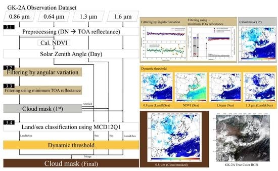
Owing to the high temporal resolution of the GK-2A, there is a large opportunity to obtain clear-sky reflectance even if there is an influx of clouds. In addition, variations in TOA reflectance due to cloud inflow and the occurrence of convective clouds can be identified. Since these advantages are useful for cloud masks, we developed a four-step cloud detection algorithm, as shown in Figure 3.
- Preprocessing;
- Filtering by angular variation;
- Filtering using minimum TOA reflectance;
- Dynamic threshold.
We primarily used 0.86 in the processes of filtering techniques and dynamic thresholds because 0.86 is widely used in various daytime cloud detection algorithms [13,16,37,38]. The other channels of 0.64, 1.38, and 1.6 were additionally used in the dynamic threshold section to improve the accuracy of the cloud mask. In case of 0.64 , we used this channel to calculate NDVI. All the imagery was resampled to 2 km using linear spline interpolation.
3.1. Preprocessing
The digital number (DN) of the GK-2A observation dataset was converted to TOA reflectance to facilitate identification of the data in each pixel and to minimize the effect of the solar zenith angle.
where denotes the TOA reflectance, are the pixel coordinates, is the wavelength, is the distance between Earth and Sun in astronomical units, are the gain and offset to convert DN to radiance, respectively, is the mean solar exoatmospheric irradiance, and is the solar zenith angle. can be calculated by integrating the solar spectral irradiance and the GK-2A spectral response function spectral response function (). The solar spectrum to derive solar spectral irradiance () is acquired from the National Renewable Energy Laboratory (NREL) webpage [39,40,41]. We used the synthetic Gueymard spectrum, which covers the spectral region from 0.4 to 1.7 in 1 steps and from 1.7 to 4 in 5 steps [40]. Because a difference in resolution between the solar spectrum and GK-2A exists, we used linear interpolation.
The values of 0.6, 0.8, 1.3, and 1.6 were calculated and are shown in Table 1.
3.2. Filtering Technique by Angular Variation
Reflectance represents the ratio of reflected radiance to the incident flux at a specific surface. Reflectance under clear-sky conditions is almost unchanged if the effect of the change in solar zenith angle is corrected and the effects of atmospheric components (scattering, absorption) are weak. As shown in Figure 4a, red and blue lines (dot) indicate the variation in reflectance observed under clear-sky conditions, and orange and cyan lines (square) indicate that clouds are approaching or flowing away from a specific pixel. When clouds approach a specific pixel, the reflectance of the pixel gradually increases. By using these characteristics, we propose the time-variant filtering technique by using angular variation to detect and mask cloud pixels. If there is a pixel located in a clear sky, change in reflectance over time should be approximately 45 degrees. However, since there are changes in reflectance due to variations in surface characteristics and atmospheric components that cause the scattering and absorption of radiance, the angle of reflectance varies within a certain range. As shown in Figure 4b, the upper figure shows the variation in angle in clear-sky reflectance, which is located in specific pixels of land and sea. The lower figure presents the change in angle caused by clouds. Regular angle variation can be checked in clear-sky observations through Figure 4b. The angle variation is more stable on land than on sea. Therefore, we set the threshold from 44° to 46° for both land and sea, and the range of thresholds was selected by finding the angular change in several pixels in clear-sky observations. The filtering technique is inspired by Graham’s scan algorithm, which is a method to find the convex hull of finite points on a plane.
where denotes an angle, is the acquisition time of imagery, is the time step, and we set 10 min as the time step.
3.3. Filtering Technique Using Minimum TOA Reflectance
If clouds continue to flow into the area, the filtering technique of angular variation cannot detect and mask the clouds. This is because high reflectance in the pixel is maintained. In other words, even though the pixel is located in clouds, the angle obtained as the time changes remains within 44° to 46° , similar to the clear-sky observation. Therefore, we solve this problem by using minimum TOA reflectance [42,43]. Specifically, we calculated the minimum TOA reflectance with a stacked dataset for seven days, and we calculated the difference between the target and minimum TOA reflectance. The cloud pixels were detected and masked by using a threshold calculated in advance. In this process, if only the minimum TOA reflectance was used to filter the clouds without using a threshold, the variation in reflectance due to the changes in surface characteristics and atmospheric components could not be considered. To prevent this problem, we used a threshold. To calculate the threshold, we need to fully separate cloud pixels from clear-sky observations in time series graphs. Therefore, we revised and used the cloth simulation filtering (CSF) method [44]. CSF was originally developed to find the shape of terrain, which is a digital surface model (DSM), by dropping a virtual cloth down on an inverted (upside-down) point cloud [44]. CSF consists of two steps: ‘displacement by gravity’ and ‘internal force’. Of these steps, we only used the displacement by gravity.
where denotes displacement by gravity, represents the minimum TOA reflectance, and it is calculated by accumulating all imagery for seven days before the target date; m is the mass of the particle, which is usually set to 1, and is the gravitational constant. We reverse the dataset by using and use Equation (4). The red dots shown in Figure 5 are the results of the calculated displacement by gravity. As shown in Figure 5a,c, if clouds which were not masked by filtering by angular variation exist, the difference from the minimum TOA reflectance (highest point, blue dot) is higher when using displacement by gravity than when using only the observed reflectance. Therefore, displacement by gravity used in this study amplifies the difference between the minimum and target TOA reflectance, as shown in Figure 5.
To calculate the threshold, we stacked the TOA reflectance dataset for 30 days in June 2020 and used the Otsu multilevel threshold method with three classes, as shown in Figure 6 [45,46].
where k denotes the clusters, indicates the cumulative probability, indicates the mean gray level for each cluster, indicates the mean intensity of the whole image, and denotes the between-class variance. The optimal threshold can be determined by maximizing the between-class variance [46]. Among the thresholds, the closest to the cloud pixel value of 4.237, as shown in Figure 6, was used.
3.4. Dynamic Threshold
Because of atmospheric blocking and the occurrence of stationary fronts due to the expansion of the North Pacific high, pixels where clouds are constantly maintained exist in the image. As shown in Figure 7a, the pixels with remained clouds that are not masked when using the proposed filtering techniques mentioned above appear to have higher TOA reflectance than other pixels. Since these cloud pixels are less distributed among the whole image, we set the threshold value through the Otsu multilevel threshold method [45,46], which is used in Section 3.3. The number of classes was set to 4, which was determined empirically. Additionally, to improve the accuracy of the proposed algorithm, the NIR and NDVI images applied with cloud mask, which was result of the proposed filtering techniques, were also used in this study with the Otsu method, as shown in Figure 7. Among the thresholds, the closest to the cloud pixel value was used. When a dynamic threshold was applied to the channels, we divided the land and sea areas by using annual International Geosphere-Biosphere Programme (IGBP) classification data of MCD12Q1 [47], which is the MODIS Terra and Aqua combined land cover product. After reprojection of MCD12Q1 data to Lambert Conic Conformal (LCC), only the data over the water bodies were used.
3.4.1. NDVI
The NDVI is a frequently used index that expresses the status of plant health. In particular, the NDVI has been useful in analyzing temporal changes in vegetation [45]. The range of the NDVI is from −1 to 1. If the pixel value approaches 0, there is a small difference between the observed radiances of the red and NIR channels. A pixel value near zero indicates sand, clouds, and rocks [48,49,50]. Therefore, if the NDVI is applied to land to classify cloud pixels, it is difficult to be used because the TOA reflectance of cloud is similar to that of the desert [51]. For this reason, only the NDVI in the sea was used in this study.
where and indicate the TOA reflectance of and , respectively, which are calculated by Equation (1).
3.4.2. Near-Infrared
We used 1.38 and 1.6 in the dynamic threshold part. The 1.38 (from 1.36 to 1.39 ) channel is located in strong atmospheric water absorption. It is observed by radiance mainly reflected by the troposphere because the upward radiance from the surface or the lower-middle atmosphere is blocked by water vapor in the upper atmosphere [52]. Therefore, 1.38 has been used for decades in MODIS to detect cirrus clouds even over polar regions where the atmosphere is extremely dry [13,23]. The threshold to detect thick cirrus clouds is set to 0.02 globally in MODIS and Landsat-8 cloud products [23]. In the case of the MODIS cloud product, separate thresholds are divided according to the existence of snow and confidence levels [12,23]. In this study, we set the initial global threshold to 0.02 and then adjust the threshold by applying the Otsu method because the use of the global threshold misses some thin cirrus clouds.
4. Results
As the solar radiance reaching Earth gradually increases from June to August, the North Pacific high shifts to the north, and low pressure occurs in East Asia [55]. On the other hand, dry air from the north acts as a kind of ‘invisible wall’ that blocks the movement of moist air, and as a result, a large amount of water vapor in the atmosphere falls as rain [55]. Therefore, in general, precipitation increases in southeastern China and Japan in mid-June, increases in South Korea in late June, and then moves north to North Korea [55]. In July 2020, the extreme values of average temperature, maximum temperature, and the number of heatwave days were updated in the Rep. of Korea. At the end of June, since the North Pacific high was located in the southeastern Rep. of Korea, the low pressure that developed in southern China approached, the southwest wind strengthened, and a large amount of water vapor was introduced.
As the North Pacific high is maintained until the first half of September, it shows a form of an atmospheric pressure pattern in summer, causing a temporary high temperature phenomenon [56]. In October, a migratory anticyclone develops in inland of China and moves eastward, generating clear and dry air [56]. Therefore, cirrus, cirrostratus, and cumulus clouds are primarily created. In case of October 2020, the seven typhoons were occurred in East Asia due to continuance of La Niña [57]. This is the unusual natural phenomena compared with the occurrence of three typhoon in October of normal year (1981 to 2010) [57]. Therefore, we select June and October 2020 as the date to compare and validate the proposed algorithm because various cloud types can be found.
We conducted a qualitative comparison and quantitative validation with GK-2A and LEO cloud products. For the qualitative comparison, the true color image and natural color image, which were made by using the RGB recipe of NMSC, were used [52]. For the quantitative validation, we used the confusion matrix as shown in Figure 8, and the precision, recall, accuracy (hit rate), false positive rate (FPR), and F1score were calculated to compare the proposed algorithm with LEO products. The precision and FPR are also referred to as the probability of detection (POD) and false alarm rate (FAR), respectively [15,58].
where true positive () means the number of pixels when validation data was cloud, and proposed algorithm was set to cloud. False positive () means the number of pixels when validation data was clear observation, and proposed algorithm was set to cloud. False negative () means the number of pixels when validation data was cloud, and proposed algorithm was set to clear observation. True negative () means the number of pixels when validation data was clear observation, and proposed algorithm was set to clear observation, as shown in Figure 8.
The precision indicates how accurate the masked cloud pixel from GK-2A is. In other words, it shows how many pixels that are actual clouds are included in the GK-2A cloud detection results. The recall indicates how well the cloud was found without dropping it. The accuracy is an indicator of how accurately the proposed algorithm detects clouds. The FPR is the probability of falsely rejecting the null hypothesis. The F1score calculated by the harmonic mean represents the difference between precision and recall. If the difference between the two values increases, the F1score increases, and if the difference between the two values decreases, the F1score decreases.
4.1. Qualitative Comparison
As a qualitative comparison of the proposed algorithm, the true color and natural color images, which are made by GK-2A images, are used. The true color RGB is designed close to the human eye and is made by using visible channels (0.47 , hybrid green, 0.64 ) applied with histogram equalization. Hybrid green is calculated by using and [52]. The natural color RGB is designed to distinguish ice from the water phase and is made by using visible channels (, ) and a NIR channel (1.6 ) applied with histogram equalization [52].
The only 3 dates of June 2020 were used as shown in Figure 9. The area colored grey in Figure 9c,i is removed by the restriction of the solar zenith angle. In the case of 1 June 2020 00 UTC, as shown in Figure 9a–c, the proposed algorithm can detect convective clouds occurring over the Shandong Peninsula (37.175° N, 121.297° E) of China and cirrus clouds over the Yellow Sea and East Sea of the Rep. of Korea, in addition to detecting the overall clouds. In the case of 08 June 2020 03 UTC, as shown in Figure 9d–f, the stationary front located at 20° N is well detected, and the cirrus clouds located on land (40° N, 90° E) are also well detected. As shown in Figure 9g–i, most of the clouds, including cirrus, were well detected. However, the cloud detection accuracy is decreased in the area where sunglint occurs (Figure 9c,f). When sunlight is reflected off the sea at the same angle as the satellite sensor detects the surface, sunglint occurs. Therefore, the area where sunglint occurs varies over time. Since the proposed algorithm is based on multitemporal images, error occurs due to phenomena that change with time, such as sunglint.
The only 3 dates of October 2020 were used as shown in Figure 10. In the case of 2 June 2020 01 UTC, as shown in Figure 10a–c, most of opaque clouds can be detected over land and sea. Especially, proposed algorithm can detect cirrus clouds over Jeju Island in Rep. of Korea (33.387° N, 126.556° E) and neighboring sea (Southern sea of Rep. of Korea). In case of 11 October 2020 04 UTC, as shown in Figure 10d–f, typhoon Chan-Hom and accompanying clouds are clearly detected in the sea located east (33.784° N, 139.786° E) of Tokyo, Japan. However, as compared with true color RGB in Figure 10d, misclassified results as clouds were found in Qinghai Province (35° N, 95° E), China. The reason why misclassified result was revealed is that dust storm was occurred and the effect of solar zenith angle in desert still remained.
4.2. Validation with the VIIRS Cloud Product
The VIIRS cloud product was collected for 60 days from 1 to 30 in June and October 2020 to validate the proposed algorithm. The VIIRS cloud product distinguishes between confident and probably clouds according to the threshold test. The VIIRS cloud mask sets three thresholds between high confidence cloudy and high confidence clear and uses these thresholds to determine the confidence flag [13]. According to the validation score of the VIIIRS cloud mask, the overall hit rate (%) was 88.4% in July 2007 and 89% in October 2007 [59].
In this study, confident and probably clouds were classified and validated with the proposed algorithm and GK-2A cloud mask. The GK-2A cloud mask was originally developed by NMSC and is available via webpage [60]. The GK-2A cloud mask also provides clouds as confident and probably by using threshold tests similar to the VIIRS cloud detection algorithm. Therefore, when only confident clouds in VIIRS products were used, only confident clouds in GK-2A cloud masks were used, and the same was applied when using probably clouds.
The result of validation with the VIIRS cloud product is shown in Table 2, and when VIIRS with confident and probably clouds was used, the accuracy of both the multitemporal and spectral-based algorithms was higher. In the case of the spectral-based algorithm, the precision, recall, accuracy, and F1score significantly increased. However, when compared with the proposed multitemporal algorithm, the degree of agreement with the VIIRS cloud product is significantly different as difference of the accuracy is 0.15, and the F1score is 0.1 as mean value between June and October. In the case of the recall value in the comparison between the proposed algorithm and VIIRS with confident and probably clouds, as shown in Table 2, the result was close to 1. The VIIRS cloud data and the proposed GK-2A cloud detection algorithm are almost identical. In addition, since the F1score of the proposed algorithm represents 0.92 (June and October), the proposed algorithm has good performance in detecting clouds.
4.3. Validation with the CALIPSO Cloud Product
In this section, we compare the CALIPSO cloud product and proposed algorithm, as shown in Table 3. The CALIPSO cloud product was collected for 60 days from 1 to 30 June and October 2020 to validate the proposed algorithm. In the case of the GK-2A (NMSC) cloud mask, when the dataset used both confident and probably clouds, the accuracy was slightly higher in Section 4.2. Therefore, we used both confident and probably clouds in this section. As a result of validation with CALIPSO, the proposed algorithm showed a high accuracy of 0.92, which is mean value (Table 3). The all of precision, recall, and F1score also showed high values of about 0.9 or higher (Table 3). Compared to GK-2A (NMSC) cloud detection, the proposed algorithm is superior based on the overall indexes. Therefore, these results indicated that the proposed algorithm detects most of the clouds with good performance.
Additionally, we conducted an accuracy assessment according to cloud types, which is provided from ‘Feature_Classification_Flags’ of the CALIPSO cloud product. Eight cloud types (feature subtype) were classified in the CALIPSO cloud dataset. We evaluated whether the proposed algorithm detects each cloud type well, as shown in Figure 11. For validation by cloud types, we used only the recall because the pixels, which are located in clear-sky conditions or classified by aerosols, were set to not-a-number (NaN) values in the cloud product. As the results of validation by cloud types, recall values of 0.96 or higher are shown in Figure 11. Among the eight cloud types, low (broken cumulus) and altocumulus (transparent) had the lowest recall values of 0.96. Since the two types of clouds are smaller than the other clouds, the proposed algorithm classified a few pixels with these two types of clouds as clear sky. However, since the overall result had a very high score, there seems to be no loss of accuracy depending on cloud types.
5. Discussions
The proposed algorithm has four steps to detect clouds. Each step must be in harmony with the others to derive the results shown in Table 2 and Table 3. The harmony of each step can be checked with a simple accuracy test for each step. We divided algorithms (1) with all steps, (2) that used only filtering techniques by using angular variation and minimum TOA reflectance, and (3) that used only the dynamic threshold for each GK-2A channel. The test dataset to check the accuracy of each step is set to 30 days (1 to 30 June 2020) of collocated images between GK-2A and VIIRS, as shown in Table 4. When only filtering techniques were used, the accuracy and F1score decreased by approximately 0.05 and 0.03, respectively. Additionally, when using only the dynamic threshold for GK-2A NIR and NDVI images, the accuracy was decreased by approximately 0.4. These results mean that all the steps are operating harmoniously. As mentioned above, if only filtering techniques were used, abnormal TOA reflectance was revealed due to the existence of clouds on stacking days. In addition, if images not to be applied with filtering methods were used in the dynamic threshold step, the threshold values in each channel used in this study were irregular. This is because the Otsu threshold method found the point of inflection in each image histogram. In other words, when an image is applied with filtering techniques, the rest of the cloud can be easily found because there is a gap between the surface and the remaining cloud.
Regarding thresholds used in filtering techniques of proposed algorithm, it is effective even if the thresholds were applied to images of other seasons. In other words, the thresholds were calculated from images acquired for one month of June 2020. When the thresholds were applied in other images acquired in October 2020, the satisfactory results were obtained as shown in Table 2 and Table 3. It can be shown as an advantage of proposed algorithm, because the problems that arise when applying this algorithm in other seasons can be flexibly captured through the fusion of filtering techniques and dynamic threshold.
Although the accuracy of the proposed algorithm of the GK-2A cloud mask was found to be reliable according to statistical values, this algorithm involves some issues due to sunglint and desert areas. In case of sunglint, Figure 9c,f show the areas misclassified as clouds, although they are under clear-sky conditions. As mentioned above, the problem was a change in sunglint area. When the sunglint area moved from east to west over the daytime, the reflectance on the sea fluctuated. Since it is caused by angular variation in specific pixels, error in the sunglint area occurs. In case of desert, some area was misclassified as clouds because of dust storm and the effect of solar zenith angle in desert, as shown in Figure 10f. Therefore, additional approaches of GK-2A multitemporal cloud detection should be considered.
6. Summary and Conclusions
We propose a cloud detection algorithm with GK-2A multitemporal and multispectral images during the daytime. The steps are to (1) find and mask the cloud pixels if TOA reflectance changes greatly as time changes; (2) find and mask the remaining cloud pixels by using the difference with minimum TOA reflectance; and (3) find and mask the remaining cloud pixels by additionally using NIR and NDVI images applied with a dynamic threshold. All the steps in this study operate in harmony. We evaluated the reason why three steps are needed to detect clouds. In addition, we evaluated whether the proposed algorithm is very well suited to classify clouds, as validated with frequently used CALIPSO and VIIRS cloud products. The validation result indicates that the proposed cloud detection algorithm detects most of the clouds with good performance. Although the cloud detection algorithm obtains satisfactory results, the misclassification occurs in sunglint and desert areas. Because the proposed cloud detection algorithm is based on multitemporal data, the variance in TOA reflectance affected by sunglint and the remained effect of solar zenith angle in desert area cause misclassification. In the future, we will try to develop an additional algorithm to solve the misclassification.
Author Contributions
Conceptualization, S.L. and J.C.; data curation, S.L.; funding acquisition, J.C.; investigation, S.L. and J.C.; methodology, S.L. and J.C.; software, S.L.; visualization, S.L.; writing—original draft, S.L.; and writing—review and editing, J.C. All authors have read and agreed to the published version of the manuscript.
Funding
This study was funded by the Basic Science Research Program through the National Research Foundation of Korea (NRF), which is funded by the Ministry of Education (NRF-2020R1I1A3A04037483).
Informed Consent Statement
Not applicable.
Data Availability Statement
The GK-2A imagery used in this study are available on request from the NMSC webpage (http://datasvc.nmsc.kma.go.kr/datasvc/html/main/main.do?lang=en) (accessed on 12 August 2021).
Acknowledgments
We would like to greatly appreciate the three reviewers and the editors for their valuable comments.
Conflicts of Interest
The authors declare no conflict of interest.
References
- Mahajan, S.; Ftaniya, B. Cloud detection methodologies: Variants and development—A review. Complex Intell. Syst. 2020, 6, 251–261. [Google Scholar] [CrossRef] [Green Version]
- Yin, J.; Porporato, A. Diurnal cloud cycle biases in climate models. Nat. Commun. 2017, 8, 2269. [Google Scholar] [CrossRef] [PubMed] [Green Version]
- Norris, J.R.; Allen, R.J.; Evan, A.T.; Zelinka, M.D.; O’Dell, C.W.; Klein, S.A. Evidence for climate change in the satellite cloud record. Nature 2016, 536, 72–75. [Google Scholar] [CrossRef] [PubMed] [Green Version]
- GCOS. Available online: https://gcos.wmo.int/en/essential-climate-variables/clouds (accessed on 15 April 2021).
- Marais, I.Z.; Preez, J.A.; Steyn, W.H. An optimal image transform for threshold-based cloud detection using heteroscedastic discriminant analysis. Int. J. Remote Sens. 2011, 32, 1713–1729. [Google Scholar] [CrossRef]
- Gutman, G.G. Satellite daytime image classification for global studies of Earth’s surface parameters from polar orbiters. Int. J. Remote Sens. 1992, 13, 1–17. [Google Scholar] [CrossRef]
- Chen, P.; Srinivasan, R.; Fedosejevs, G. An automated cloud detection method for daily NOAA 16 advanced very high resolution radiometer data over Texas and Mexico. J. Geophys. Res. Atmos. 2003, 108, 4742. [Google Scholar] [CrossRef]
- Du, W.; Qin, Z.; Fan, J.; Gao, M.; Wang, F.; Abbasi, B. An efficient approach to remove thick cloud in VNIR bands of multi-temporal remote sensing images. Remote Sens. 2019, 11, 1284. [Google Scholar] [CrossRef] [Green Version]
- Sun, L.; Wei, J.; Wang, J.; Mi, X.; Guo, Y.; Lv, Y.; Yang, Y.; Gan, P.; Zhou, X.; Jia, C.; et al. A Universal dynamic threshold cloud detection algorithm (UDTCDA) supported by a prior surface reflectance database. J. Geophys. Res. Atmos. 2016, 121, 7172–7196. [Google Scholar] [CrossRef]
- Drönner, J.; Korfhage, N.; Egli, S.; Mühling, M.; Thies, B.; Bendix, J.; Freisleben, B.; Seeger, B. Fast cloud segmentation using convolutional neural networks. Remote Sens. 2018, 10, 1782. [Google Scholar] [CrossRef] [Green Version]
- Chen, Y.; Fan, R.; Bilal, M.; Yang, X.; Wang, J.; Li, W. Multilevel cloud detection for high-resolution remote sensing imagery using multiple convolutional neural networks. ISPRS Int. J. Geoinf. 2018, 7, 181. [Google Scholar] [CrossRef] [Green Version]
- Frey, R.A.; Ackerman, S.A.; Liu, Y.; Strabala, K.I.; Zhang, H.; Key, J.R.; Wang, X. Cloud detection with MODIS. Part I: Improvements in the MODIS cloud mask for collection 5. J. Atmos. Ocean. Technol. 2008, 25, 1057–1072. [Google Scholar] [CrossRef]
- Ackerman, S.A.; Strabala, K.I.; Menzel, S.W.; Frey, R.A.; Moeller, C.C.; Gumley, L.E. Discriminating clear sky from clouds with MODIS. J. Geophys. Res. 1998, 103, 32141–32157. [Google Scholar] [CrossRef]
- Dybbroe, A.; Karlsson, K.G.; Thoss, A. NWCSAF AVHRR cloud detection and analysis using dynamic thresholds and radiative transfer modeling. Part II: Tuning and validation. J. Appl. Meteorol. Climatol. 2005, 44, 55–71. [Google Scholar] [CrossRef]
- Jang, J.C.; Lee, S.; Sohn, E.H.; Noh, Y.J.; Miller, S.D. Combined dust detection algorithm for Asian dust events over East Asia using GK2A/AMI: A case study in October 2019. Asia-Pacific J. Atmos. Sci. 2021, 1–20. [Google Scholar] [CrossRef]
- Kim, H.; Lee, B. GK-2A AMI Algorithm Theoretical Basis Document: Cloud Mask; National Meteorological Satellite Center: Jincheon-gun, Korea, 2019; pp. 1–37. [Google Scholar]
- Lubin, D.; Morrow, E. Evaluation of an AVHRR cloud detection and classification method over the central Arctic ocean. J. Appl. Meteorol. Climatol. 1998, 37, 166–183. [Google Scholar] [CrossRef]
- Liu, Y.; Key, J.R.; Frey, R.A.; Ackerman, S.A.; Menzel, W.P. Nighttime polar cloud detection with MODIS. Remote Sens. Environ. 2004, 92, 181–194. [Google Scholar] [CrossRef]
- Yeom, J.M.; Roujean, J.L.; Han, K.S.; Lee, K.S.; Kim, H.W. Thin cloud detection over land using background surface reflectance based on the BRDF model applied to geostationary ocean color imager (GOCI) satellite data sets. Remote Sens. Environ. 2020, 239, 111610. [Google Scholar] [CrossRef]
- Stöckli, R.; Bojanowski, J.S.; John, V.O.; Duguay-Tetzlaff, A.; Bourgeois, Q.; Schulz, J.; Hollmann, R. Cloud detection with historical geostationary satellite sensors for climate applications. Remote Sens. 2019, 11, 1052. [Google Scholar] [CrossRef] [Green Version]
- Zhu, Z.; Woodcock, C.E. Automated cloud, cloud shadow, and snow detection in multitemporal landsat data: An algorithm designed specifically for monitoring land cover change. Remote Sens. Environ. 2014, 152, 217–234. [Google Scholar] [CrossRef]
- Zhu, Z.; Wang, S.; Woodcock, C.E. Improvement and expansion of the Fmask algorithm: Cloud, cloud shadow, and snow detection for landsats 4–7, 8, and Sentinel 2 images. Remote Sens. Environ. 2015, 159, 269–277. [Google Scholar] [CrossRef]
- Qiu, S.; Zhu, Z.; Woodcock, C.E. Cirrus clouds that adversely affect landsat 8 images: What are they and how to detect them? Remote Sens. Environ. 2020, 246, 1–17. [Google Scholar] [CrossRef]
- Belgiu, M.; Dragut, L. Random forest in remote sensing: A review of applications and future directions. ISPRS J. Photogramm. Remote Sens. 2016, 114, 24–31. [Google Scholar] [CrossRef]
- Sim, S.; Im, J.; Park, S.; Park, H.; Ahn, M.H.; Chan, P. Icing detection over East Asia from geostationary satellite data using machine learning approaches. Remote Sens. 2018, 10, 631. [Google Scholar] [CrossRef] [Green Version]
- Han, D.; Lee, J.; Im, J.; Sim, S.; Lee, S.; Han, H. A novel framework of detecting convective initiation combining automated sampling, machine learning, and repeated model tuning from geostationary satellite data. Remote Sens. 2019, 11, 1454. [Google Scholar] [CrossRef] [Green Version]
- Taravat, A.; Proud, S.; Peronaci, S.; Del Frate, F.; Oppelt, N. Multilayer perceptron neural networks model for meteosat second generation SEVIRI daytime cloud masking. Remote Sens. 2015, 7, 1529–1539. [Google Scholar] [CrossRef] [Green Version]
- Xie, F.; Shi, M.; Shi, Z. Multilevel cloud detection in remote sensing images based on deep learning. IEEE J. Sel. Top. Appl. Earth Obs. Remote Sens. 2017, 10, 3631–3640. [Google Scholar] [CrossRef]
- Yang, J.; Guo, J.; Yue, H.; Liu, Z.; Hu, H.; Li, K. CDnet: CNN-based cloud detection for remote sensing imagery. IEEE Trans. Geosci. Remote Sens. 2019, 57, 6195–6211. [Google Scholar] [CrossRef]
- National Meteorological Satellite Center (NMSC). Available online: http://datasvc.nmsc.kma.go.kr/datasvc/html/base/cmm/selectPage.do?page=static.openApi2 (accessed on 12 August 2021).
- Cao, C.; Xiong, J.; Blonki, S.; Liu, Q.; Uprety, S.; Shao, X.; Bai, Y.; Weng, F. Suomi NPP VIIRS sensor data record verification, validation, and long-term performance monitoring. J. Geophys. Res. Atmos. 2013, 118, 11664–11678. [Google Scholar] [CrossRef]
- EARTHDATA. Available online: https://earthdata.nasa.gov/ (accessed on 12 August 2021).
- Kopp, T.J.; Thomas, W.; Heidinger, A.K.; Botambekov, D.; Frey, R.A.; Hutchison, K.D.; Iisager, B.D.; Brueske, K.; Reed, B. The VIIRS cloud mask: Progress in the first year of S-NPP toward a common cloud detection scheme. J. Geophys. Res. Atmos. 2014, 119, 2441–2456. [Google Scholar] [CrossRef]
- Stephens, G.L.; Vane, D.G.; Boain, R.J.; Mace, G.G.; Sasse, K.; Wang, J.; Illingworth, A.J.; Oconnor, E.J.; Rossow, W.B.; Durden, S.L.; et al. The CLOUDSAT mission and the A-TRAIN: A new dimension of space-based observations of clouds and precipitation. Bull. Amer. Meteor. Soc. 2002, 83, 1771–1790. [Google Scholar] [CrossRef] [Green Version]
- Winder, D.M.; Vaughan, M.A.; Omar, A.; Hu, Y.; Powell, K.A.; Liu, Z.; Hunt, W.H.; Young, S.A. Overview of the CALIPSO mission and CALIOP data processing algorithms. J. Atmos. Ocean. Technol. 2009, 26, 2310–2323. [Google Scholar] [CrossRef]
- Lee, K.H. 3-D perspectives of atmospheric aerosol optical properties over Northeast Asia using LIDAR on-board the CALIPSO satellite. Korean J. Remote Sens. 2014, 30, 559–570. [Google Scholar] [CrossRef]
- Hocking, J.; Francis, P.N.; Saunders, R. Cloud detection in meteosat second generation imagery at the met office. Meteorol. Appl. 2011, 18, 307–323. [Google Scholar] [CrossRef]
- Sun, L.; Mi, X.; Wei, J.; Wang, J.; Tian, X.; Yu, H.; Gan, P. A cloud detection algorithm-generating method for remote sensing data at visible to short-wave infrared wavelengths. ISPRS J. Photogramm. Remote Sens. 2017, 124, 70–88. [Google Scholar] [CrossRef]
- National Renewable Energy Laboratory (NREL). Available online: https://www.nrel.gov/grid/solar-resource/spectra.html (accessed on 12 August 2021).
- Gueymard, C.A. The sun’s total and spectral irradiance for solar energy applications and solar radiation models. Sol. Energy 2004, 76, 423–453. [Google Scholar] [CrossRef]
- Trishchenko, A.P. Solar irradiance and effective brightness temperature for SWIR channels of AVHRR/NOAA and GOES imagers. J. Atmos. Ocean. Technol. 2005, 23, 198–210. [Google Scholar] [CrossRef]
- Shen, H.; Li, H.; Qian, Y.; Zhang, L.; Yuan, Q. An effective thin cloud removal procedure for visible remote sensing images. ISPRS J. Photogramm. Remote Sens. 2014, 96, 224–235. [Google Scholar] [CrossRef]
- Chen, B.; Huang, B.; Chen, L.; Xu, B. Spatially and temporal weighted regression: A novel method to produce continuous cloud-free Landsat imagery. IEEE Trans. Geosci. Remote Sens. 2017, 55, 27–37. [Google Scholar] [CrossRef]
- Zhang, W.; Qi, J.; Wan, P.; Wang, H.; Xie, D.; Wang, X.; Yan, G. An easy-to-use airborne LiDAR data filtering method based on cloth simulation. Remote Sens. 2016, 8, 501. [Google Scholar] [CrossRef]
- Liao, P.S.; Chen, T.S.; Chung, P.C. A fast algorithm for multilevel thresholding. J. Inf. Sci. Eng. 2001, 17, 713–727. [Google Scholar]
- Huang, D.Y.; Lin, T.W.; Hu, W.C. Automatic multilevel thresholding based on two-stage OTSU’s method with cluster determination by valley estimation. Int. J. Innov. Comput. Inf. Control. 2011, 7, 5631–5644. [Google Scholar]
- Liang, D.; Zuo, Y.; Huang, L.; Zhao, J.; Teng, L.; Yang, F. Evaluation of consistency of MODIS land cover product (MCD12Q1) based on chines 30 m GlobLand30 datasets: A case study in anhui province, China. ISPRS Int. J. Geo-Inf. 2015, 4, 2519–2541. [Google Scholar] [CrossRef] [Green Version]
- Schreyers, L.; Emmerik, T.; Biermann, L.; Lay, Y.L. Spotting green tides over Brittany from space: Three decades of monitoring with landsat imagery. Remote Sens. 2021, 13, 1408. [Google Scholar] [CrossRef]
- Xiong, Q.; Wang, Y.; Liu, D.; Ye, S.; Du, Z.; Liu, W.; Huang, J.; Su, W.; Zhu, D.; Yao, X.; et al. A cloud detection approach based on hybrid multispectral features with dynamic thresholds for GF-1 remote sensing images. Remote Sens. 2020, 12, 450. [Google Scholar] [CrossRef] [Green Version]
- Ya’acob, N.; Azize, A.B.M.; Mahmon, N.A.; Yusof, A.L.; Azmi, N.F.; Mustafa, N. Temporal forest change detection and forest health assessment using remote sensing. IOP Conf. Ser. Earth Environ. Sci. 2014, 19, 12017. [Google Scholar] [CrossRef] [Green Version]
- Escadafal, R. Remote sensing drylands: When soils come into the picture. Ci. Tróp. Recif. 2017, 41, 33–50. [Google Scholar]
- National Meteorological Satellite Center (NMSC). Available online: http://wiki.nmsc.kma.go.kr/doku.php?id=start (accessed on 28 April 2021).
- Dozier, J. Spectral signature of alpine snow cover from LANDSAT Thematic Mapper. Remote Sens. Environ. 1989, 28, 9–22. [Google Scholar] [CrossRef]
- Heidinger, A.K.; Frey, R.; Pavolonis, M. Relative merits of the 1.6 and 3.75 μm channels of the AVHRR/3 for cloud detection. Can. J. Remote Sens. 2014, 30, 182–194. [Google Scholar] [CrossRef]
- Institute for Basic Science (IBS). Available online: https://www.ibs.re.kr/cop/bbs/BBSMSTR_000000000735/selectBoardArticle.do?nttId=19049 (accessed on 28 April 2021).
- Korea Meteorological Administration (KMA). Available online: https://m.blog.naver.com/PostView.naver?blogId=kma_131&logNo=222145676520&referrerCode=0&searchKeyword=10%EC%9B%94 (accessed on 1 July 2021).
- Korea Meteorological Administration (KMA). Available online: https://www.korea.kr/news/policyBriefingView.do?newsId=148605200 (accessed on 1 July 2021).
- Frey, R.A.; Ackerman, S.A.; Holz, R.E.; Dutcher, S.; Griffith, Z. The continuity MODIS-VIIRS cloud mask. Remote Sens. 2020, 12, 3334. [Google Scholar] [CrossRef]
- Frey, R.A.; Heidinger, A.K.; Hutchison, K.D.; Dutcher, S. VIIRS cloud mask validation exercises. AGU Fall Meeting Abstracts, San Francisco, CA, USA, 5–9 December; 2011. 0265. [Google Scholar]
- National Meteorological Satellite Center (NMSC). Available online: https://nmsc.kma.go.kr/homepage/html/satellite/viewer/selectSatViewer.do?dataType=operSat# (accessed on 12 August 2021).
Figure 1.
Study area of East Asia.

Figure 2.
Example of comparison and validation dataset: (a) GK-2A cloud mask acquired from 15 June 2020 03:00 UTC, (b) CALIPSO cloud product acquired from 15 June 2020 05:40 UTC. The red line in the image denotes path of CALIPSO data in specific time range, and (c) VIIRS cloud mask acquired from 15 June 2020 06:50 UTC.

Figure 3.
Flowchart of GK-2A multitemporal cloud detection algorithm.

Figure 4.
Variations in TOA reflectance of 0.86 and the angle of cloud/clear-sky pixels (6 June 2020 and 8 June 2020) in specific locations (land: 36.76° N/127.48° E, sea: 39.01° N/128.58° E): (a) TOA reflectance and (b) angle in degrees over UTC time.
Figure 4.
Variations in TOA reflectance of 0.86 and the angle of cloud/clear-sky pixels (6 June 2020 and 8 June 2020) in specific locations (land: 36.76° N/127.48° E, sea: 39.01° N/128.58° E): (a) TOA reflectance and (b) angle in degrees over UTC time.

Figure 5.
Graph of filtering process using minimum TOA reflectance. The TOA reflectance in the imagery were converted to . The bar graph indicates the difference between blue and red dots, the blue point indicates the minimum TOA reflectance, the red point indicates the value calculated by Equation (4), and the black point indicates the real TOA reflectance. Comparison between target (Displacement by gravity) and minimum TOA reflectance (Highest point) on land (36.76° N/127.48° E) (a) 7 June 2020 and (b) 8 June 2020; (c,d) are comparison on sea (39.01° N/128.58° E) (c) 10 June 2020 and (d) 8 June 2020; (a,c) mean that the values change when clouds flow into or disappear the specific pixel, and (b,d) mean clear-sky.

Figure 6.
Kernel Density Estimation (KDE) of the difference between the target and minimum TOA reflectance. The red lines indicate the threshold values calculated from the Otsu multi-threshold method. We used the threshold on the right side. The number of data points was 65,609,628, which were stacked over 30 days in land and sea areas.

Figure 7.
Results from applying the dynamic threshold. The imagery was captured on 15 June 2020 at 03:00 UTC: (a) the TOA reflectance of 0.8 applied by filtering techniques using angular variation and minimum TOA reflectance; (b) the result of applying the dynamic threshold by classifying land and sea in (a); (c) the NDVI in the sea with the dynamic threshold; (d) the TOA reflectance of 1.6 in the sea with the dynamic threshold; and (e) the TOA reflectance of 1.3 with the dynamic threshold. Originally, an initial threshold of 0.02 is applied. Therefore, the maximum of the color bar is set to 0.02. (f) The result from applying the filtering methods and dynamic threshold. It is produced by applying the results of (c–e) to (b).


Figure 8.
Confusion matrix.

Figure 9.
Qualitative comparison with GK-2A-based true color and natural color RGB in June 2020. Images are listed in the order of the true color, natural color, and proposed cloud mask, and each row is separated by date: (a–c) are at 00 UTC on 1 June 2020; (d–f) are at 03 UTC on 8 June 2020; and (g–i) are at 08 UTC on 24 June 2020.

Figure 10.
Qualitative comparison with GK-2A-based true color and natural color RGB in October 2020. Images are listed in the order of the true color, natural color, and proposed cloud mask, and each row is separated by date: (a–c) are examples at 01 UTC on 2 October 2020; (d–f) are at 04 UTC on 11 October 2020; and (g–i) are at 07 UTC on 26 October 2020.

Figure 11.
Comparison of recall value between GK-2A (Multitemporal) and CALIPSO cloud product according to cloud types.
Figure 11.
Comparison of recall value between GK-2A (Multitemporal) and CALIPSO cloud product according to cloud types.


Table 1.
Mean solar exoatmospheric irradiance from visible to NIR channels of GK-2A.
| Band | 0.64 μm | 0.86 μm | 1.38 μm | 1.6 μm |
|---|---|---|---|---|
| 1638.95 | 977.48 | 360.87 | 246.16 |
Table 2.
Quantitative validation results between GK-2A and VIIRS cloud mask products.
| Precision | Recall | Accuracy | FPR | F1score | |||
|---|---|---|---|---|---|---|---|
| VIIRS withConfident Clouds | June | GK-2A (Multitemporal) | 0.905 | 0.981 | 0.912 | 0.249 | 0.939 |
| GK-2A (NMSC) | 0.758 | 0.731 | 0.631 | 0.644 | 0.744 | ||
| October | GK-2A (Multitemporal) | 0.832 | 0.982 | 0.856 | 0.395 | 0.901 | |
| GK-2A (NMSC) | 0.622 | 0.741 | 0.520 | 0.945 | 0.677 | ||
| VIIRS withConfident and Probably Clouds | June | GK-2A (Multitemporal) | 0.911 | 0.977 | 0.912 | 0.281 | 0.943 |
| GK-2A (NMSC) | 0.807 | 0.913 | 0.772 | 0.645 | 0.857 | ||
| October | GK-2A (Multitemporal) | 0.842 | 0.972 | 0.856 | 0.395 | 0.902 | |
| GK-2A (NMSC) | 0.712 | 0.911 | 0.695 | 0.740 | 0.799 | ||
Table 3.
Quantitative validation results with CALIPSO cloud products.
| Number | Precision | Recall | Accuracy | FPR | F1score | |||
|---|---|---|---|---|---|---|---|---|
| CALIPSO Cloud | June | GK-2A (Multitemporal) | 199,807 | 0.891 | 0.982 | 0.902 | 0.284 | 0.934 |
| GK-2A (NMSC) | 210,415 | 0.784 | 0.935 | 0.775 | 0.601 | 0.853 | ||
| October | GK-2A (Multitemporal) | 190,382 | 0.911 | 0.989 | 0.930 | 0.184 | 0.949 | |
| GK-2A (NMSC) | 191,877 | 0.687 | 0.933 | 0.691 | 0.713 | 0.791 | ||
Table 4.
Accuracy test for each step of the GK-2A multitemporal cloud detection algorithm.
| Precision | Recall | Accuracy | FPR | F1score | ||
|---|---|---|---|---|---|---|
| GK-2A (Multitemporal) | 1 (Overall Steps) | 0.911 | 0.977 | 0.912 | 0.281 | 0.943 |
| 2 (Using only filtering techniques) | 0.881 | 0.949 | 0.866 | 0.379 | 0.914 | |
| 3 (Using only the dynamic threshold) | 0.711 | 0.652 | 0.542 | 0.783 | 0.681 | |
Publisher’s Note: MDPI stays neutral with regard to jurisdictional claims in published maps and institutional affiliations. |
© 2021 by the authors. Licensee MDPI, Basel, Switzerland. This article is an open access article distributed under the terms and conditions of the Creative Commons Attribution (CC BY) license (https://creativecommons.org/licenses/by/4.0/).
Share and Cite
MDPI and ACS Style
Lee, S.; Choi, J. Daytime Cloud Detection Algorithm Based on a Multitemporal Dataset for GK-2A Imagery. Remote Sens. 2021, 13, 3215. https://doi.org/10.3390/rs13163215
AMA Style
Lee S, Choi J. Daytime Cloud Detection Algorithm Based on a Multitemporal Dataset for GK-2A Imagery. Remote Sensing. 2021; 13(16):3215. https://doi.org/10.3390/rs13163215
Chicago/Turabian StyleLee, Soobong, and Jaewan Choi. 2021. "Daytime Cloud Detection Algorithm Based on a Multitemporal Dataset for GK-2A Imagery" Remote Sensing 13, no. 16: 3215. https://doi.org/10.3390/rs13163215
Note that from the first issue of 2016, this journal uses article numbers instead of page numbers. See further details here.