
Comparative Analysis of Variations and Patterns between Surface Urban Heat Island Intensity and Frequency across 305 Chinese Cities


State Key Laboratory of Remote Sensing Science, Faculty of Geographical Science, Beijing Normal University, Beijing 100875, China
*
Author to whom correspondence should be addressed.
Remote Sens. 2021, 13(17), 3505; https://doi.org/10.3390/rs13173505
Submission received: 9 August 2021
/
Revised: 29 August 2021
/
Accepted: 1 September 2021
/
Published: 3 September 2021
(This article belongs to the Special Issue Thermal and Optical Remote Sensing: Evaluating Urban Green Spaces and Urban Heat Islands in a Changing Climate)
Abstract
:Urban heat island (UHI), referring to higher temperatures in urban extents than its surrounding rural regions, is widely reported in terms of negative effects to both the ecological environment and human health. To propose effective mitigation measurements, spatiotemporal variations and control machines of surface UHI (SUHI) have been widely investigated, in particular based on the indicator of SUHI intensity (SUHII). However, studies on SUHI frequency (SUHIF), an important temporal indicator, are challenged by a large number of missing data in daily land surface temperature (LST). Whether there is any city with strong SUHII and low SUHIF remains unclear. Thanks to the publication of daily seamless all-weather LST, this paper is proposed to investigate spatiotemporal variations of SUHIF, to compare SUHII and SUHIF, to conduct a pattern classification, and to further explore their driving factors across 305 Chinese cities. Four main findings are summarized below: (1) SUHIF is found to be higher in the south during the day, while it is higher in the north at night. Cities within the latitude from 20° N and 40° N indicate strong intensity and high frequency at day. Climate zone-based variations of SUHII and SUHIF are different, in particular at nighttime. (2) SUHIF are observed in great diurnal and seasonal variations. Summer daytime with 3.01 K of SUHII and 80 of SUHIF, possibly coupling with heat waves, increases the risk of heat-related diseases. (3) K-means clustering is employed to conduct pattern classification of the selected cities. SUHIF is found possibly to be consistent to its SUHII in the same city, while they provide quantitative and temporal characters respectively. (4) Controls for SUHIF and SUHII are found in significant variations among temporal scales and different patterns. This paper first conducts a comparison between SUHII and SUHIF, and provides pattern classification for further research and practice on mitigation measurements.
1. Introduction
Over half of the world’s population have aggregated in urban areas [1], in particular with the rapid development of urbanization in recent years. Urbanization brings not only demographic and socioeconomic advancement, but also some urban environmental issues. The transformation, from natural surface to impervious areas, introduces evident perturbations to the Earth’s energy balance [2]. These perturbations can possibly be attributed to low albedo and high thermal capacity of impervious areas compared to evaporative vegetated cover [3,4]. Coupling with a mass of anthropogenic heat from rapid urbanization, urban heat island (UHI), with a higher temperature in urban extents than their surrounding areas, are reported in a large number of cities throughout the world [5,6,7,8,9,10,11,12,13,14,15,16]. The UHI is reported to be closely associated with a wide range of environmental issues, including air pollution [17], biodiversity reduction [18], and increased energy consumption [19,20]. Moreover, The UHI poses a potential threat to resident comfort and even human health, with increasing heat-related mortality [21,22], especially when heat waves strike simultaneously [23]. Thus, to propose effective mitigation measurements in future urban planning, extensive exploration of the variations and controls of UHI is necessary.
According to the way and height of observation, the UHI is generally grouped into two major categories: namely atmospheric (AUHI) and surface UHI (SUHI) [24,25]. The AUHI includes canopy and boundary UHI [5], which are detected by ground-based and high-altitude equipment, respectively. The sparse distribution and expensive installation of these observation measurements pose great challenges to AUHI studies, especially on a large scale. On the contrary, the SUHI takes advantage of thermal remote sensing with the capability of large-scale periodic observations [26]. Therefore, SUHI is reported as the main part of the UHI research from local to global scales [5].
Since Rao [27] first employed satellite-based data in the study of SUHI, a large number of SUHI studies have been published. Voogt and Oke [25] conducted a literature review on the application of thermal remote sensing in urban climates, and demonstrated their advantages in UHI studies. Streutker [28] explored the growth of SUHI in Houston, Texas from 1989 to 1999 based on an Advanced Very High Resolution Radiometer (AVHRR). Weng et al. [29] reported that interactions between land surface temperature (LST) and vegetation largely contribute to the spatial patterns of UHI, based on Landsat ETM+ thermal observation. Weng et al. [30] summarized the studies of urban climates based on remotely sensed thermal infrared (TIR) and pointed out that less attention has been paid to the estimation of UHI parameters. Imhoff et al. [7] analyzed the relationship between impervious surface area (ISA) and LST, and found great effects from the ecological context on the amplitude of SUHII during the summer daytime. Schwarz et al. [31] reported a large discrepancy and a low correlation among eleven different SUHI indicators, and suggested a combination of several indicators for comprehensive SUHI studies. Peng et al. [6] investigated SUHI across 419 global big cities and reported different driving mechanisms between daytime and nighttime. Quan et al. [32] employed the Gaussian volume model to explore the trajectory of SUHI in Beijing, and found temporal variations of the UHI centroid. Zhao et al. [33] reported that the efficiency of thermal convection make a strong contribution to the geographic variations of daytime UHI, and proposed albedo managements as promising mitigation measurements on a large scale. Zhou et al. [34] analyzed spatial–temporal patterns of SUHI across 32 major cities in China, and found that vegetation and anthropogenic heat were closely related to the SUHI during summer daytime. Lai et al. [35] proposed a four-parameter diurnal temperature cycle (DTC) model, and characterized 354 Chinese cities into five typical temporal patterns. Manoli et al. [36] introduced a coarse-grained model based on population and precipitation, and reported their strong contribution to magnitude of SUHI.
Taking advantage of remote sensing, SUHI intensity (SUHII) has been widely investigated. Despite considerable applications of satellite-based TIR data, TIR measurements are largely limited by their low tolerance to cloud cover [37,38,39,40,41], resulting in over half of the missing data [42]. Since there is a hard availability of daily seamless LST directly from the TIR products, the spatial–temporal variations of SUHI frequency (SUHIF) and its controls remain largely unknown. To compensate for missing data in the TIR products, several methods were proposed to reconstruct seamless LST. These methods can generally be grouped into two broad classes, namely spatial–temporal interpolation [37,41,42,43,44] and model simulation [38,39,40,45]. The spatial–temporal interpolation refers to two major ways, including gap-filling based on spatial neighboring or temporal adjacent pixels [37], and correlation between LST and other data sources. The former way is limited by a deficiency in adjacent pixels, while the latter one is challenged by the quality of auxiliary data [38]. In contrast, LST reconstruction based on model simulation benefits from the stability of its physical or semi-physical model. Liu et al. [38] proposed a hybrid ATC model on the base of TIR LST, taking into account both the estimation accuracy and efficiency. To compensate for the limitation of TIR, passive microwave (PMW), with the capability of penetrating cloud, was employed to estimate all-weather LST. Zhang et al. [40] proposed a temporal decomposition-based method including ATC, diurnal temperature cycle (DTC) and a weather temperature component by combining TIR and PMW to reconstruct all-weather LST. To compensate for the swath gap of PMW, Zhang et al. [39] modified this method on the base of reanalysis data at the low–mid latitudes. Thanks to their great efforts, a daily all-weather LST dataset proposed by Zhang et al. [39,40] for China and its surrounding areas has recently been released.
Great efforts have been paid to SUHI studies from local to global scales. In particular, SUHII rather than urban temperature was widely applied as an evaluation indicator in large-scale studies [46] due to its comparability among different cities. Compared to quantitative information from SUHII, SUHIF is a frequency indicator to show the number of occurrences of SUHI effects during a period of time. As the annual average of SUHII is the most popular temporal scale, the occurrences of SUHI effects during a year were taken as the major concentration here. However, the spatiotemporal variations of SUHIF remain largely unknown as a result of the absence of daily seamless LST. Fortunately, the recent publication of a daily seamless LST dataset across China has provided the data basis for the investigation on SUHIF. There are three issues about SUHIF requiring further exploration. Frist, the spatial and temporal variations of SUHIF are not clear. Second, the relationship between SUHII and SUHIF remains unknown. There are several questions on their comparisons. Does high SUHII necessarily accompany high SUHIF? Is there any city with a strong SUHII but weak SUHIF (vice versa)? Can the pattern classification of these cities based on SUHII and SUHIF generalize their characteristics? Third, there are some questions on their driving mechanisms which remain unclear. Are controls of SUHII and SUHIF coincident or different? Do their driving factors vary with different SUHI patterns?
To address the aforementioned issues, this paper proposed to compare spatial–temporal variations between SUHII and SUHIF, to identify SUHI patterns, and to explore their driving factors across 305 Chinese cities. These comparisons can bring insights into the quantitative and temporal characteristics of SUHI. Furthermore, it can provide a foundation for further exploration, which is closely correlated to heat-related diseases and poses stronger negative effects on human health, SUHII or SUHIF.
2. Study Area and Data
2.1. Study Area
China is located on the eastern Eurasian continent and on the western Pacific coast (from 72° E to 135° E, from 19° N to 55° N). Thanks to its vast territory, there are great gradients in terms of temperature and precipitation across China. Additionally, there is significant economic and social development in China with the implementation of the reform and opening-up policy. Considerable urbanization brings not only economic boosts, but also great perturbations to the urban environment. Zhou et al. [5] reported that the UHI possibly became serious issues under conditions of global warming and rapid urbanization, especially in China. Accordingly, various natural environments and rapid urbanization make China an ideal place to conduct studies on SUHI. A total of 305 Chinese cities (Figure 1) with population over than 500,000 in 2018 were selected. A population of 500,000 was utilized as the threshold for city selection due to its wide applications in the difference of small cities and large towns.
2.2. Data
LST was collected from the daily 1-km all-weather LST dataset for the Chinese landmass and its surrounding areas [39,40,47,48], also named TRIMS LST (Thermal and Reanalysis Integrating Moderate-resolution Spatial-seamless LST), in 2018. This dataset is available at the National Qinghai-Tibet Plateau Science Data Center (http://data.tpdc.ac.cn/zh-hans/, accessed on 1 July 2021). Good image quality and accuracy of TRIMS LST were illustrated according to data validations. The consistency between TRIMS LST and Aqua MODIS LST was validated. Compared to MODIS LST, the MAE (mean absolute error) of TRIMS LST is 0.08 K and 0.16 K at day and night. Thanks to the advantages of the high accuracy and seamless images, TRIMS LST provides a data foundation for the study on SUHIF.
Land cover, land use (LULC), and Enhanced Vegetation Index (EVI) were collected from MODIS products in 2018. LULC was collected from the annual 500-m MCD12Q1, which was produced based on supervised classification and further post-processing. EVI was collected from 16-Day 500-m MYD13A1 V6 (Version 6), which utilized the blue band to mitigate effects from atmosphere contamination. These two MODIS data are available at the Level-1 and Atmosphere Archive and Distribution System (LAADS) Distributed Active Archive Center (DAAC) (https://ladsweb.modaps.eosdis.nasa.gov/search/, accessed on 1 July 2021).
Total precipitation (TP) was collected from ERA5-Land hourly 0.1° × 0.1° climate reanalysis dataset at the European Centre for Medium-Range Weather Forecasts (ECWMF). A digital elevation model (DEM) was collected from GTOPO30, a global 1-km DEM product. GTOPO30 is available at the United States Geological Survey (https://earthexplorer.usgs.gov/, accessed on 1 July 2021). Monthly 1-km nighttime light (NTL) was collected from the Suomi National Polar-orbiting Partnership (SNPP) Visible Infrared Imaging Radiometer Suite (VIIRS) Day/Night Band (DNB), available at the NOAA National Geophysical Data Center (https://ngdc.noaa.gov/eog/download.html, accessed on 1 July 2021). Administrative boundaries for the 305 Chinese cities were collected from the Global Administrative Unit Layers (GAUL). The population of the selected cities was collected from the yearbook of Chinese cities.
3. Methods
The flowchart was generally grouped into four steps, namely SUHII calculation, SUHIF estimation, pattern classification and factor analysis (Figure 2).
3.1. SUHII Calculation
SUHII is commonly defined as a temperature difference between urban and rural areas (Equation (1)). Before SUHII calculation, two basic preparations were the definition of these two regions and elimination of the effects from water and DEM. First, urban extents were defined as urban land cover from MODIS LULC data within the administrative boundaries of the selected cities. There were two major methods for defining rural extents for SUHII, namely buffer-based and size-based methods. The buffer-based rural definition were reported to be limited by the difficulties of buffer selection [46] and the in-adaptability of one fixed buffer for various cities [35]. Thus, the size-based method was employed to define rural reference with an equal size of urban extents. Before generating equal-size rural surroundings, water and ice cover were removed to mitigate their effects on temperature. Besides, pixels with DEM over ±50 m of the urban average were eliminated. To mitigate the impacts from human activities, the rural reference was defined as an equal-size ring distant to urban cores. Nighttime light (NTL) benefiting from a representation of human impacts was applied to distinguish rural extents. As a twice-size ring was first prepared, the median NTL of it was used to extract two equal-sized areas with a higher and lower NTL respectively. To keep temporal consistency, SUHII was first calculated at a daily scale, and then temporally aggregated to seasonal and annual scales.
where i represents the ith city, and d represents the DOY (Date-Of-Year). LSTUrban,i,d represents average urban LST of the ith city in the dth day.
3.2. SUHIF Estimation
To our knowledge, few studies on SUHIF were conducted due to a lack of daily seamless LST. Therefore, the selection of the threshold for SUHI was first discussed. 1 K was selected as the threshold to estimate SUHIF. There were three major reasons for the selection of 1 K rather than 0 K. First, a large number of large-scale studies on SUHII have reported that the average of SUHII was approximately 1 K [6,7,8,9,34,46,49]. Second, the selection of 0 K as the threshold was possibly more sensitive to the accuracy of LST, compared to 1 K. Third, the selection of the threshold was determined on the basis of the application requirements. After determination of the threshold, SUHIF was estimated based on daily SUHII from seamless LST under all-weather conditions. According to the difference between temporal periods, SUHIF was estimated at annual (Equation (2)) and seasonal (Equation (3)) scales, respectively.
where i represents the ith city, and d represents the DOY (Date-Of-Year). SUHIFannual,i represents the annual SUHIF of the ith city, SUHIFseason,i represents SUHIF at a certain season (spring, summer, autumn and winter) of the ith city. dannual represents the number of days in the year. dseason,start and dseason,end represent the DOY of the start and end date of a certain season.
3.3. Pattern Classification
This paper was proposed to discuss the consistency and difference between SUHII and SUHIF, and then to conduct a pattern classification for better characterization of urban heat island in China. As SUHII and SUHIF represent quantity and temporal information respectively, they were taken as features for the pattern classification. The K-means clustering algorithm, aiming at the partition of a dataset into K clusters [50], was employed to determine the pattern classification. There were two major steps of this iterative algorithm. First, K objects from the dataset were randomly selected as cluster centers, and each object was divided into clusters based on its distance to the center. Second, the cluster center was recalculated when a new object was divided into it. The second step was iterated until no more new object was grouped into different clusters. Since the number of classes is important in the K-means clustering algorithm, there are three reasons for the number selection. (1) According to the Gap statistics, a method to validate the efficiency of the number, three clusters can distinguish the characteristics of the dataset. (2) Three classes, namely the low, medium and high patterns, can not only characterize their features but also provide meaningful information for related researchers, policymakers and even residents who concern for the surrounding thermal environment and its heat-related illness. (3) Great differences among these three patterns was found across 305 Chinese cities.
3.4. Factor Analysis
There were five features being selected in the factor analysis, namely EVI difference (ΔEVI), LST, total precipitation (TP), population (Pop) and NTL. Since these factors have been widely reported as important controls for UHI [6,7,29,33,34,36,51], a factor analysis was conducted to explore whether they also largely contributed to the spatiotemporal variations of SUHIF. ΔEVI was the absolute value of EVI difference between urban and rural extents. Two indicators for background climate, LST and TP, were the average of urban and rural regions. NTL was estimated based on its average within urban areas. Despite various resolutions of data sources for these factors, the spatial average within certain boundaries makes them comparable. According to the literature review, the ordinary lest squares (OLS) with Pearson’s correlation were reported as the dominant methods for investigating controls for SUHI [52]. The Pearson’s correlation was utilized to explore the relationship between these selected factors and SUHIF. The factor analysis was conducted in terms of SUHII, SUHIF, and their comparisons. Despite great efforts on SUHII drivers, limited by the lack of daily data, the correlation between SUHII and these factors was first conducted at daily scales. Factor analysis for SUHIF was conducted at annual and seasonal scales. Additionally, to determine whether the controls for SUHII or SUHIF varied among different patterns, factor analysis was investigated in terms of pattern classification.
4. Results and Discussion
4.1. Comparison of Spatial Distribution between SUHII and SUHIF
To explore the similarities and differences of geographic variations between SUHII and SUHIF, two major steps were conducted. They are a qualitative analysis of the overall distribution (Figure 3) and further quantitative estimation in terms of latitude and climate zone-based variations (Figure 4). Figure 3 shows the overall spatial distribution of SUHII and SUHIF across 305 Chinese cities. At daytime, SUHII is observed in an evident north–south contrast, with the higher intensity in the south and the weaker one in the northern regions. According to the previous studies on the driving mechanism, vegetation is widely reported as an important indicator for daytime SUHII [6,8,53]. Referring to LULC in Figure 1, a north–south contrast of vegetation distribution is found to be similar to that of SUHII. This similar distribution possibly suggests that the difference of vegetation distribution between northern and southern China is related to the north–south contrast of SUHII. Conversely, an opposite distribution pattern with a weaker intensity in the south, and a higher one in the northern areas, is found from nighttime SUHII. Despite different city selections across China, these spatial patterns and diurnal contrasts of SUHII are consistent with Zhou’s findings [34]. Additionally, the daytime SUHIF shows an increasing gradient from the north to the southern regions. At night, an inverse gradient of SUHIF is observed. SUHIF is also found to be higher in the southern regions at day, while they are higher in the north at night. On the whole, SUHIF is observed to have similar spatial patterns to SUHII at both day and night.
Furthermore, Figure 4 shows a quantitative analysis based on the latitudinal and climatic variations of SUHII and SUHIF. Considering the geographic distribution of the selected cities, latitudinal variations were conducted from 20° to 50° N with an interval of 5°. At daytime, there are three primary changing points of SUHII. Daytime SUHII decreases from 1.14 K at the 50° N zone to 0.43 K at the 40° N zone, and rises to 3.65 K at the 20° N zone. This decrease from 50° N to 40° N possibly results from different vegetation distributions between them. According to Figure 1, vegetation cover of rural areas in Hegang and Jiamusi (at 50° N zone), with high daytime SUHII, are deciduous broadleaf forests (Figure 1), while cities at 40° N zone are mainly surrounded by croplands. At night, SUHII decreases from 1.31 K at 45° N to 0.64 K at 25° N, and then increases to 1.33 K at 20° N. Nighttime SUHII is observed to have a less significant north–south contrast. Latitudinal variations of SUHIF indicate similar patterns to that of SUHII, especially at daytime. Daytime SUHIF decreases from 167.50 at 50° N to 121.73 at 40° N, and rises to 364 at 20° N. Accordingly, due to the latitude between 35° N and 20° N, more than 200 days in a year are affected by SUHII over 1 K. Despite general consistency to the low north and high south patterns of daytime SUHIF (Figure 3), latitudinal analysis provides more details about the north–south contrast. At night, SUHIF shows greater variations from 25° N to 20° N compared to nighttime SUHII.
The climate zone-based variations were conducted in terms of five major climate types, namely Temperate Monsoon (TM), Temperate Continental (TC), Subtropical Monsoon (SM), Tropical Monsoon (Tro-M) and Plateau Mountain (PM) climate. At daytime, the average of the climate zones from the highest to the lowest are listed as Tro-M, SM, TM, TC and PM, with values of 3.64 K, 2.17 K, 0.81 K, −0.07 K and −1.21 K, respectively. Stronger daytime SUHII in the monsoon climate is observed compared to that in TC and PM. In addition, previous studies reported a larger daytime SUHII in humid-hot cities than cold-drier ones [6,7,10]. Despite the similar climate variations on average, daytime SUHIF indicates larger value ranges than that of SUHII. During the day, over 200 of SUHIF in the SM and Tro-M climate means that a large number of cities in these two climate zones are influenced by SUHI for more than 200 days in a year. Additionally, the order of average SUHII at night is listed as TC, Tro-M, TM, SM, and PM, from 1.44 K to −0.94 K. The highest average of nighttime SUHII is found in the TC climate, whereas that of SUHIF is found in Tro-M. Compared to daytime SUHIF, the nighttime one indicates larger internal variations in each climate zone.
4.2. Comparison of Temporal Variations between SUHII and SUHIF
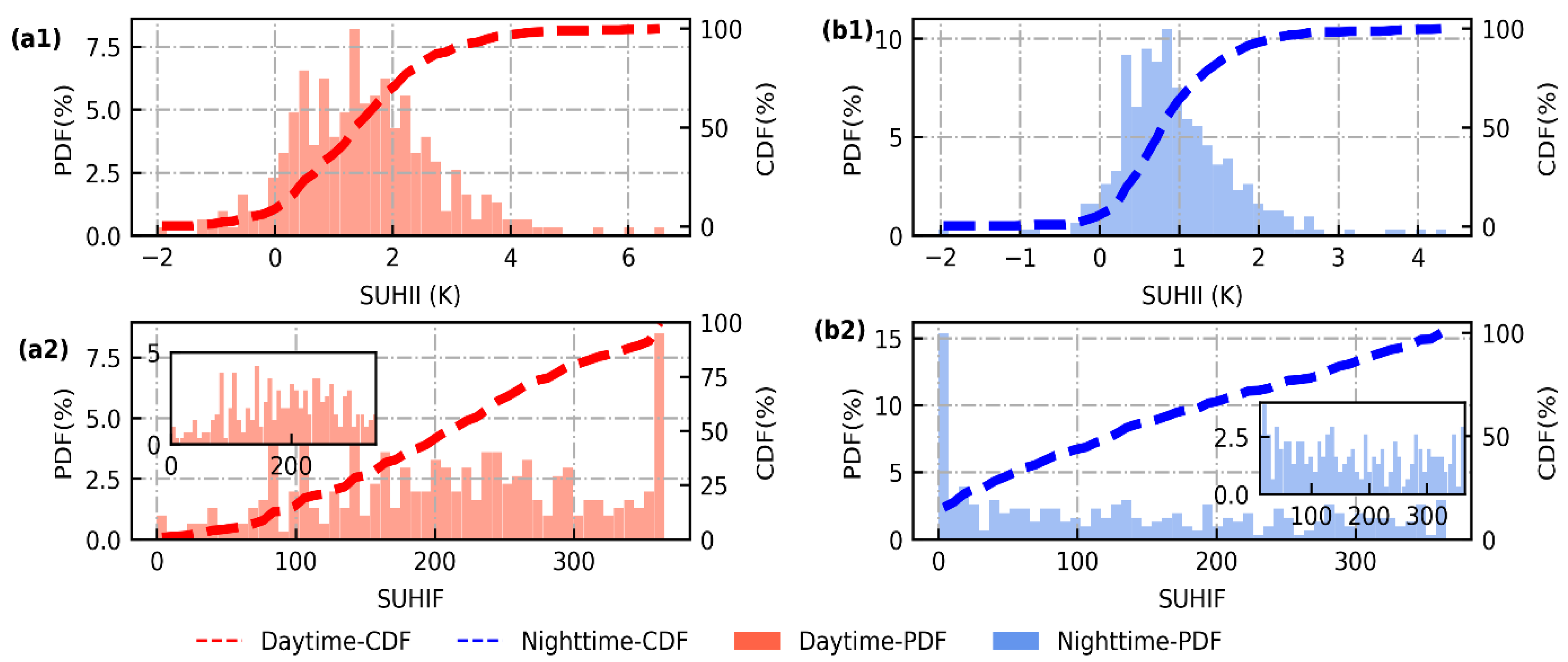
To compare temporal patterns between SUHII and SUHIF, annual and seasonal variations were conducted. Figure 5 shows the Probability Distribution Function (PDF) and Cumulative Distribution Function (CDF) of SUHII and SUHIF across the selected cities. Daytime SUHII is primarily found between 0 and 4 K with an average of 1.53 K. As Zhou et al. [5] reported that UHI largely challenged the ecological environment and human health in China, we found that more than 66.87% of Chinese cities suffer from SUHII over 1 K. Nighttime SUHII, mainly varying from 0 to 2 K with an average of 0.95 K, is less evident than the daytime one. This diurnal contrast was also reported in some previous large-scale studies [6,8,9]. This contrast is possibly attributed to more driving factors for daytime SUHI than for the nighttime one [8]. Additionally, rather than an approximate Gaussian distribution of SUHII, the CDF and PDF of SUHIF indicate different patterns. There is an aggregation in the highest value range (from 354 to 365) accounting for 8.50% of daytime SUHIF. Conversely, nighttime SUHIF shows an aggregation within the lowest value range, accounting for 15.41%. The annual average of SUHIF is 210.88 and 145.27 at day and night respectively, indicating a strong diurnal contrast. Greater SUHIF is found at day than at night. To explore more detail about SUHIF across China, the extremum is excluded from zooming graphs. PDF of SUHIF in the zooming graphs is found to have an approximately homogeneous distribution, which further illustrates the difference from SUHII.
Figure 6 shows the seasonal variations of SHUII and SUHIF on the basis of both seasonal average and value distribution, to provide more information and details. At daytime, SUHII indicates evident seasonal variations. Over four seasons, SUHII over 1 K accounts for 63.93%, 92.78%, 58.36%, and 25.90%, respectively. The strongest season of SUHII is found in summer, with an average of 3.01 K, while the weakest one is found in winter with 0.39 K. Summer daytime is also widely reported to be the strongest season of SUHII in a large number of related studies [5], which is possibly attributed to a strong and negative correlation between ΔEVI and SUHII in the summer [34]. Nevertheless, less evident seasonal variations are observed from nighttime SUHII. Summer, with an average of 1.05 K, is found to be the strongest season, while winter with 0.83 K is found to be the weakest one. This seasonal contrast is also found in some SUHII studies at a global scale [6,8]. Additionally, daytime SUHIF indicates significant seasonal variations, also referred to as being strongest in summer and weakest in winter. SUHIF over 80 days in a season (about 90 days) accounts for about 70.16% of the selected cities in summer, while a SUHIF less than 20 accounts for 60.32% in winter. For both daytime SUHII and SUHIF, the extremums are found in summer and winter, while transition seasons (spring and autumn) are found to have similar variations to each other. Tan et al. [54] reported that daytime SUHI in summer was responsible for the exacerbation of heat waves and was closely associated with heat-related mortality. Thus, the summer SUHI at day, with a strong intensity (3.01 K) and high frequency (80), should be further explored in terms of driving factors and mitigation measurements. At night, a similar average of SUHIF during four seasons (36, 37, 38 and 31) indicates less evident seasonal variations.
4.3. Pattern Classification Based on SUHII and SUHIF
After comparing their spatial and temporal variations between SUHII and SUHIF across 305 Chinese cities, further exploration was conducted to determine their relationship and to conduct a pattern classification (Figure 7). Scatter plots based on SUHII and SUHIF show that there is no city with a high intensity and a low frequency of UHI (vice versa). Despite different value distributions based on their PDF, SUHII and SUHIF of the same city are observed to have a relative consistency, especially at night. Accordingly, a city with high SUHI intensity possibly accompanies high frequency. This closer correlation at night results from the less significant variations of nighttime SUHI. In spite of the consistency between SUHII and SUHIF, it is noted that they provide two different aspects of information from quantity and time. Furthermore, the K-means clustering was employed in the attempts of SUHI pattern classification based on these two important features. This pattern classification allows easy characterization and further exploration to determine whether driving factors vary among these patterns. Three categories, namely the low, medium, and high patterns, are not only proven by the gap statistics as a rational number of classification, but are also meaningful to related researchers and decision-makers. The amount of the selected cities in these three classes is 89, 123, and 93 at day, and 124, 94, and 87 at night. To further explore the discrepancy of these patterns, grouped statistics were conducted. At day, the average of SUHII among these three classes is 0.18 K, 1.49 K, and 2.89 K, and that of SUHIF is 94.06, 210.62, and 323.01. At night, SUHII of three patterns is 0.35 K, 0.93 K, and 1.82 K, and SUHIF is 28.84, 154.31, and 301.46. Cities labelled into the high pattern, of which intensity and frequency are found to be much higher than the average of them all, should attract more attention in both research and practice.
Figure 8 shows the spatial distribution of these SUHI patterns in three aspects, namely the overall, latitudinal, and climate zone-based variations. On the whole, cities labelled as the high pattern at daytime are densely located in the south of China, while those of the low one are primarily located in the northern regions. At night, cities of the high pattern are distributed in the north, while the low ones are mainly in the southern regions. Although a distribution of the two extreme patterns differ to each other, cities of the medium pattern are scattered across China at both day and night. Only 86 cities are found to have consistency patterns during the whole day, and most of the cities accounting for about 71% are found to have a pattern transformation from day to night. This significant diurnal contrast can be possibly attributed to different driving mechanisms of UHI at day and night, which has been widely reported in previous studies [6,17,33,35]. Furthermore, latitudinal variations of patterns show that cities of the low pattern are mainly located in the 35–50° N zone at day, while those of the high ones are densely distributed from 25° to 35°. Apart from scatter distribution, cities of the medium pattern are further observed to have an aggregation of around 35° N based on the quantitative analysis of their latitudinal variations. At night, these three patterns are densely distributed in 45° N, 35° N, and 35° N, respectively. Moreover, almost all of cities grouped into the daytime high pattern are aggregated in the SM climate, according to the climate zone-based variations. Therefore, the climate characteristics of SM are closely associated with high intensity and frequency of SUHI. This close relation between SM and the high pattern of SUHI is possibly due to daytime SUHI being reported to be stronger in humid-hot regions than in cold-drier ones [6,7,10]. Conversely, there is no complete aggregation of any patterns in one climate zone at night.
4.4. Factor Analysis of SUHII and SUHIF
To compare the controls between SUHII and SUHIF, and to further explore pattern effects on controls, the factor analysis was conducted based on SUHII (Figure 9), SUHIF (Figure 10) and pattern classifications (Figure 11), respectively.
Figure 9 shows the correlation between SUHII and potential factors in terms of a daily scale. As great challenges on the reconstruction of daily seamless LST, few factor analyses are conducted on a daily scale. Thanks to the publication of daily all-weather LSTs, this paper can provide insights into daily-scale analysis of their relationship. At day, ΔEVI is found to have a significant correlation with daily SUHII. To make the EVI difference between urban and rural clear, ΔEVI is taken as its absolute value. Accordingly, a positive correlation in this paper is consistent with a negative one in previous studies [8,9]. Vegetation has been widely recognized to have an important cooling factor [6,8,34,54,55], owing to its evapotranspiration. Despite its significance on almost every day of the year (342 days), their correlation coefficients indicate a fluctuation with higher relations in the two transition seasons. This annual fluctuation of the effects from ΔEVI is also found in the studies of driving factors across highly populated cities across eastern China, as proposed by Zhou et al. [9] Temperature and total precipitation are taken as indicators for background climates across the selected cities, which have been reported as important controls for UHI [33,36]. A closer correlation between TP and daytime SUHII throughout the year compared to that in previous studies possibly results from all-weather rather than clear-sky LST employed in this paper. At night, populations in the selected cities indicates the continuous effects on SUHII. Chakraborty and Lee [8] reported that heat storage and anthropogenic heat emission (AHE) were closely related to nighttime UHI. A close association between population and AHE [56] explains the impacts from population on nighttime SUHII. Besides, an evident diurnal contrast from factor correlation is consistent with previous studies of UHI controls [6,9,51].
Figure 10 shows the correlation between SUHIF and potential factors at annual and seasonal scales. At daytime, ΔEVI and TP are found to be significantly correlated to SUHIF, in particular in spring and autumn. Since ΔEVI is an associated indicator for energy transfer between urban and rural environments, it influences not only SUHII, but also its frequency. SUHIF is found to be closely correlated to precipitation at an annual scale. In previous studies, the temporal aggregation of clear-sky data was biased sampling with an ignorance of weather conditions. Here, SUHIF, on the basis of all-weather rather than clear-sky LST, makes it possible to analyze the relationship between it and precipitation. Manoli et al. [36] reported that precipitation influences the UHI based on changes in evapotranspiration and convection efficiency. This close relationship suggests that precipitation makes a strong contribution not only to the magnitude, but also to the frequency. There are two reasons why the effects from ΔEVI and precipitation are more significant in the transition seasons than in summer and winter. First, saturation of daytime SUHIF at summer across most of the selected cities results in a weaker correlation with continuous variables like ΔEVI and precipitation. In winter, a dense aggregation of around zero also influences the factor analysis. Secondly, there are other potential factors that contribute to variations in SUHIF. At night, the relationships between SUHIF and these factors is observed to have less seasonal variations than daytime ones. This is possibly as a result of the non-significant seasonal variations of SUHIF at nighttime. Population is related to daytime SUHIF throughout the year, whereas NTL is correlated to the nighttime one.
After exploring controls for SUHII and SUHIF respectively, comparisons on factor analysis were conducted on the basis of pattern classification at annual and seasonal scales (Figure 11). Two objectives are a comparisons on the controls of SUHII and SUHIF, exploration on temporal variations and pattern variations of factor analysis. At daytime, ΔEVI and TP indicate a significant correlation to both intensity and frequency at an annual scale, while population is found to be presumably irrelevant to their variations. ΔEVI and TP are widely reported as important factors for explaining spatial and temporal variations of SUHI [6,9,36]. In spite of the significant correlation at the annual scale, their impacts are observed to have variations between SUHII and SUHIF among different patterns. On an annual scale, ΔEVI indicates a closer relationship to SUHII, while temperature and precipitation indicate a closer relationship to SUHIF. The frequency is estimated on the basis of daily all-weather LST, which receives considerable impacts from weather conditions. In the cities classified into the high pattern, vegetation is found to be an important factor for daytime SUHII, whereas a much lesser correlation is found in the low and medium patterns. At night, the weak explanation of the selected factors suggest the necessity of a further exploration into the driving factors for nighttime SUHII and SUHIF. Additionally, the factor analysis shows evident seasonal variations. At daytime, there are greater impacts from three important factors (ΔEVI, T and TP) on both SUHII and SUHIF in spring and autumn, rather than during the extreme seasons. In particular, the cities labelled as the high patterns in summer, possibly coupled with heat waves to pose great threats on residential health [57], needs a more comprehensive factor analysis for further mitigations.
5. Conclusions
Great efforts have been devoted to the study of spatiotemporal variations and driving mechanisms of SUHI from the local to the global scale, due to its close association with environmental issues and human health. However, studies on SUHIF are largely challenged by a great number of missing LSTs on a daily scale. There are three issues concerning SUHIF which remain largely unknown, namely its spatiotemporal variations, pattern classifications, and driving factors. Additionally, it is unclear whether SUHII and SUHIF are consistent or different to each other in terms of their variations and controls. Thanks to the release of daily all-weather LSTs across China, this paper is allowed to conduct comparisons between SUHII and SUHIF, to conduct a pattern classification and to further explore their controls.
There are four major findings, which are summarized as follows. First, SUHIF indicates a different north–south contrast between day and night. Cities within the latitude of 20° N to 40° N should be have more attention paid to them, since they are found to have a strong intensity and a high frequency during the day. Despite the overall consistency of spatial distribution, discrepancy between SUHII and SUHIF is observed from the climate zone-based variations, especially at night. Second, SUHIF shows a significant diurnal and seasonal contrast. The difference in SUHIF between day and night is 65.61, while for SUHII it is 0.58 K. Summer daytime is found to have the highest intensity and frequency. Third, the selected 305 Chinese cities are grouped into three patterns based on K-means clustering. After comparative analysis, SUHIF is possibly consistent with SUHII in the same city. Despite the generally similar spatiotemporal patterns between SUHII and SUHIF, they provide quantitative and temporal characteristics, respectively. Fourth, impacts from driving factors on SUHII and SUHIF are found to have significant variations among different times and patterns. Daytime SUHIF is found to be closely associated with precipitation in spring and autumn.
In summer, strong urban heat island and heat waves are reported as great contributors for high heat-related mortality. Therefore, cities classified into the high pattern with both strong intensity and high frequency during summer should be taken as a research emphasis in future exploration, to propose targeting mitigation measurements.
Author Contributions
Conceptualization, K.L. and Y.C.; Methodology, K.L.; Formal Analysis, K.L.; Investigation, K.L.; Data K.L. and S.G.; Writing—Original Draft Preparation, K.L.; Writing—Review and Editing, K.L.; Visualization, K.L.; Supervision, Y.C.; Project Administration, Y.C.; Funding Acquisition, Y.C. All authors have read and agreed to the published version of the manuscript.
Funding
This work was supported by Beijing Natural Science Foundation (8192025), National Key R&D Program of China (2017YFC1502406), Projects of Beijing Advanced Innovation Center for Future Urban Design, Beijing University of Civil Engineering and Architecture (UDC2019031321), and in part by the Beijing Laboratory of Water Resources Security and Beijing Key Laboratory of Environmental Remote Sensing and Digital Cities.
Data Availability Statement
Not applicable.
Acknowledgments
The authors would like to thank Center for Geodata and Analysis, Faculty of Geographical Science, and Beijing Normal University for the high-performance computing support.
Conflicts of Interest
The authors declare that they have no known competing financial interests or personal relationships that could have appeared to influence the work reported in this paper.
References
- United Nations Population Division. The World’s Cities in 2018 Data Booklet; United Nations Population Division: New York, NY, USA, 2018. [Google Scholar]
- Grimm, N.B.; Faeth, S.H.; Golubiewski, N.E.; Redman, C.L.; Wu, J.; Bai, X.; Briggs, J.M. Global Change and the Ecology of Cities. Science 2008, 319, 756–760. [Google Scholar] [CrossRef] [Green Version]
- Li, Y.; Schubert, S.; Kropp, J.P.; Rybski, D. On the influence of density and morphology on the Urban Heat Island intensity. Nat. Commun. 2020, 11, 2647. [Google Scholar] [CrossRef]
- Oke, T.R. The urban energy balance. Prog. Phys. Geogr. Earth Environ. 1988, 12, 471–508. [Google Scholar] [CrossRef]
- Zhou, D.; Xiao, J.; Bonafoni, S.; Berger, C.; Deilami, K.; Zhou, Y.; Frolking, S.; Yao, R.; Qiao, Z.; Sobrino, J.A. Satellite Remote Sensing of Surface Urban Heat Islands: Progress, Challenges, and Perspectives. Remote Sens. 2018, 11, 48. [Google Scholar] [CrossRef] [Green Version]
- Peng, S.; Piao, S.; Ciais, P.; Friedlingstein, P.; Ottle, C.; Bréon, F.-M.; Nan, H.; Zhou, L.; Myneni, R. Surface Urban Heat Island Across 419 Global Big Cities. Environ. Sci. Technol. 2011, 46, 696–703. [Google Scholar] [CrossRef] [PubMed]
- Imhoff, M.L.; Zhang, P.; Wolfe, R.; Bounoua, L. Remote sensing of the urban heat island effect across biomes in the continental USA. Remote Sens. Environ. 2010, 114, 504–513. [Google Scholar] [CrossRef] [Green Version]
- Chakraborty, T.; Lee, X. A simplified urban-extent algorithm to characterize surface urban heat islands on a global scale and examine vegetation control on their spatiotemporal variability. Int. J. Appl. Earth Obs. Geoinf. 2019, 74, 269–280. [Google Scholar] [CrossRef]
- Zhou, D.; Bonafoni, S.; Zhang, L.; Wang, R. Remote sensing of the urban heat island effect in a highly populated urban agglomeration area in East China. Sci. Total Environ. 2018, 628–629, 415–429. [Google Scholar] [CrossRef] [PubMed]
- Peng, J.; Ma, J.; Liu, Q.; Liu, Y.; Hu, Y.; Li, Y.; Yue, Y. Spatial-temporal change of land surface temperature across 285 cities in China: An urban-rural contrast perspective. Sci. Total Environ. 2018, 635, 487–497. [Google Scholar] [CrossRef]
- Yang, Q.; Huang, X.; Tang, Q. The footprint of urban heat island effect in 302 Chinese cities: Temporal trends and associated factors. Sci. Total Environ. 2019, 655, 652–662. [Google Scholar] [CrossRef]
- Santamouris, M. Analyzing the heat island magnitude and characteristics in one hundred Asian and Australian cities and regions. Sci. Total Environ. 2015, 512–513, 582–598. [Google Scholar] [CrossRef]
- Zhou, D.; Zhang, L.; Hao, L.; Sun, G.; Liu, Y.; Zhu, C. Spatiotemporal trends of urban heat island effect along the urban development intensity gradient in China. Sci. Total Environ. 2016, 544, 617–626. [Google Scholar] [CrossRef]
- Azevedo, J.A.; Chapman, L.; Muller, C.L. Quantifying the Daytime and Night-Time Urban Heat Island in Birmingham, UK: A Comparison of Satellite Derived Land Surface Temperature and High Resolution Air Temperature Observations. Remote Sens. 2016, 8, 153. [Google Scholar] [CrossRef] [Green Version]
- Fabrizi, R.; Bonafoni, S.; Biondi, R. Satellite and Ground-Based Sensors for the Urban Heat Island Analysis in the City of Rome. Remote Sens. 2010, 2, 1400–1415. [Google Scholar] [CrossRef] [Green Version]
- Huang, W.; Li, J.; Guo, Q.; Mansaray, L.R.; Li, X.; Huang, J. A Satellite-Derived Climatological Analysis of Urban Heat Island over Shanghai during 2000–2013. Remote Sens. 2017, 9, 641. [Google Scholar] [CrossRef] [Green Version]
- Cao, C.; Lee, X.; Liu, S.; Schultz, N.; Xiao, W.; Zhang, M.; Zhao, L. Urban heat islands in China enhanced by haze pollution. Nat. Commun. 2016, 7, 12509. [Google Scholar] [CrossRef]
- Čeplová, N.; Kalusová, V.; Lososová, Z. Effects of settlement size, urban heat island and habitat type on urban plant biodiversity. Landsc. Urban Plan. 2017, 159, 15–22. [Google Scholar] [CrossRef]
- Santamouris, M. Cooling the cities—A review of reflective and green roof mitigation technologies to fight heat island and improve comfort in urban environments. Sol. Energy 2014, 103, 682–703. [Google Scholar] [CrossRef]
- Li, X.; Zhou, Y.; Yu, S.; Jia, G.; Li, H.; Li, W. Urban heat island impacts on building energy consumption: A review of approaches and findings. Energy 2019, 174, 407–419. [Google Scholar] [CrossRef]
- Wong, K.; Paddon, A.; Jimenez, A. Review of World Urban Heat Islands: Many Linked to Increased Mortality. J. Energy Resour. Technol. 2013, 135, 022101. [Google Scholar] [CrossRef]
- Van Hove, L.; Jacobs, C.; Heusinkveld, B.; Elbers, J.; van Driel, B.; Holtslag, B. Temporal and spatial variability of urban heat island and thermal comfort within the Rotterdam agglomeration. Build. Environ. 2015, 83, 91–103. [Google Scholar] [CrossRef] [Green Version]
- Dong, J.; Peng, J.; He, X.; Corcoran, J.; Qiu, S.; Wang, X. Heatwave-induced human health risk assessment in megacities based on heat stress-social vulnerabil-ity-human exposure framework. Landsc. Urban Plan. 2020, 203, 103907. [Google Scholar] [CrossRef]
- Oke, T.R. The energetic basis of the urban heat island. Q. J. R. Meteorol. Soc. 1982, 108, 1–24. [Google Scholar] [CrossRef]
- Voogt, J.A.; Oke, T.R. Thermal remote sensing of urban climates. Remote Sens. Environ. 2003, 86, 370–384. [Google Scholar] [CrossRef]
- Li, X.; Zhou, X.; Asrar, G.R.; Imhoff, M.; Li, X. The surface urban heat island response to urban expansion: A panel analysis for the conterminous United States. Sci. Total Environ. 2017, 605–606, 426–435. [Google Scholar] [CrossRef] [PubMed]
- Rao, P.K. Remote sensing of urban “heat islands” from an environmental satellite. B. Am. Meteorol. Soc. 1972, 53, 647–648. [Google Scholar]
- Streutker, D. Satellite-measured growth of the urban heat island of Houston, Texas. Remote Sens. Environ. 2003, 85, 282–289. [Google Scholar] [CrossRef]
- Weng, Q.; Lu, D.; Schubring, J. Estimation of land surface temperature–vegetation abundance relationship for urban heat island studies. Remote Sens. Environ. 2004, 89, 467–483. [Google Scholar] [CrossRef]
- Weng, Q. Thermal infrared remote sensing for urban climate and environmental studies: Methods, applications, and trends. ISPRS J. Photogramm. Remote Sens. 2009, 64, 335–344. [Google Scholar] [CrossRef]
- Schwarz, N.; Lautenbach, S.; Seppelt, R. Exploring indicators for quantifying surface urban heat islands of European cities with MODIS land surface temperatures. Remote Sens. Environ. 2011, 115, 3175–3186. [Google Scholar] [CrossRef]
- Quan, J.; Chen, Y.; Zhan, W.; Wang, J.; Voogt, J.; Wang, M. Multi-temporal trajectory of the urban heat island centroid in Beijing, China based on a Gaussian volume model. Remote Sens. Environ. 2014, 149, 33–46. [Google Scholar] [CrossRef]
- Zhao, L.; Lee, X.; Smith, R.B.; Oleson, K. Strong contributions of local background climate to urban heat islands. Nat. Cell Biol. 2014, 511, 216–219. [Google Scholar] [CrossRef]
- Zhou, D.; Zhao, S.; Liu, S.; Zhang, L.; Zhu, C. Surface urban heat island in China’s 32 major cities: Spatial patterns and drivers. Remote Sens. Environ. 2014, 152, 51–61. [Google Scholar] [CrossRef]
- Lai, J.; Zhan, W.; Huang, F.; Voogt, J.; Bechtel, B.; Allen, M.; Peng, S.; Hong, F.; Liu, Y.; Du, P. Identification of typical diurnal patterns for clear-sky climatology of surface urban heat islands. Remote Sens. Environ. 2018, 217, 203–220. [Google Scholar] [CrossRef]
- Manoli, G.; Fatichi, S.; Schläpfer, M.; Yu, K.; Crowther, T.W.; Meili, N.; Burlando, P.; Katul, G.; Bou-Zeid, E. Magnitude of urban heat islands largely explained by climate and population. Nat. Cell Biol. 2019, 573, 55–60. [Google Scholar] [CrossRef] [PubMed]
- Li, X.; Zhou, Y.; Asrar, G.R.; Zhu, Z. Creating a seamless 1 km resolution daily land surface temperature dataset for urban and surrounding areas in the conterminous United States. Remote Sens. Environ. 2018, 206, 84–97. [Google Scholar] [CrossRef]
- Liu, Z.; Zhan, W.; Lai, J.; Hong, F.; Quan, J.; Bechtel, B.; Huang, F.; Zou, Z. Balancing prediction accuracy and generalization ability: A hybrid framework for modelling the annual dynamics of satellite-derived land surface temperatures. ISPRS J. Photogramm. Remote Sens. 2019, 151, 189–206. [Google Scholar] [CrossRef]
- Zhang, X.; Zhou, J.; Liang, S.; Wang, D. A practical reanalysis data and thermal infrared remote sensing data merging (RTM) method for reconstruction of a 1-km all-weather land surface temperature. Remote Sens. Environ. 2021, 260, 112437. [Google Scholar] [CrossRef]
- Zhang, X.; Zhou, J.; Gottsche, F.-M.; Zhan, W.; Liu, S.; Cao, R. A Method Based on Temporal Component Decomposition for Estimating 1-km All-Weather Land Surface Temperature by Merging Satellite Thermal Infrared and Passive Microwave Observations. IEEE Trans. Geosci. Remote Sens. 2019, 57, 4670–4691. [Google Scholar] [CrossRef]
- Li, K.; Chen, Y.; Xia, H.; Gong, A.; Guo, Z. Adjustment From Temperature Annual Dynamics for Reconstructing Land Surface Temperature Based on Downscaled Microwave Observations. IEEE J. Sel. Top. Appl. Earth Obs. Remote Sens. 2020, 13, 5272–5283. [Google Scholar] [CrossRef]
- Duan, S.-B.; Li, Z.-L.; Leng, P. A framework for the retrieval of all-weather land surface temperature at a high spatial resolution from polar-orbiting thermal infrared and passive microwave data. Remote Sens. Environ. 2017, 195, 107–117. [Google Scholar] [CrossRef]
- Kou, X.; Jiang, L.; Bo, Y.; Yan, S.; Chai, L. Estimation of Land Surface Temperature through Blending MODIS and AMSR-E Data with the Bayesian Maximum Entropy Method. Remote Sens. 2016, 8, 105. [Google Scholar] [CrossRef] [Green Version]
- Sun, L.; Chen, Z.; Gao, F.; Anderson, M.; Song, L.; Wang, L.; Hu, B.; Yang, Y. Reconstructing daily clear-sky land surface temperature for cloudy regions from MODIS data. Comput. Geosci. 2017, 105, 10–20. [Google Scholar] [CrossRef]
- Xia, H.; Chen, Y.; Gong, A.; Li, K.; Liang, L.; Guo, Z. Modeling Daily Temperatures Via a Phenology-Based Annual Temperature Cycle Model. IEEE J. Sel. Top. Appl. Earth Obs. Remote Sens. 2021, 14, 6219–6229. [Google Scholar] [CrossRef]
- Li, K.; Chen, Y.; Wang, M.; Gong, A. Spatial-temporal variations of surface urban heat island intensity induced by different definitions of rural extents in China. Sci. Total Environ. 2019, 669, 229–247. [Google Scholar] [CrossRef]
- Wenbin, T.; Zhou, J.; Zhang, X.; Zhang, X.; Ma, J.; Ding, L. Daily 1-km All-Weather Land Surface Temperature Dataset for the Chinese Landmass and Its Surrounding Areas (TRIMS LST; 2000-2020); National Tibetan Plateau Data Center: Beijing, China, 2021. [Google Scholar]
- Zhou, J.; Zhang, X.; Zhan, W.; Goettsche, F.-M.; Liu, S.; Olesen, F.-S.; Hu, W.; Dai, F. A Thermal Sampling Depth Correction Method for Land Surface Temperature Estimation from Satellite Passive Microwave Observation Over Barren Land. IEEE Trans. Geosci. Remote Sens. 2017, 55, 4743–4756. [Google Scholar] [CrossRef]
- Lai, J.; Zhan, W.; Huang, F.; Quan, J.; Hu, L.; Gao, L.; Ju, W. Does quality control matter? Surface urban heat island intensity variations estimated by satellite-derived land surface temperature products. ISPRS J. Photogramm. Remote Sens. 2018, 139, 212–227. [Google Scholar] [CrossRef]
- Likas, A.; Vlassis, N.; Verbeek, J.J. The global k-means clustering algorithm. Pattern Recognit. 2003, 36, 451–461. [Google Scholar] [CrossRef] [Green Version]
- Li, L.; Zha, Y.; Zhang, J. Spatially non-stationary effect of underlying driving factors on surface urban heat islands in global major cities. Int. J. Appl. Earth Obs. Geoinf. 2020, 90, 102131. [Google Scholar] [CrossRef]
- Deilami, K.; Kamruzzaman, M.; Liu, Y. Urban heat island effect: A systematic review of spatio-temporal factors, data, methods, and mitigation measures. Int. J. Appl. Earth Obs. Geoinf. 2018, 67, 30–42. [Google Scholar] [CrossRef]
- Tan, J.; Zheng, Y.; Tang, X.; Guo, C.; Li, L.; Song, G.; Zhen, X.; Yuan, D.; Kalkstein, A.J.; Li, F.; et al. The urban heat island and its impact on heat waves and human health in Shanghai. Int. J. Biometeorol. 2009, 54, 75–84. [Google Scholar] [CrossRef] [PubMed]
- Clinton, N.; Gong, P. MODIS detected surface urban heat islands and sinks: Global locations and controls. Remote Sens. Environ. 2013, 134, 294–304. [Google Scholar] [CrossRef]
- Zhou, W.; Wang, J.; Cadenasso, M.L. Effects of the spatial configuration of trees on urban heat mitigation: A comparative study. Remote Sens. Environ. 2017, 195, 1–12. [Google Scholar] [CrossRef]
- Flanner, M.G. Integrating anthropogenic heat flux with global climate models. Geophys. Res. Lett. 2009, 36, 36. [Google Scholar] [CrossRef] [Green Version]
- Founda, D.; Santamouris, M. Synergies between Urban Heat Island and Heat Waves in Athens (Greece), during an extremely hot summer (2012). Sci. Rep. 2017, 7, 10973. [Google Scholar] [CrossRef] [Green Version]
Figure 1.
Spatial distribution of the 305 selected cities across China. The background of the map shows Land use and land cover from MODIS MCD12Q1. The bar plot (b) shows the percentage of these cities according to five population classifications.
Figure 1.
Spatial distribution of the 305 selected cities across China. The background of the map shows Land use and land cover from MODIS MCD12Q1. The bar plot (b) shows the percentage of these cities according to five population classifications.

Figure 2.
Flowchart of this study. There are four steps, including SUHII calculation, SUHIF estimation, pattern classification and factor analysis. To make it clear, Tianjin is taken as an example in the flowchart.
Figure 2.
Flowchart of this study. There are four steps, including SUHII calculation, SUHIF estimation, pattern classification and factor analysis. To make it clear, Tianjin is taken as an example in the flowchart.

Figure 3.
Spatial distribution of SUHII and SUHIF at daytime (a) and nighttime (b) in China. The spatial maps in the first row represent SUHII (a1,b1). The second row maps represent SUHIF (a2,b2).
Figure 3.
Spatial distribution of SUHII and SUHIF at daytime (a) and nighttime (b) in China. The spatial maps in the first row represent SUHII (a1,b1). The second row maps represent SUHIF (a2,b2).

Figure 4.
Latitudinal and climate zone-based variations of SUHII and SUHIF at daytime and nighttime. The two maps (a1,b1) show the latitudinal and climatic distributions of the selected cities, respectively. The plots in the first row show latitudinal variations of SUHII (a2,a3) and SUHIF (a4,a5) based on the combination of their average and variance. The violin plots in the second row show climate zone-based variations of SUHII (b2) and SUHIF (b3). The daytime and nighttime patterns are represented based on red and blue colors, respectively.

Figure 5.
Annual variations of SUHII and SUHIF at daytime (a) and nighttime (b). The plots in the first row show the value distribution of annual SUHII (a1,b1), and the second-row plots show that of SUHIF (a2,b2). PDF and CDF are employed to show the value distribution across the selected cities. To clearly show their variations, zoom-in images without the extremum are added for SUHIF.

Figure 6.
Seasonal variations of SUHII and SUHIF at daytime (a) and nighttime (b). The discrete distribution as horizontal bar charts in the first row shows seasonal variations of SUHII (a1,b1) and the second row charts show that of SUHIF (a3,b3). Percentage over 10% is labelled in the graph. The line plots in the first row show the average of SUHII (a2,b2) and plots in the second row show that of SUHIF (a4,b4) among the different seasons.

Figure 7.
Relationship between SUHII and SUHIF at daytime (a) and nighttime (b). The scatter plots show their relationship, with color representation of three categories, namely the low (L), medium (M), and high (H) patterns. To clearly show the characteristics of these three categories, the bar charts show the average of SUHII (a1-R,b1-R) and SUHIF (a1-L,b1-L). The histograms represent the PDF of SUHII (a2,b2) and SUHIF (a3,b3).

Figure 8.
Spatial distribution of the aforementioned three categories at daytime (a) and nighttime (b). The maps show the spatial distribution of three pattern classifications (a1,a2). The line plots show their latitudinal variations (a2,b2). The bar plots show their climate zone-based variations (a3,b3). Different patterns are represented by colors.

Figure 9.
Relationships between SUHII and potential factors at a daily scale. The heat maps represent their correlation at daytime (a1) and nighttime (a2). The bar charts (b) show a diurnal contrast of their relationships in terms of each factor ((b1) for ΔEVI, (b2) for T, (b3) for TP, (b4) for Pop, (b5) for NTL). To make the results clear, the correlation with a p-value less than 0.05 is shown in the bar charts. The fitting lines are employed to clearly show the annual variations in their correlation, where days with p-values less than 0.05 are found to be over 270 during a year.

Figure 10.
Relationship between SUHIF and potential factors in terms of annual and seasonal scales. The heat maps represent their correlation at daytime (a1) and nighttime (a2). The bar charts (b) show a diurnal contrast of their relationship in terms of each factor ((b1) for ΔEVI, (b2) for T, (b3) for TP, (b4) for Pop, (b5) for NTL). To make the results clear, the correlation with p-values less than 0.05 are labeled in the heat maps.

Figure 11.
Comparisons of factor analysis based on SUHII and SUHIF in terms of pattern classifications at daytime (a) and nighttime (b). There are two temporal scales, namely annual and seasonal scales. I is the abbreviation of SUHII and F is the abbreviation of SUHIF. To make the results clear, the correlations with p-value less than 0.05 are labeled in the heat maps.

Publisher’s Note: MDPI stays neutral with regard to jurisdictional claims in published maps and institutional affiliations. |
© 2021 by the authors. Licensee MDPI, Basel, Switzerland. This article is an open access article distributed under the terms and conditions of the Creative Commons Attribution (CC BY) license (https://creativecommons.org/licenses/by/4.0/).
Share and Cite
MDPI and ACS Style
Li, K.; Chen, Y.; Gao, S. Comparative Analysis of Variations and Patterns between Surface Urban Heat Island Intensity and Frequency across 305 Chinese Cities. Remote Sens. 2021, 13, 3505. https://doi.org/10.3390/rs13173505
AMA Style
Li K, Chen Y, Gao S. Comparative Analysis of Variations and Patterns between Surface Urban Heat Island Intensity and Frequency across 305 Chinese Cities. Remote Sensing. 2021; 13(17):3505. https://doi.org/10.3390/rs13173505
Chicago/Turabian StyleLi, Kangning, Yunhao Chen, and Shengjun Gao. 2021. "Comparative Analysis of Variations and Patterns between Surface Urban Heat Island Intensity and Frequency across 305 Chinese Cities" Remote Sensing 13, no. 17: 3505. https://doi.org/10.3390/rs13173505
Note that from the first issue of 2016, this journal uses article numbers instead of page numbers. See further details here.