
Satellite Retrieval of Microwave Land Surface Emissivity under Clear and Cloudy Skies in China Using Observations from AMSR-E and MODIS

 , ,
, ,  , , and
Abstract
:
1. Introduction
2. Datasets
2.1. Input Data
2.2. Validation Data
2.3. Ancillary Data
3. Methods of MLSE Retrieval
3.1. Radiative Transfer Model
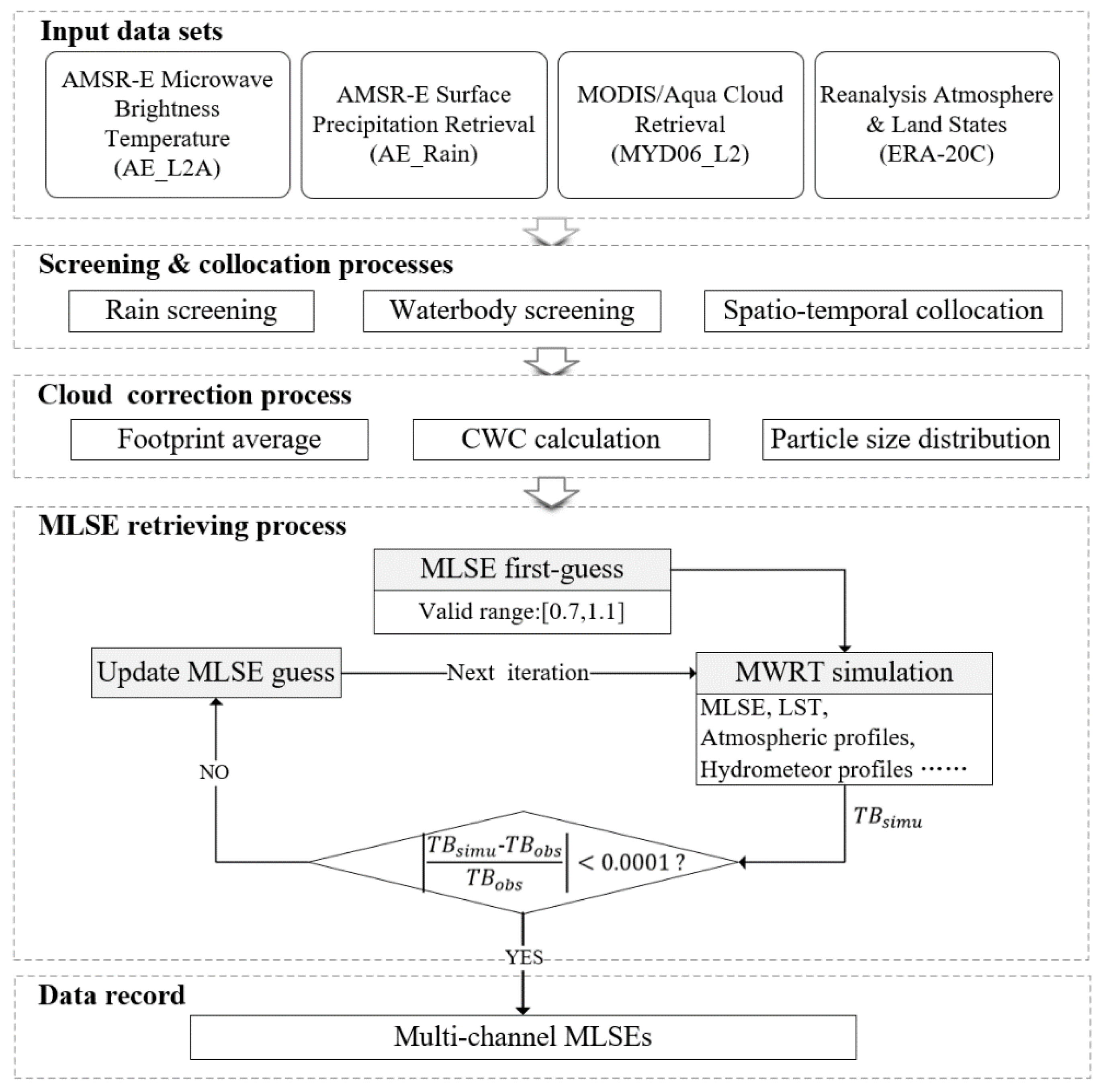
3.2. Descriptions of Retrieval Algorithm of MLSE
3.3. Validations of Inputs
3.4. Sensitivity Tests
4. Results
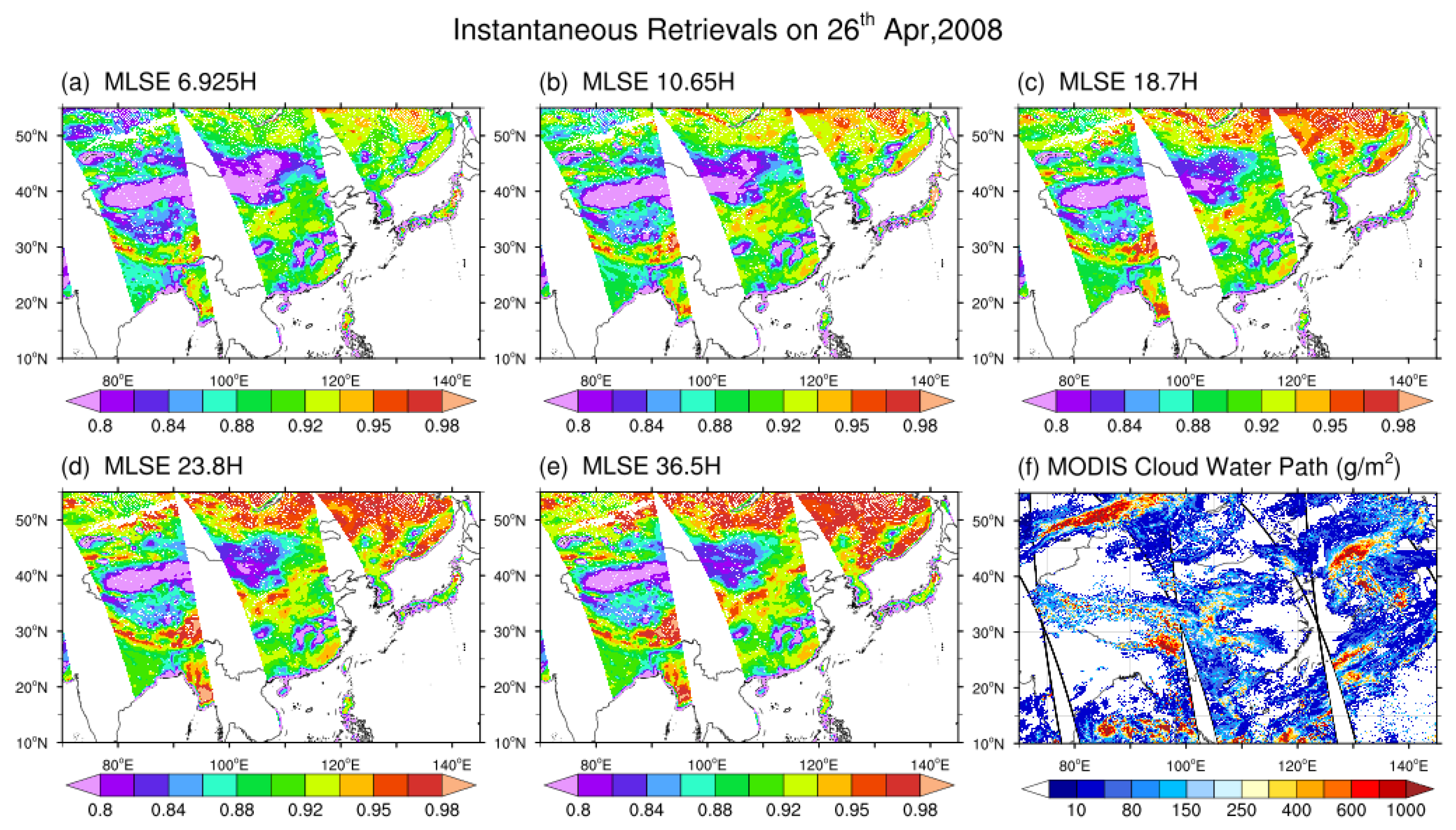
4.1. Retrieval of Instantaneous MLSE
4.2. Spatial Distribution of MLSE
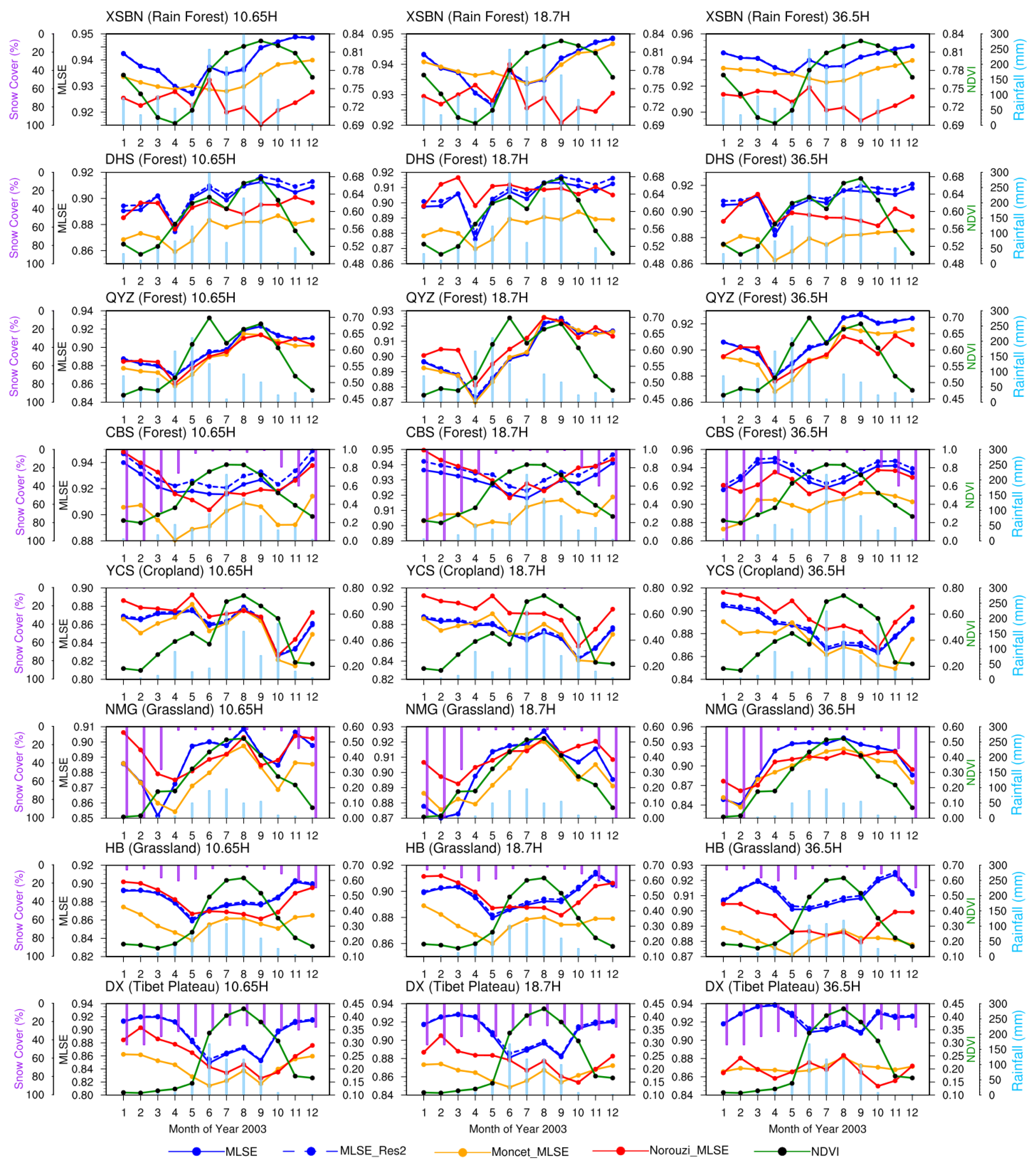
4.3. Seasonal Variation and Potential Controlling Factors of MLSE
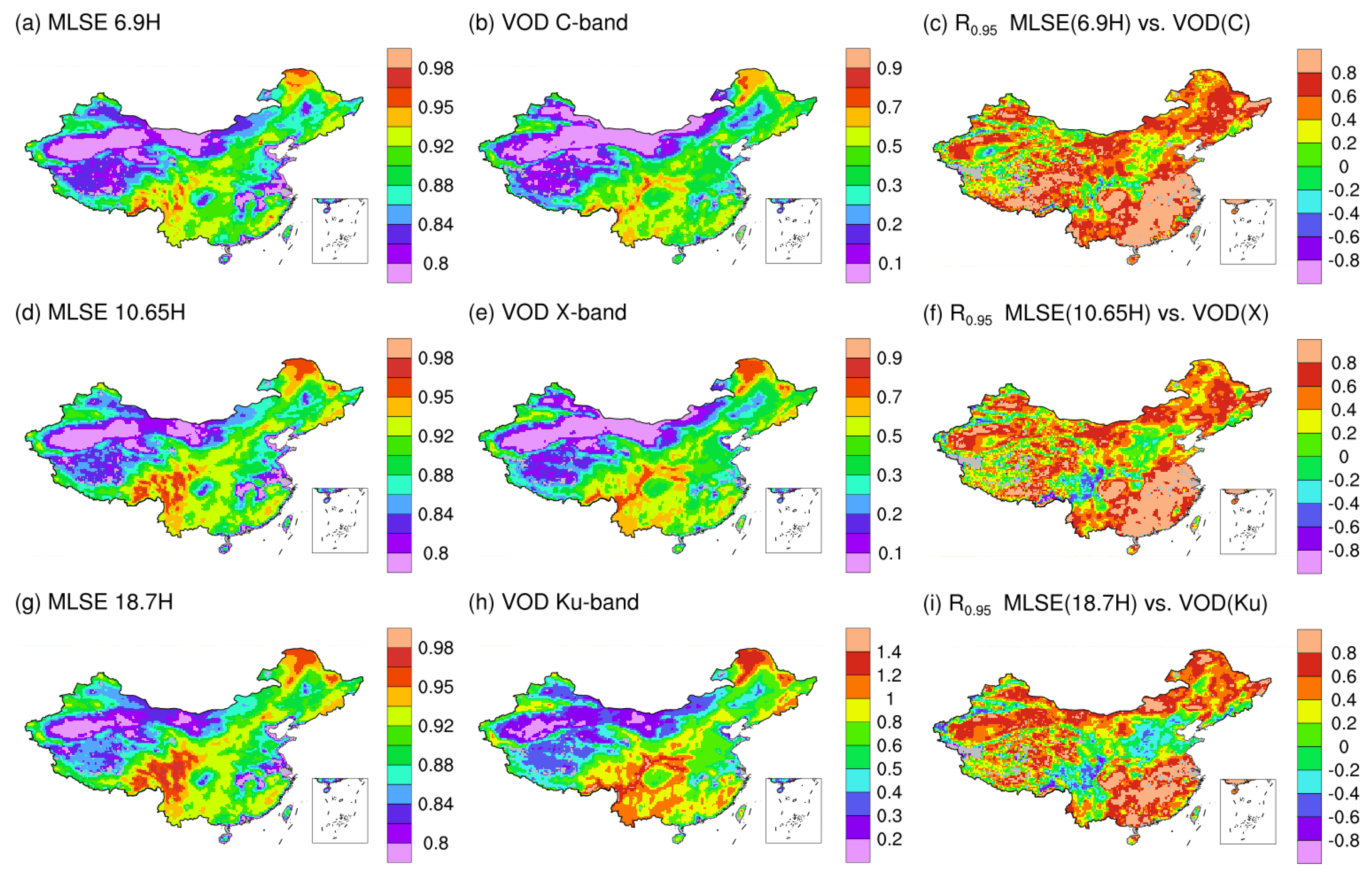
4.4. Comparison with Microwave Vegetation Optical Depth (VOD)
5. Discussion
5.1. Comparing with Similar Works in the Literature
5.2. Error Sources
5.3. Potential Applications
6. Summary and Conclusions
Supplementary Materials
Author Contributions
Funding
Data Availability Statement
Acknowledgments
Conflicts of Interest
References
- Weng, F.; Yan, B.; Grody, N.C. A microwave land emissivity model. J. Geophys. Res. Space Phys. 2001, 106, 20115–20123. [Google Scholar] [CrossRef]
- Njoku, E.; Jackson, T.; Lakshmi, V.; Chan, T.; Nghiem, S. Soil moisture retrieval from AMSR-E. IEEE Trans. Geosci. Remote Sens. 2003, 41, 215–229. [Google Scholar] [CrossRef]
- Jones, L.A.; Kimball, J.S.; McDonald, K.C.; Chan, S.T.K.; Njoku, E.G.; Oechel, W. Satellite Microwave Remote Sensing of Boreal and Arctic Soil Temperatures From AMSR-E. IEEE Trans. Geosci. Remote Sens. 2007, 45, 2004–2018. [Google Scholar] [CrossRef]
- Min, Q.; Lin, B.; Li, R. Remote Sensing Vegetation Hydrological States Using Passive Microwave Measurements. IEEE J. Sel. Top. Appl. Earth Obs. Remote Sens. 2010, 3, 124–131. [Google Scholar] [CrossRef]
- Ulaby, F.T.; Moore, R.K.; Fung, A.K. Microwave Remote Sensing Active and Passive-Volume III: From Theory to Applications; Artech House: Norwood, MA, USA, 1986. [Google Scholar]
- Moncet, J.-L.; Liang, P.; Galantowicz, J.F.; Lipton, A.E.; Uymin, G.; Prigent, C.; Grassotti, C. Land surface microwave emissivities derived from AMSR-E and MODIS measurements with advanced quality control. J. Geophys. Res. Space Phys. 2011, 116, D16104. [Google Scholar] [CrossRef]
- Baordo, F.; Geer, A.J. Assimilation of SSMIS humidity-sounding channels in all-sky conditions over land using a dynamic emissivity retrieval. Q. J. R. Meteorol. Soc. 2016, 142, 2854–2866. [Google Scholar] [CrossRef]
- Ferraro, R.; Peters-Lidard, C.; Hernandez, C.; Turk, F.J.; Aires, F.; Prigent, C.; Lin, X.; Boukabara, S.A.; Furuzawa, F.A.; Gopalan, K.; et al. An Evaluation of Microwave Land Surface Emissivities Over the Continental United States to Benefit GPM-Era Precipitation Algorithms. IEEE Trans. Geosci. Remote Sens. 2012, 51, 378–398. [Google Scholar] [CrossRef]
- Harrison, K.W.; Tian, Y.; Peters-Lidard, C.; Ringerud, S.; Kumar, S. Calibration to Improve Forward Model Simulation of Microwave Emissivity at GPM Frequencies Over the U.S. Southern Great Plains. IEEE Trans. Geosci. Remote Sens. 2016, 54, 1103–1117. [Google Scholar] [CrossRef] [Green Version]
- Turk, F.J.; Ringerud, S.E.; You, Y.; Camplani, A.; Casella, D.; Panegrossi, G.; Sanò, P.; Ebtehaj, A.; Guilloteau, C.; Utsumi, N.; et al. Adapting Passive Microwave-Based Precipitation Algorithms to Variable Microwave Land Surface Emissivity to Improve Precipitation Estimation from the GPM Constellation. J. Hydrometeorol. 2021, 22, 1755–1781. [Google Scholar] [CrossRef]
- Min, Q.; Lin, B. Determination of spring onset and growing season leaf development using satellite measurements. Remote Sens. Environ. 2006, 104, 96–102. [Google Scholar] [CrossRef]
- Min, Q.; Lin, B. Remote sensing of evapotranspiration and carbon uptake at Harvard Forest. Remote Sens. Environ. 2006, 100, 379–387. [Google Scholar] [CrossRef] [Green Version]
- Owe, M.; De Jeu, R.; Holmes, T. Multisensor historical climatology of satellite-derived global land surface moisture. J. Geophys. Res. Space Phys. 2008, 113, F01002. [Google Scholar] [CrossRef]
- Wigneron, J.-P.; Jackson, T.; O’Neill, P.; De Lannoy, G.; de Rosnay, P.; Walker, J.; Ferrazzoli, P.; Mironov, V.; Bircher, S.; Grant, J.; et al. Modelling the passive microwave signature from land surfaces: A review of recent results and application to the L-band SMOS & SMAP soil moisture retrieval algorithms. Remote Sens. Environ. 2017, 192, 238–262. [Google Scholar] [CrossRef]
- Wang, Y.; Li, R.; Min, Q.; Fu, Y.; Wang, Y.; Zhong, L.; Fu, Y. A three-source satellite algorithm for retrieving all-sky evapotranspiration rate using combined optical and microwave vegetation index at twenty AsiaFlux sites. Remote Sens. Environ. 2019, 235, 111463. [Google Scholar] [CrossRef]
- Wang, Y.; Li, R.; Min, Q.; Zhang, L.; Yu, G.; Bergeron, Y. Estimation of Vegetation Latent Heat Flux over Three Forest Sites in ChinaFLUX using Satellite Microwave Vegetation Water Content Index. Remote Sens. 2019, 11, 1359. [Google Scholar] [CrossRef] [Green Version]
- Zhang, Y.; Li, R.; Min, Q.; Bo, H.; Fu, Y.; Wang, Y.; Gao, Z. The Controlling Factors of Atmospheric Formaldehyde (HCHO) in Amazon as Seen from Satellite. Earth Space Sci. 2019, 6, 959–971. [Google Scholar] [CrossRef] [Green Version]
- Forkel, M.; Dorigo, W.; Lasslop, G.; Teubner, I.; Chuvieco, E.; Thonicke, K. A data-driven approach to identify controls on global fire activity from satellite and climate observations (SOFIA V1). Geosci. Model Dev. 2017, 10, 4443–4476. [Google Scholar] [CrossRef] [Green Version]
- Fan, L.; Wigneron, J.-P.; Xiao, Q.; Al-Yaari, A.; Wen, J.; Martin-StPaul, N.; Dupuy, J.-L.; Pimont, F.; Al Bitar, A.; Moran, R.F.; et al. Evaluation of microwave remote sensing for monitoring live fuel moisture content in the Mediterranean region. Remote Sens. Environ. 2018, 205, 210–223. [Google Scholar] [CrossRef]
- Wigneron, J.-P.; Chanzy, A.; Calvet, J.-C.; Bruguier, N. A simple algorithm to retrieve soil moisture and vegetation biomass using passive microwave measurements over crop fields. Remote Sens. Environ. 1995, 51, 331–341. [Google Scholar] [CrossRef]
- Liu, Y.Y.; Van Dijk, A.; De Jeu, R.A.M.; Canadell, J.; McCabe, M.; Evans, J.; Wang, G. Recent reversal in loss of global terrestrial biomass. Nat. Clim. Chang. 2015, 5, 470–474. [Google Scholar] [CrossRef]
- Brandt, M.; Wigneron, J.-P.; Chave, J.; Tagesson, T.; Penuelas, J.; Ciais, P.; Rasmussen, K.; Tian, F.; Mbow, C.; Al-Yaari, A.; et al. Satellite passive microwaves reveal recent climate-induced carbon losses in African drylands. Nat. Ecol. Evol. 2018, 2, 827–835. [Google Scholar] [CrossRef] [PubMed] [Green Version]
- Prigent, C.; Rossow, W.B.; Matthews, E. Microwave land surface emissivities estimated from SSM/I observations. J. Geophys. Res. Space Phys. 1997, 102, 21867–21890. [Google Scholar] [CrossRef]
- Lin, B.; Minnis, P. Temporal Variations of Land Surface Microwave Emissivities over the Atmospheric Radiation Measurement Program Southern Great Plains Site. J. Appl. Meteorol. 2000, 39, 1103–1116. [Google Scholar] [CrossRef]
- Karbou, F.; Prigent, C.; Eymard, L.; Pardo, J.R. Microwave land emissivity calculations using AMSU measurements. IEEE Trans. Geosci. Remote Sens. 2005, 43, 948–959. [Google Scholar] [CrossRef]
- Norouzi, H.; Temimi, M.; Rossow, W.B.; Pearl, C.; Azar, M.; Khanbilvardi, R. The sensitivity of land emissivity estimates from AMSR-E at C and X bands to surface properties. Hydrol. Earth Syst. Sci. 2011, 15, 3577–3589. [Google Scholar] [CrossRef] [Green Version]
- Kalnay, E.; Kanamitsu, M.; Baker, W.E. Global Numerical Weather Prediction at the National Meteorological Center. Bull. Am. Meteorol. Soc. 1990, 71, 1410–1428. [Google Scholar] [CrossRef]
- Rossow, W.B.; Schiffer, R.A. ISCCP Cloud Data Products. Bull. Am. Meteorol. Soc. 1991, 72, 2–20. [Google Scholar] [CrossRef]
- Rossow, W.B.; Schiffer, R.A. Advances in understanding clouds from ISCCP. Bull. Am. Meteorol. Soc. 1999, 80, 2261–2287. [Google Scholar] [CrossRef] [Green Version]
- Aires, F.; Prigent, C.; Rossow, W.B.; Rothstein, M. A new neural network approach including first guess for retrieval of atmospheric water vapor, cloud liquid water path, surface temperature, and emissivities over land from satellite microwave observations. J. Geophys. Res. Space Phys. 2001, 106, 14887–14907. [Google Scholar] [CrossRef]
- Ashcroft, P.; Wentz, F.J. AMSR-E/Aqua L2A Global Swath Spatially-Resampled Brightness Temperatures; Version 3; NASA National Snow and Ice Data Center Distributed Active Archive Center: Boulder, CO, USA, 2013. [CrossRef]
- Ashcroft, P.; Wentz, F.J. Algorithm Theoretical Basis Document (ATBD) AMSR Level 2A Algorithm; Remote Sensing Systems: Santa Rosa, CA, USA, 2000. [Google Scholar]
- Kummerow, C.; Ferraro, R.; Randel, D. AMSR-E/Aqua L2B Global Swath Surface Precipitation GSFC Profiling Algorithm; Version 3; NASA National Snow and Ice Data Center Distributed Active Archive Center: Boulder, CO, USA, 2015. [CrossRef]
- Poli, P.; Hersbach, H.; Dee, D.; Berrisford, P.; Simmons, A.J.; Vitart, F.; Laloyaux, P.; Tan, D.G.H.; Peubey, C.; Thépaut, J.-N.; et al. ERA-20C: An Atmospheric Reanalysis of the Twentieth Century. J. Clim. 2016, 29, 4083–4097. [Google Scholar] [CrossRef]
- Platnick, S.; Ackerman, S.A.; King, M.D.; Meyer, K.; Menzel, W.P.; Holz, R.E.; Baum, B.A.; Yang, P. MODIS Atmosphere L2 Cloud Product (06_L2), NASA MODIS Adaptive Processing System; Goddard Space Flight Center: Greenbelt, MD, USA, 2015. [Google Scholar] [CrossRef]
- Zhang, Q.; Zhao, Y.; Fan, S. Development of hourly precipitation datasets for national meteorological stations in China. Torrential Rain Disasters 2016, 35, 182–186. [Google Scholar]
- Friedl, M.; Sulla-Menashe, D. MCD12C1 MODIS/Terra + Aqua Land Cover Type Yearly L3 Global 0.05Deg CMG V006; NASA EOSDIS Land Processes DAAC: Sioux Falls, SD, USA, 2015.
- Moesinger, L.; Dorigo, W.; de Jeu, R.; van der Schalie, R.; Scanlon, T.; Teubner, I.; Forkel, M. The global long-term microwave Vegetation Optical Depth Climate Archive (VODCA). Earth Syst. Sci. Data 2020, 12, 177–196. [Google Scholar] [CrossRef] [Green Version]
- Didan, K. MYD13C2 MODIS/Aqua Vegetation Indices Monthly L3 Global 0.05Deg CMG V006; NASA EOSDIS Land Processes DAAC: Sioux Falls, SD, USA, 2015. [CrossRef]
- Schneider, U.; Becker, A.; Finger, P.; Meyer-Christoffer, A.; Rudolf, B.; Ziese, M. GPCC Full Data Reanalysis Version 7.0 at 0.5°: Monthly Land-Surface Precipitation from Rain-Gauges built on GTS-based and Historic Data; Global Precipitation Climatology Centre: Offenbach, Germany, 2011. [Google Scholar] [CrossRef]
- Hall, D.K.; Riggs, G.A.; Solomonson, V.; Sips, N.M. MODIS/Aqua Snow Cover Monthly L3 Global 0.05Deg CMG, Version 6; NASA National Snow and Ice Data Center Distributed Active Archive Center: Boulder, CO, USA, 2016. [CrossRef]
- Lin, B.; Wielicki, B.; Minnis, P.; Rossow, W. Estimation of water cloud properties from satellite microwave, infrared and visible measurements in oceanic environments: 1. Microwave brightness temperature simulations. J. Geophys. Res. Space Phys. 1998, 103, 3873–3886. [Google Scholar] [CrossRef]
- Liu, G. A Fast and Accurate Model for Microwave Radiance Calculations. J. Meteorol. Soc. Jpn. 1998, 76, 335–343. [Google Scholar] [CrossRef] [Green Version]
- Liu, G. Approximation of Single Scattering Properties of Ice and Snow Particles for High Microwave Frequencies. J. Atmos. Sci. 2004, 61, 2441–2456. [Google Scholar] [CrossRef]
- Noh, Y.-J.; Liu, G.; Seo, E.-K.; Wang, J.R.; Aonashi, K. Development of a snowfall retrieval algorithm at high microwave frequencies. J. Geophys. Res. Space Phys. 2006, 111, D22216. [Google Scholar] [CrossRef]
- Aonashi, K.; Awaka, J.; Hirose, M.; Kozu, T.; Kubota, T.; Liu, G.; Shige, S.; Kida, S.; Seto, S.; Takahashi, N.; et al. GSMaP Passive Microwave Precipitation Retrieval Algorithm: Algorithm Description and Validation. J. Meteorol. Soc. Jpn. 2009, 87, 119–136. [Google Scholar] [CrossRef] [Green Version]
- Fujii, H.; Koike, T.; Imaoka, K. Improvement of the AMSR-E Algorithm for Soil Moisture Estimation by Introducing a Fractional Vegetation Coverage Dataset Derived from MODIS Data. J. Remote Sens. 2009, 29, 282–292. [Google Scholar] [CrossRef]
- Noh, Y.-J.; Liu, G.; Jones, A.S.; Haar, T.H.V. Toward snowfall retrieval over land by combining satellite and in situ measurements. J. Geophys. Res. Space Phys. 2009, 114, D24205. [Google Scholar] [CrossRef]
- Shige, S.; Yamamoto, T.; Tsukiyama, T.; Kida, S.; Ashiwake, H.; Kubota, T.; Seto, S.; Aonashi, K.; Okamoto, K. The GSMaP Precipitation Retrieval Algorithm for Microwave Sounders—Part I: Over-Ocean Algorithm. IEEE Trans. Geosci. Remote Sens. 2009, 47, 3084–3097. [Google Scholar] [CrossRef]
- Wang, Y.; Fu, Y.; Liu, G.; Liu, Q.; Sun, L. A new water vapor algorithm for TRMM Microwave Imager (TMI) measurements based on a log linear relationship. J. Geophys. Res. Space Phys. 2009, 114, D21304. [Google Scholar] [CrossRef]
- Shige, S.; Kida, S.; Ashiwake, H.; Kubota, T.; Aonashi, K. Improvement of TMI Rain Retrievals in Mountainous Areas. J. Appl. Meteorol. Clim. 2013, 52, 242–254. [Google Scholar] [CrossRef] [Green Version]
- Taniguchi, A.; Shige, S.; Yamamoto, M.; Mega, T.; Kida, S.; Kubota, T.; Kachi, M.; Ushio, T.; Aonashi, K. Improvement of High-Resolution Satellite Rainfall Product for Typhoon Morakot (2009) over Taiwan. J. Hydrometeorol. 2013, 14, 1859–1871. [Google Scholar] [CrossRef] [Green Version]
- Jeoung, H.; Liu, G.; Kim, K.; Lee, G.; Seo, E.-K. Microphysical properties of three types of snow clouds: Implication for satellite snowfall retrievals. Atmospheric Chem. Phys. Discuss. 2020, 20, 14491–14507. [Google Scholar] [CrossRef]
- Kubota, T.; Aonashi, K.; Ushio, T.; Shige, S.; Takayabu, Y.N.; Kachi, M.; Arai, Y.; Tashima, T.; Masaki, T.; Kawamoto, N.; et al. Global Satellite Mapping of Precipitation (GSMaP) Products in the GPM Era. In Satellite Precipitation Measurement; Springer: Richmond, VA, USA, 2020; pp. 355–373. [Google Scholar]
- Ackerman, S.A.; Stephens, G.L. The Absorption of Solar Radiation by Cloud Droplets: An Application of Anomalous Diffraction Theory. J. Atmos. Sci. 1987, 44, 1574–1588. [Google Scholar] [CrossRef] [Green Version]
- Lin, B.; Rossow, W.B. Observations of cloud liquid water path over oceans: Optical and microwave remote sensing methods. J. Geophys. Res. Space Phys. 1994, 99, 20907–20927. [Google Scholar] [CrossRef]
- English, S.J. Airborne radiometric observations of cloud liquid-water emission at 89 and 157 GHz: Application to retrieval of liquid-water path. Q. J. R. Meteorol. Soc. 1995, 121, 1501–1524. [Google Scholar] [CrossRef]
- Zhang, Y.; Rossow, W.B.; Stackhouse, P.W. Comparison of different global information sources used in surface radiative flux calculation: Radiative properties of the near-surface atmosphere. J. Geophys. Res. Space Phys. 2006, 111, D13106. [Google Scholar] [CrossRef]
- Prigent, C.; Aires, F.; Rossow, W.B. Land Surface Microwave Emissivities over the Globe for a Decade. Bull. Am. Meteorol. Soc. 2006, 87, 1573–1584. [Google Scholar] [CrossRef] [Green Version]
- Rosenfeld, S.; Grody, N. Anomalous microwave spectra of snow cover observed from Special Sensor Microwave/Imager measurements. J. Geophys. Res. Space Phys. 2000, 105, 14913–14925. [Google Scholar] [CrossRef]
- Kongoli, C.; Grody, N.C.; Ferraro, R.R. Interpretation of AMSU microwave measurements for the retrievals of snow water equivalent and snow depth. J. Geophys. Res. Space Phys. 2004, 109, D24111. [Google Scholar] [CrossRef]
- Owe, M.; De Jeu, R.; Walker, J. A methodology for surface soil moisture and vegetation optical depth retrieval using the microwave polarization difference index. IEEE Trans. Geosci. Remote Sens. 2001, 39, 1643–1654. [Google Scholar] [CrossRef] [Green Version]
- Holmes, T.R.H.; De Jeu, R.A.M.; Owe, M.; Dolman, A. Land surface temperature from Ka band (37 GHz) passive microwave observations. J. Geophys. Res. Space Phys. 2009, 114, D04113. [Google Scholar] [CrossRef] [Green Version]
- Tian, Y.; Peters-Lidard, C.; Harrison, K.W.; Prigent, C.; Norouzi, H.; Aires, F.; Boukabara, S.A.; Furuzawa, F.A.; Masunaga, H. Quantifying Uncertainties in Land-Surface Microwave Emissivity Retrievals. IEEE Trans. Geosci. Remote Sens. 2013, 52, 829–840. [Google Scholar] [CrossRef]
- Norouzi, H.; Temimi, M.; Prigent, C.; Turk, J.; Khanbilvardi, R.; Tian, Y.; Furuzawa, F.A.; Masunaga, H. Assessment of the consistency among global microwave land surface emissivity products. Atmos. Meas. Tech. 2015, 8, 1197–1205. [Google Scholar] [CrossRef] [Green Version]
- Yang, H.; Weng, F. Error Sources in Remote Sensing of Microwave Land Surface Emissivity. IEEE Trans. Geosci. Remote Sens. 2011, 49, 3437–3442. [Google Scholar] [CrossRef]
- Li, X.; Zhang, L.; Weihermüller, L.; Jiang, L.; Vereecken, H. Measurement and Simulation of Topographic Effects on Passive Microwave Remote Sensing Over Mountain Areas: A Case Study from the Tibetan Plateau. IEEE Trans. Geosci. Remote Sens. 2013, 52, 1489–1501. [Google Scholar] [CrossRef]
- Pulvirenti, L.; Pierdicca, N.; Marzano, F.S. Prediction of the Error Induced by Topography in Satellite Microwave Radiometric Observations. IEEE Trans. Geosci. Remote Sens. 2011, 49, 3180–3188. [Google Scholar] [CrossRef]
- Kummerow, C.; Hong, Y.; Olson, W.S.; Yang, S.; Adler, R.F.; Mccollum, J.; Ferraro, R.; Petty, G.; Shin, D.-B.; Wilheit, T.T. The Evolution of the Goddard Profiling Algorithm (GPROF) for Rainfall Estimation from Passive Microwave Sensors. J. Appl. Meteorol. 2001, 40, 1801–1820. [Google Scholar] [CrossRef]
- Li, R.; Wang, Y.; Hu, J.; Wang, Y.; Min, Q.; Bergeron, Y.; Valeria, O.; Gao, Z.; Liu, J.; Fu, Y. Spatiotemporal Variations of Satellite Microwave Emissivity Difference Vegetation Index in China Under Clear and Cloudy Skies. Earth Space Sci. 2020, 7, e2020EA001145. [Google Scholar] [CrossRef] [Green Version]
- Li, R.; Min, Q.; Lin, B. Estimation of evapotranspiration in a mid-latitude forest using the Microwave Emissivity Difference Vegetation Index (EDVI). Remote Sens. Environ. 2009, 113, 2011–2018. [Google Scholar] [CrossRef]
- Wang, Y.; Li, R.; Hu, J.; Wang, X.; Kabeja, C.; Min, Q.; Wang, Y. Evaluations of MODIS and microwave based satellite evapotranspiration products under varied cloud conditions over East Asia forests. Remote Sens. Environ. 2021, 264, 112606. [Google Scholar] [CrossRef]
- Ringerud, S.; Kummerow, C.; Peters-Lidard, C.; Tian, Y.; Harrison, K. A Comparison of Microwave Window Channel Retrieved and Forward-Modeled Emissivities Over the U.S. Southern Great Plains. IEEE Trans. Geosci. Remote Sens. 2014, 52, 2395–2412. [Google Scholar] [CrossRef]
- Prigent, C.; Liang, P.; Tian, Y.; Aires, F.; Moncet, J.-L.; Boukabara, S.A. Evaluation of modeled microwave land surface emissivities with satellite-based estimates. J. Geophys. Res. Atmos. 2015, 120, 2706–2718. [Google Scholar] [CrossRef]


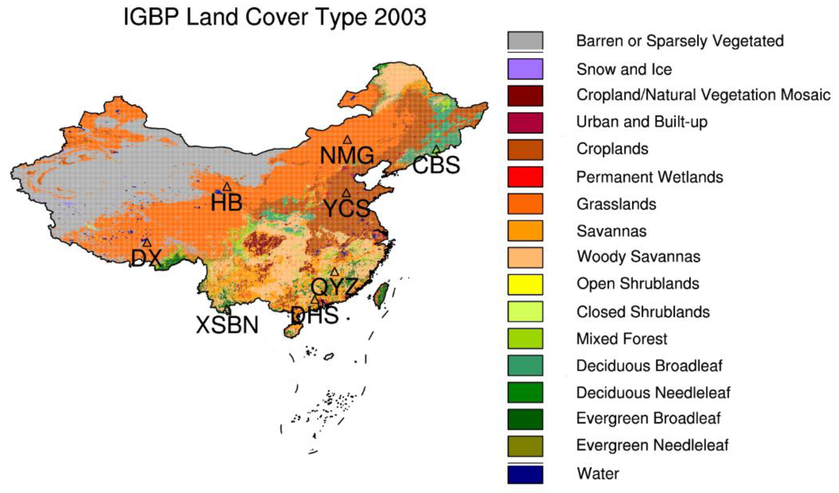
| Sites | Latitude, Longitude, Altitude (°N, °E, m) | IGBP Type | Temp./Precip. (°C/mm) |
|---|---|---|---|
| Changbaishan (CBS) | 41.40, 128.10, 731 | Mixed Forest | 3.6/713 |
| Yucheng Site (YCS) | 36.83, 116.57, 22 | Cropland | 13.1/528 |
| Qianyanzhou (QYZ) | 26.73, 115.07, 100 | Evergreen broad-leaf forest | 18.6/1489 |
| Dinghushan (DHS) | 23.17, 112.54, 100~700 | Evergreen broad-leaf forest | 20.8/1950 |
| Xishuangbannan (XSBN) | 21.92, 101.27, 570 | Evergreen broad-leaf forest | 21.5/1557 |
| Neimenggu (NMG) | 43.63, 116.70, 1100 | Semiarid grassland | 0.96/333.5 |
| Haibei (HB) | 37.61, 101.29, 3250 | Semiarid grassland | −1.7/430 |
| Dangxiong (DX) | 30.47, 91.06, 4286 | Barren/Sparsely vegetated | 1.3/476 |
| Primary Inputs | Data Sources | ||
|---|---|---|---|
| MLSE (Clear and Cloudy) | Norouzi_MLSE (Clear) | Moncet_MLSE (Clear) | |
| Brightness temperature (version, resolution) | AMSR-E/AE_L2A (version 3, Res1 and Res2) | AMSR-E/AE_L2A (version 2, Res1) | AMSR-E/AE_L2A (version 2, Res2) |
| Atmospheric profiles | ECMWF/ERA-20C (37 layers, 0.125°, 3 h) | ISCCP/TOVS (9 layers, 280 km, daily) | NCEP/GDAS (- layers, 1°, 6 h) |
| Skin temperature | ECMWF/ERA-20C (0.125°, 3 h) | ISCCP-DX (30 km, 3 h) | MODIS LST (Instantaneous) |
| Cloud flag | MODIS/MYD06_L2 (Instantaneous) | ISCCP-DX (30 km, 3 h) | MODIS/MYD06_L2 (Instantaneous) |
| Cloud properties | MODIS/MYD06_L2 | / | / |
| Rain flag | AMSR-E/AE_Rain | / | / |
| Month | N | Skin Temperature (K) | 2 m Air Temperature (K) | Near Surface Relative Humidity (%) | |||||||||
|---|---|---|---|---|---|---|---|---|---|---|---|---|---|
| R | RMSE | MB | MAE | R | RMSE | MB | MAE | R | RMSE | MB | MAE | ||
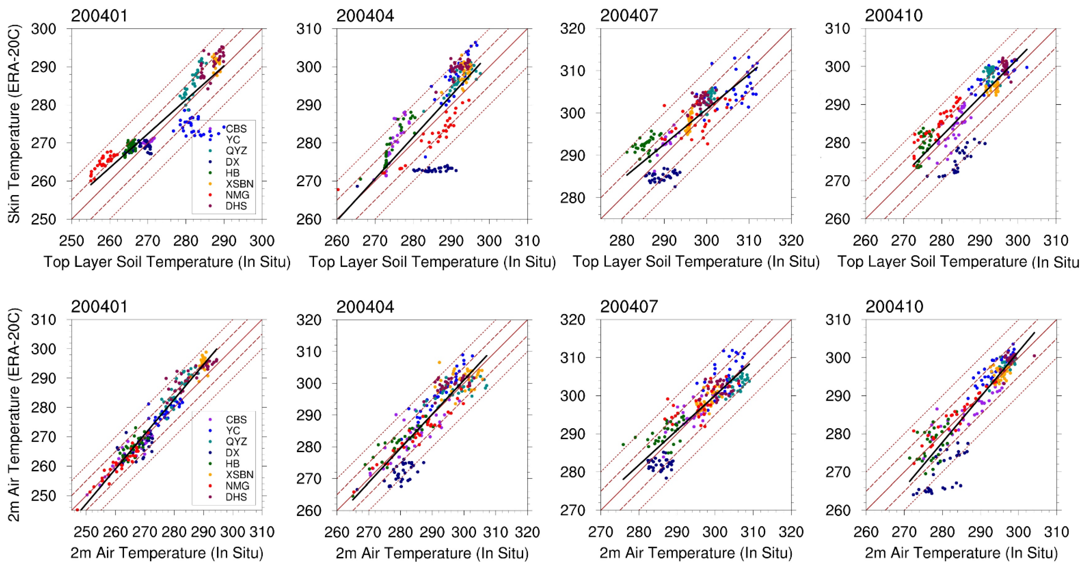
| January, 2004 | 248 | 0.907 | 4.36 | 1.83 | 3.94 | 0.976 | 2.91 | 1.66 | 2.98 | 0.678 | 15.48 | −4.56 | 12.92 |
| April, 2004 | 248 | 0.796 | 6.83 | 2.11 | 6.17 | 0.896 | 5.04 | 0.22 | 4.05 | 0.624 | 17.44 | −4.02 | 16.20 |
| July, 2004 | 248 | 0.822 | 4.01 | 1.58 | 3.77 | 0.886 | 3.57 | 0.41 | 2.87 | 0.593 | 16.02 | −0.83 | 13.57 |
| October, 2004 | 248 | 0.858 | 4.83 | 1.89 | 4.27 | 0.917 | 4.32 | −0.52 | 3.23 | 0.420 | 15.21 | −1.35 | 13.84 |
| Frequency (GHz) | Horizontal Polarizations | Vertical Polarizations | ||||||
|---|---|---|---|---|---|---|---|---|
| 6.925 H | 10.65 H | 18.7 H | 36.5 H | 6.925 V | 10.65 V | 18.7 V | 36.5 V | |
| Samples | 15,796 | 15,796 | 15,796 | 15,796 | 15,796 | 15,796 | 15,796 | 15,796 |
| R | 0.950 | 0.937 | 0.917 | 0.848 | 0.730 | 0.711 | 0.714 | 0.666 |
| RMSE | 0.019 | 0.020 | 0.022 | 0.027 | 0.017 | 0.018 | 0.019 | 0.020 |
| MB | −0.004 | 0.000 | −0.007 | 0.011 | −0.002 | 0.003 | 0.000 | 0.018 |
| MAE | 0.014 | 0.015 | 0.016 | 0.022 | 0.013 | 0.014 | 0.014 | 0.022 |
| Frequency (GHz) | Horizontal Polarizations | Vertical Polarizations | ||||
|---|---|---|---|---|---|---|
| 10.65 H | 18.7 H | 36.5 H | 10.65 V | 18.7 V | 36.5 V | |
| Samples | 15,889 | 15,889 | 15,889 | 15,889 | 15,889 | 15,889 |
| R | 0.939 | 0.936 | 0.935 | 0.852 | 0.840 | 0.838 |
| RMSE | 0.021 | 0.020 | 0.019 | 0.016 | 0.016 | 0.016 |
| MB | 0.011 | 0.004 | 0.013 | 0.010 | 0.004 | 0.013 |
| MAE | 0.016 | 0.014 | 0.017 | 0.014 | 0.013 | 0.016 |
| ChinaFlux Sites | R (MLSE–NDVI) | R (MLSE–Rainfall) | ||||
|---|---|---|---|---|---|---|
| 10.65 H | 18.7 H | 36.5 H | 10.65 H | 18.7 H | 36.5 H | |
| XSBN | 0.64 | 0.51 | 0.35 | −0.24 | −0.32 | −0.43 |
| DHS | 0.45 | 0.32 | 0.15 | 0.37 | 0.25 | 0.12 |
| QYZ | 0.48 | 0.38 | 0.22 | −0.55 | −0.63 | −0.70 |
| CBS | −0.62 | −0.88 | −0.30 | −0.54 | −0.83 | −0.42 |
| YCS | 0.09 | −0.45 | −0.83 | −0.20 | −0.60 | −0.82 |
| NMG | 0.51 | 0.86 | 0.87 | 0.49 | 0.69 | 0.64 |
| HB | −0.52 | −0.53 | −0.49 | −0.78 | −0.78 | −0.68 |
| DX | −0.85 | −0.85 | −0.72 | −0.94 | −0.93 | −0.80 |
Publisher’s Note: MDPI stays neutral with regard to jurisdictional claims in published maps and institutional affiliations. |
© 2021 by the authors. Licensee MDPI, Basel, Switzerland. This article is an open access article distributed under the terms and conditions of the Creative Commons Attribution (CC BY) license (https://creativecommons.org/licenses/by/4.0/).
Share and Cite
Hu, J.; Fu, Y.; Zhang, P.; Min, Q.; Gao, Z.; Wu, S.; Li, R. Satellite Retrieval of Microwave Land Surface Emissivity under Clear and Cloudy Skies in China Using Observations from AMSR-E and MODIS. Remote Sens. 2021, 13, 3980. https://doi.org/10.3390/rs13193980
Hu J, Fu Y, Zhang P, Min Q, Gao Z, Wu S, Li R. Satellite Retrieval of Microwave Land Surface Emissivity under Clear and Cloudy Skies in China Using Observations from AMSR-E and MODIS. Remote Sensing. 2021; 13(19):3980. https://doi.org/10.3390/rs13193980
Chicago/Turabian StyleHu, Jiheng, Yuyun Fu, Peng Zhang, Qilong Min, Zongting Gao, Shengli Wu, and Rui Li. 2021. "Satellite Retrieval of Microwave Land Surface Emissivity under Clear and Cloudy Skies in China Using Observations from AMSR-E and MODIS" Remote Sensing 13, no. 19: 3980. https://doi.org/10.3390/rs13193980