Climate Effects on Vertical Forest Phenology of Fagus sylvatica L., Sensed by Sentinel-2, Time Lapse Camera, and Visual Ground Observations

Abstract

Contemporary climate change leads to earlier spring phenological events in Europe. In forests, in which overstory strongly regulates the microclimate beneath, it is not clear if further change equally shifts the timing of leaf unfolding for the over- and understory of main deciduous forest species, such as Fagus sylvatica L. (European beech). Furthermore, it is not known yet how this vertical phenological (mis)match—the phenological difference between overstory and understory—affects the remotely sensed satellite signal. To investigate this, we disentangled the start of season (SOS) of overstory F.sylvatica foliage from understory F. sylvatica foliage in forests, within nine quadrants of 5.8 × 5.8 km, stratified over a temperature gradient of 2.5 °C in Bavaria, southeast Germany, in the spring seasons of 2019 and 2020 using time lapse cameras and visual ground observations. We explained SOS dates and vertical phenological (mis)match by canopy temperature and compared these to Sentinel-2 derived SOS in response to canopy temperature. We found that overstory SOS advanced with higher mean April canopy temperature (visual ground observations: −2.86 days per °C; cameras: −2.57 days per °C). However, understory SOS was not significantly affected by canopy temperature. This led to an increase of vertical phenological mismatch with increased canopy temperature (visual ground observations: +3.90 days per °C; cameras: +2.52 days per °C). These results matched Sentinel-2-derived SOS responses, as pixels of higher canopy height advanced more by increased canopy temperature than pixels of lower canopy height. The results may indicate that, with further climate change, spring phenology of F. sylvatica overstory will advance more than F. sylvatica understory, leading to increased vertical phenological mismatch in temperate deciduous forests. This may have major ecological effects, but also methodological consequences for the field of remote sensing, as what the signal senses highly depends on the pixel mean canopy height and the vertical (mis)match.

1. Introduction

Contemporary climate change leads to earlier spring phenological events in Europe, such as bud burst and leaf unfolding of trees, with an average rate of −2.5 days per °C warming [1]. These phenological shifts can have massive effects, ranging from the fitness of individuals to the whole ecosystem. At the individual level, leaf unfolding of trees too early can lead to an increase of damage by late-frost events in spring, e.g., [2,3]. At the ecosystem level, phenological shifts of vegetation can result in or increase mismatches with individuals in higher trophic levels, which are often not equally sensitive to climate change and therefore shift at dissimilar rates, e.g., [4,5,6,7,8]. Mismatches can also occur non-trophically within the level of primary producers. In forests, early canopy closure in spring will provoke too low light levels beneath the overstory, creating more unsuitable growing conditions for understory vegetation [9,10]. To buffer these different types of mismatches, land use planning and forest management could play a key role, e.g., by promoting larger proportions of vegetation that is less sensitive to climate change, or by increasing spatial phenological variability [5,11].

Previous studies have mainly focused on horizontal phenological variability, e.g., [11,12,13], although some studied elevational gradients on the landscape scale [14,15]. However, especially on the scale of a forest with multiple vertical layers of primary productivity, it is important to acknowledge that space has not two but three dimensions [10,16]. Considering a forest as a 2D-feature, by doing observations on only one random layer or the integrated vertical column from above and generalizing them to the whole vertical dimension, could introduce biased conclusions on the habitat of animals, as they are often stratified to only one specific forest layer [17]. Furthermore, for the primary producers themselves, studying phenology three-dimensionally is of high importance, as the future of the forest overstory is dependent on the fitness of tree regeneration in the understory [18], and, in that way, it can highly impact the carbon balance.

Previous studies showed that both among and within species, understory ephemerals, shrubs, and tree juveniles generally reach budburst and leaf unfolding earlier in spring than adult trees in the overstory [19,20,21,22]. This pattern, which is determined ontogenetically [21], is of high importance for tree populations since photosynthetically active radiation (PAR) at the forest floor is drastically reduced after overstory flushing [23,24]. Gill et al. [23] found that, in a beech-maple dominated hardwood forest, the transmission of PAR from the canopy top to 1 m above the forest floor was reduced from 55% before overstory budburst to 1–2% after full leaf unfolding of the overstory and that understory CO₂ gains per time unit before overstory budburst was significantly higher than afterwards. Jolly et al. [25] also found that the productivity of the understory is highly dependent on its timing of leaf flushing and senescence, relative to that of the overstory, as they found that an extension of the understory’s growing season, relative to that of the overstory, by one week led to an increase in productivity of 32% and an extension of two weeks, even to an increase of 55%. Despite higher probabilities of late-frost risks with earlier leaf flushing, the net survival rate of understory individuals that leaf out earlier are expected to increase, as Jones et al. [26] and Seiwa et al. [27] found for seedlings of Acer rubrum and Acer mono, respectively.

However, it would be an oversimplification of reality to assume that this ontogenetically determined earlier understory flushing relative to the overstory is a static phenomenon, as there are reasons to expect interaction effects between climate and vertical forest gradients to explain spring phenology. Forest canopies are able to create microclimates underneath, with the temperature and radiation in the understory fluctuating less than in the overstory [10,28]. In this way, the climate change effects are buffered in the understory. Jolly et al. [25] suggested that altered matches between overstory and understory phenology induced by climate warming can affect stand structure and productivity in the long term. Heberling et al. [9] showed that the spring phenology of understory wildflowers responded less to warming than the trees in the overstory above, and, in that way, their study was the first to show that non-trophical phenological (mis)matches between understory and overstory are expected to alter with climate change. It is not known yet if this also applies to tree regeneration of deciduous species native to temperate forests, such as Fagus sylvatica L. (European beech), the main deciduous tree species in Central and Western Europe, and of high ecological and economical importance [29]. Thus, understanding how well its understory is able to keep “phenologically escaping” [30] with ongoing climate change is very important, as it will be the future overstory. It will be economically relevant to wood production and ecologically relevant by providing a habitat to many animal species [10,18]. Next to that, tree regeneration is expected to have a narrower range of adaptation strategies than the herbaceous part of the understory, as the first is usually less species rich. Therefore, tree regeneration might be more vulnerable to variables associated with climate change than the herbaceous understory studied by Heberling et al. [9]. A recent study of Vitasse et al. [31] reported delayed budburst of tree seedlings from several species, including F. sylvatica, under artificial shading nets that intercepted 70% of incoming radiation and were causing a cooler microclimate at the same time. We assume that an early closing forest canopy can have the same effect, but investigation is required.

As variation in global radiation is known to affect local temperature reasonably [32], and furthermore might also directly affect leaf phenology of F. sylvatica [31], topography and cloud cover based global radiation can also be a very important variable to downscale coarsely gridded air temperature. Therefore, next to global radiation and air temperature, a variable based on a combination of both, which would be called “surface temperature”, or—especially in forests with a large vertical climatic gradient—“canopy temperature” [32], would be expected to maximally expose differences between the overstory and understory.

Scaling up from the level of individuals to stands, forests, and even landscapes, multispectral satellite remote sensing has accelerated the study of phenology immensely by covering larger spatial and temporal extents and its lower degree of subjectivity compared to visual in-situ ground observations, with the earliest studies done by Myneni et al. [33] and White et al. [34]. Therefore, a very important second knowledge gap is how shifting vertical forest phenology patterns will influence the interpretation of data by multispectral satellite remote sensing. Among the latter, products provided by the European Space Agency’s (ESA) Sentinel-2 are well appreciated by the research community due to the high spatial resolution (10 m), global coverage, and free public access.

An important drawback of Sentinel-2, and satellite remote sensing in general, in the study of the phenology of forests is that it looks at the canopy solely from above [35,36,37,38]. For deciduous forests, this means that in the part of the year in which the overstory leaves have flushed and form a closed canopy, the forest layers beneath the overstory are partly or completely absent from the signal, whereas in the part of the year in which the upper part of the canopy is not yet closed, an integrated signal is sensed from the forest floor to the top of the canopy, e.g., [38]. However, without additional phenological measurements from visual in situ ground observations or cameras, the relative contribution of each layer to the signal at different points in time is unknown [38,39]. Given the generally accepted assumption that understory flushes before overstory [20], results of Ahl et al. [35] and Ryu et al. [38] indicated that, in the time period before overstory canopy closure, it is mainly the signal from the forest understory that is sensed. Ahl et al. [35] found that the MODIS signal predicted spring phenology weeks in advance of overstory observations from the ground. Ryu et al. [38] found the MODIS signal to be much more correlated with visual in situ ground observations from the understory than those from the overstory. Elaborating on this, Pisek et al. [40] and Tuanmu et al. [37] were able to successfully disentangle remotely sensed understory phenology from overstory phenology purely based on MODIS data. Nevertheless, the forests in both studies were very specific. In the study of Tuanmu et al. [37], the understory (evergreen bamboo shrubs) was very clear and spectrally and phenologically different from the overstory (deciduous, evergreen or a mix of tree species). In the study of Pisek et al. [40] on semiarid to boreal forests, overstory vegetation was rather sparse. Temperate deciduous forests are often dense, meaning phenological disentangling will hardly be possible [39], and, adding to that, the understory may consist of the same species as the overstory and therefore have a more similar phenology. Although Misra et al. [41] showed that LIDAR-derived stand structure data helped to explain spatial variability in “land surface phenology”, they did not disentangle the phenology of specific forest layers.

Furthermore, when the time gap between overstory and understory is not static, but instead, as we hypothesized, is rather susceptive to climate change, we can argue that the layer that is actually sensed is dependent on the phenology of the understory relative to the overstory and on the density of the overstory covering the understory. Due to the fact that the vertical integration of the understory is of an unknown proportion (before canopy closure), or absent (after canopy closure) in the remotely sensed signal, we argue that it is impossible to generalize climate change effects on either overstory, understory, or temperate deciduous forest phenology as a whole, solely based on satellite remote sensing techniques.

Therefore, to disentangle overstory from understory, a combination with other sensors, such as time lapse cameras and/or visual in situ ground observations, is required. In several studies, a combination of methods was used to study vegetation phenology, e.g., [22,38,42,43,44,45,46,47,48,49], which showed the possibilities of combining and partly replacing the classical visual in situ ground observations with more quantitative (satellite and camera observations), higher spatial coverage (satellite), and higher temporal resolution (cameras) methods. Derivatives to define phenological metrics, such as the start of the season (SOS), are found to align well with each other and are given ecological meaning. Nevertheless, only some of these studies disentangled the phenology of overstory and understory [38,49], although we see this as a key advantage of ground and camera observations, and essential to do in forests, as the vertical dimension is inevitable. Furthermore, most of these studies are purely methodical and were conducted over single years or seasons and single sites or areas, and thus the effects of climate variability were not tested.

Here we aimed to investigate the following research questions: (1) how do the phenology of F. sylvatica overstory and understory, and the associated vertical (mis)match, respond to the main environmental variables associated with climate change, by using visual in situ observations from the ground and time lapse cameras, and (2) what does this mean for the sensed SOS signal by Sentinel-2.

2. Materials and Methods

2.1. Study Design

In the spring seasons of 2019 and 2020, we observed the phenology of F. sylvatica in deciduous and mixed temperate forests in nine 5.8 × 5.8 km quadrants within the federal state of Bavaria, southeast Germany (Figure 1;

Table 1. Description of the nine study quadrants (5.8 × 5.8 km), including their center coordinates, elevation, mean annual temperature (1981–2010), mean annual precipitation (1981–2010), as well as the number of samples per method. Note that all samples were taken in two years (2019 and 2020). Camera sites always included one camera facing understory and one camera facing overstory. Abbreviations: temperature (temp.), precipitation (precip.), overstory (over.), understory (under.), individuals (indivs.). “Ground” stands for ground-based visual phenological observations.

Quadrant	Center Coordinates (°E, °N)	Elevation (m)	Mean Annual Temp. (°C)	Mean Annual Precip. (mm)	Camera Sites (Section 2.1)	Groundover. Indivs. (Section 2.2)	Ground Under. Indivs. (Section 2.2)	Sentinel-2 Indivs. (Section 2.5.2 Dataset 1)	Sentinel-2 Pixels (Section 2.5.2 Dataset 2)
Q1	9.77, 49.76	294	9.2	635	3	3	1	4	12,356
Q2	9.94, 49.89	309	9.1	678	2	3	1	20	15,923
Q3	10.44, 50.07	328	8.8	701	-	3	2	8	-
Q4	11.75, 48.92	449	8.6	675	3	4	3	11	15,384
Q5	11.85, 48.58	490	8.4	650	-	3	3	13	132
Q6	10.53, 49.92	412	8.2	809	-	3	3	12	17,029
Q7	11.70, 49.13	543	7.9	785	2	4	3	8	3614
Q8	13.36, 48.78	491	7.8	1215	1	3	3	10	3910
Q9	13.54, 48.88	785	6.8	1367	2	3	3	6	-
Total					13	29	22	92	68,348

). This administrative unit forms a central and representative part of the geographical range of F. sylvatica and is therefore an ideal study area. These quadrants are a subset of the 60 quadrants of the stratified study design developed by Redlich et al. [50] and are based on existing grid cells of ‘TK 25’ (topographical maps, scale 1:25,000), allowing for the comparison with other long-term monitored ecological data. The nine quadrants used here were chosen over a mean annual temperature gradient over 30 years (1981–2010) from 6.78 °C (Q9) to 9.24 °C (Q1). Three different methods were used to observe phenology: time lapse cameras, visual in situ ground observations, and Sentinel-2 imagery.

2.2. Hourly Time Lapse Camera Images

2.2.1. Sampling

We selected up to three locations per quadrant to place two Cuddeback C2 wildlife cameras with a time lapse function in March 2019, when all F. sylvatica buds were still closed and no other vegetation was blocking the view. One of them was installed at a height of ~70 cm and facing F. sylvatica foliage in the understory, which we defined as the lowest 2 m of the forest, in line with the definition of understory by Gressler et al. [51]. In that way, understory was potentially forageable by hoofed animals, such as roe deer, an important ecological determinant of European and, in particular, Bavarian forests, e.g., [52,53,54]. The other camera was installed at a height of ~3 m and positioned diagonally upwards facing the overstory of F. sylvatica foliage, as Ryu et al. [38] did in their study. Cameras took one picture per hour between sunrise and sunset, with “aspect” set to “full” and “zone” to “wide”. We set the image size (“Lapse SZ”) to 5 megapixels (MP), as this resulted in sufficient quality for both visual and quantitative analysis, while saving storage space, as compared to the option of 20 MP.

All cameras were operational until August 2020. Batteries were replaced and SD cards read out every three months. For analysis, we selected only complete time series from sites that had, for both spring seasons, unmixed F. sylvatica foliage recorded for the overstory and the understory during the greenup period, roughly between day of the year (DOY) 95 and DOY 125. This resulted in 13 sites, spread out over six quadrants (Q1, Q2, Q4, Q7, Q8, and Q9), all having an understory 2019, overstory 2019, understory 2020, and overstory 2020 spring time series of F. sylvatica (Table 1).

2.2.2. Pre-Processing

For the images in those time series, we drew expert-based regions of interest (ROI) in which only F. sylvatica foliage occurred and was not disturbed by other features, such as moving branches in the foreground, through time. Subsequently, we selected the images taken between 10:00 a.m. and 2:00 p.m., and between DOY 80 and 140. Per image, we calculated the mean green chromatic coordinate (GCC) of all pixels within the ROI on each time step as a measure of the standardized greenness, e.g., [44,48,55] via:

$$GCC=\frac{G}{R+G+B}$$

(1)

where R, G, and B are the mean red, green and blue digital numbers, respectively. This resulted in a time series of four GCC values per DOY. To compare cameras and years, we normalized these data, similar to how Richardson et al. [56] did, by setting the mean GCC from images taken between DOY 80 and DOY 95, in which all F. sylvatica buds were closed, to 0, and the mean GCC from images taken between DOY 125 and DOY 140, in which all F. sylvatica leaves were at mature size, to 1, by which the values in between were stretched accordingly. As weather conditions are known to potentially affect the camera signal [55], we applied a filter by taking the 60th percentile of a 3 day moving window, and a time step of 1 day, as the proposed 90th percentile by Sonnentag et al. [55] resulted in systematically too high GCC values, compared to the unfiltered data. Subsequently, we fitted a double-logistic function to each time series, according to Beck et al. [57], which automatically filtered out too low winter values, and thus was particularly useful in the temporally dense time series. Then, the start of season (SOS) was derived by taking the DOY at which a normalized GCC of 0.5 was reached for the modelled values. We chose this threshold since the increase in both springs was very steep (increase in normalized GCC from 0 to 1, mostly in ~<7 days) and on average the steepest increase in greenness tended to occur at this threshold (similar to the reasoning of Richardson et al. [56] for their threshold choice). For both drawing ROIs as well as fitting double-logistic curves, we used the phenopix package [58] in R [59]. The camera-derived normalized GCC time series for one quadrant (Q4), as an example, is presented in Figure A1 in Appendix A.

We derived “vertical mismatch” between overstory and understory by subtracting overstory SOS from understory SOS per site [9]. Thus, negative values represent the number of days the understory was flushing before the overstory (“phenologically escaping”) [30], which is the classical pattern. Positive values represent the number of days the overstory was flushing before understory, meaning an inverted classical pattern.

2.3. Ground Observations

2.3.1. Sampling

Visual in situ ground observations were performed (further referred to as “ground observations”). Within each quadrant, we selected one deciduous or mixed forest stand in which F. sylvatica was one of the dominant species. In each forest stand, we selected at least three F. sylvatica overstory and three F. sylvatica understory individuals. We defined an overstory individual as being part of the upper canopy layer, either by being a dominant, codominant, subdominant, or suppressed tree [60], with a minimum height of 15 m, by which the definition of overstory as defined by Gressler et al. [51] was slightly extended. We defined understory individuals as individuals of <2 m high, in accordance with the camera observations and Gressler et al. [51]. From these individuals, we near-weekly estimated the percentage of buds per individual that had burst (“budburst”) and the percentage of leaves that were fully out (“leafout”), starting from before budburst until when all leaves were completely unfolded. “Budburst” was neglected for further analysis, as it was often hard to identify in tree crowns despite the use of binoculars. We defined “leafout” as the moment at which the leaf was completely visible, all the way to the petiole, in accordance with the BBCH 11 (Biologische Bundesanstalt, Bundessortenamt und Chemische Industrie) [61]. For further analysis, we only used the individuals measured in both years, resulting in a total of 29 overstory individuals and 22 understory individuals spread over the nine quadrants (Table 1).

2.3.2. Pre-Processing

We used the phenex package [62] in R [59] to fit a double-logistic function to each time series for leafout ranging from 0% to 100%, as per Fischer [63]. Then, we derived “leafout 50%” as the DOY at which the modelled values reached 50%, as this implied that the majority of leaves were unfolded and, furthermore, we estimated that, at this threshold, the average curve incline was highest (similar to Richardson et al. [56]). We defined leafout 50% as SOS, to compare with remotely sensed phenological derivatives ([64], see Section 2.5.2). To illustrate this, all leafout fraction time series derived from ground observations for one quadrant (Q4) are presented in Figure A2.

We derived a value of “vertical mismatch” for each quadrant × year by subtracting the mean SOS of the overstory individuals from the mean SOS of the understory individuals.

2.4. UAV Data

In order to link ground observations (Section 2.3) to satellite remote sensing (Section 2.5), we made use of a UAV to identify tree crowns in the field. Between 5 and 8 May 2020, when the leaves of the majority of the deciduous trees in all quadrants were out, but species were most distinguishable because of different shades of visual green, we executed UAV flights over each of the nine forest stands using a DJI P4 Multispectral, which had a separate camera, to take high quality RGB-images with a spatial resolution of ~5 cm at an acquisition height of 100 m. These images were geo-referenced with a precision of ~10 cm and were stitched together to form an orthomosaic (GeoTiff) using Pix4DMapper 4.5.

2.5. Sentinel-2 Data

2.5.1. Data Retrieval

Using the Sen2R package [65] in R [59], we downloaded all available cloud-free Sentinel-2 level-2A tiles from 20 February to 30 June for 2019 and 2020 for the spatial extent of the nine quadrants. This product contains bottom-of-atmosphere (BOA) reflectance of 13 spectral bands, from which the visual and near-infrared bands have a spatial resolution of 10 m. Using the same package, and based on a scene classification included in the level-2A product, we filtered out pixels classified as “cloud (high probability)”, “cloud (medium probability)”, “thin cirrus”, “snow”, “cloud shadows”, “unclassified”, “saturated or defective”, and “no data”.

2.5.2. Pre-Processing

Using multispectral remote sensing, the greenness or productivity of vegetation can be defined as a certain ratio between reflectance in the near-infrared and the red band [66], and, in that way, it can measure seasonal vegetation development over time [33]. Here we used the normalized difference vegetation index (NDVI), which we calculated for each non-cloud covered pixel in each quadrant-clipped Sentinel-2-tile by:

$$NDVI=\frac{N-R}{N+R}$$

(2)

where N and R are the reflectances in the near-infrared and the red band, respectively.

Subsequently, two data sets were used as input for Sentinel-2 analysis:

• Data set 1 was generated for the forest stands in which ground observations were also conducted. There, we selected the individuals we did ground observations for, and, additionally, we selected two more random locations per forest stand, selecting all F. sylvatica individuals that fell in an angle-count sample as was done by the German forest inventory “Bundeswaldinventur” [67]. This resulted in a total of 92 trees spread out over the nine quadrants (Table 1). We imported the UAV-acquired RGB orthophotos as a tile layer in ESRI ArcGIS Online, which we enabled for offline use. Then, using the ESRI ArcGIS Collector application on a tablet in the field, we identified all 92 selected trees (ground phenology + additional individuals) on the orthophoto tile layer and manually drew the polygons of the crowns from the selected trees in a separate layer. After this, we extracted the NDVI for each crown at each DOY that had an acquired cloud-free Sentinel-2 image, using bilinear interpolation among the cells where each crown overlapped.
• Data set 2 was generated for quadrant-wide beech forests. We masked the quadrant-wide cloud-free Sentinel-2 NDVI time series by a shapefile, including all forests owned by the Bavarian State Forest agency in the quadrant in which F. sylvatica was the dominant species, according to the Bavarian State Forest agency. This forest type was present in 7 out of the 9 quadrants.

For both Sentinel-2 data sets 1 and 2, we used the phenex package [62] to fit a double-logistic function to the NDVI time series of each individual crown (data set 1) or pixel (data set 2) for both years. Modelled values were normalized from 0 to 1, with the lowest modelled value set to 0 and the highest set to 1. We defined the start of season (SOS) as the DOY in which a curve reached a threshold of 0.3. Although the literature was not uniform in terms of which greenness threshold best represented field-observed phenological events, such as leafout, and as this can vary depending on the spatial resolution of the satellite product [68], we chose a threshold of 0.3 since, according to White et al. [64], Landsat TM (30 m resolution)-derived SOS based on a threshold of 0.3 best represented the moment at which the “plot average reached full leafout”, which corresponds to our “leafout 50%” on the tree level. Equally, following Misra et al. [69], MODIS (231.65 m resolution)-derived SOS was based on a threshold of 0.2, which matched best with ground-observed understory phenology, and a threshold of 0.5 for the leaf unfolding of deciduous trees. We filtered out pixels or trees that did not greenup in a temporally dense acquisition period, and those from which the difference between summer and winter normalized NDVI, i.e., the amplitude, was lower than 0.2. We additionally removed pixels or trees with an unrealistically late (after DOY 125) or early (before DOY 100) start of season. For further analysis, we only used trees and pixels present in both years after filtering. All normalized NDVI time series derived from Sentinel-2, data set 1, for one quadrant (Q4) are presented in Figure A3.

2.6. Environmental Variables

2.6.1. Tree and Canopy Height

We measured the height of all selected trees (Section 2.5.2, data set 1) individually. A Vertex IV (Haglöf Sweden) was used for trees > 3 m and a meter stick for trees < 3 m. We further refer to this variable as “tree height”.

In order to derive “canopy height” for the selected pixels (Section 2.5.2, data set 2), we retrieved a digital surface model (DSM) in LAS format, with a spatial resolution of 40 cm in a radius of 700 m around each ground-observed forest and each camera site, which was derived by the Bavarian “Landesamt für Digitalisierung, Breitband und Vermessung” (LDBV) on the basis of aerial images, acquired in either summer 2019 or summer 2020. Secondly, we also retrieved a digital terrain model (DTM) from the LDBV in tiff-format, which was acquired by laser scanning from an air plane (LIDAR) with a spatial resolution of 5 m for the same area. We calculated “canopy height” at a spatial resolution of 1 m by subtracting the DTM from the DSM, using the lidR package [70] in R [59].

2.6.2. Air Temperature

As the main driver of plant phenology [1], we obtained monthly averaged mean daily air temperature (°C) by retrieving 1 × 1 km gridded monthly temperature data from the German Meteorological Service (Deutsche Wetterdienst, DWD) [71].

2.6.3. Global Radiation

Using the area solar radiation function from the spatial analyst toolbox within ArcGIS Pro 2.6.0, we calculated spatially and temporally explicit global radiation in watt hours per square meter (Wh/m²) for each 5 m grid cell based on the DTM, using methods described by Fu et al. [72] (see also Allen et al. [73] for more details on the method). With the DTM as input, this area solar radiation tool accounts for topography including slope, aspect, sun-earth geometry, and sky obstruction by topographic features. It likewise accounts for atmospheric conditions by including the diffuse proportion and the transmittivity as input [72]. To calculate the diffuse proportion and transmittivity, we used SEVIRI/AVHRR-derived daily fractional cloud cover (CFC), which we retrieved from EU-METSAT’s Satellite Application Facility on Climate Monitoring (CM SAF), with a spatial resolution of 15 × 15 km, as per the method described by Huang et al. [74]. Afterwards, by dividing the global radiation over the number of hours per month, we derived the mean global radiation in W/m² per month.

2.6.4. Canopy Temperature

We included topography-based global radiation to downscale gridded air temperature. As it was empirically derived for a Festuca ovina grassland by Bennie et al. [32], we calculated canopy temperature (temperature directly at the canopy surface) (Tc) using:

$$Tc=Tg+0.013 Rad$$

(3)

where Tg is gridded air temperature (°C) and Rad is global radiation (W/m²). We assumed that wind speed was mainly >1 m/s, a similar albedo between F. sylvatica and F. ovina, neglected the temperature difference potentially caused by tree height, did not account for canopy structure, nor for differences in transpiration rates. The coefficient of +0.013 was also in line with Ashcroft [75], who empirically modelled a parameter of +0.01327 to multiply with radiation (W/m²) to retrieve a maximum temperature.

We extracted monthly means of air temperature, global radiation, and canopy temperature for: (a) all Sentinel-2 and ground observed tree polygons, and (b) a radius of 50 m around all camera sites using bilinear interpolation. For further analysis, only the month of April was used, as preliminary results showed that air temperature of this month explained ground-, camera-, and Sentinel-2 phenology better than any other single month or a combination of months. Furthermore, we only presented the results for canopy temperature here, since similar results were obtained for all three explanatory variables. Canopy temperature was preferred over air temperature and global radiation, since it integrates the other two ones (see Equation (3)), is spatially more explicit, and most directly affects vegetation.

2.7. Statistical Analysis

To test differences between 2019 and 2020 in terms of the climate variables in the forest stands for which we did ground- and Sentinel-2 observations, we used paired t-tests with the quadrants as pairs.

To test differences in SOS per layer between 2019 and 2020 and per year between layers, we ran generalized linear mixed-effects models (GLMM), accounting for grouping by quadrant and site (for cameras) and quadrant and individual (for ground observations) by including them as random factors, using the lme4 package [76] in R [59]. To test differences in Sentinel-2 SOS between 2019 and 2020, we also performed GLMMs with quadrant and individual as random factors.

To test the linear relation between overstory SOS and the vertical mismatch with the understory, we used separate GLMMs for both camera and ground observations, with the overstory SOS as the fixed effect, the vertical mismatch as the dependent variable, with quadrant and site (for cameras) or only quadrant (for ground observations as the random factors.

To test the linear effects of canopy temperature on SOS for all cameras and ground observations, we first centered canopy temperature to its mean. Then, we ran GLMMs with the canopy temperature as a fixed effect to predict the SOS of the overstory, the SOS of the understory, and on vertical mismatch per site (for cameras) or per individual (for ground), all in separate models, with quadrant and site (for cameras) or quadrant and tree individual (for ground observations) as the random factors. For Sentinel-2, we ran a GLMM to test the effect of canopy temperature on SOS of the tree polygons. To test if the canopy temperature effect differed with tree height, we also included tree height (m) per individual in the Sentinel-2 model and the interaction between tree height and canopy temperature. Quadrant and tree individual were used as random effects.

Lastly, to deepen our insight into the relation between canopy height and spring phenology, as obtained by Sentinel-2, for the pixels in the state forests dominated by F. sylvatica (see Section 2.5 analysis 2), we tested the effect of mean canopy height per Sentinel-2 pixel area, further referred to as “pixel mean canopy height”, on the SOS using simple linear models per quadrant per year and compared results between the two years.

For the analyses we additionally used the raster package [77], RStoolbox package [78], the jpeg package [79], and the lubridate package [80]. For visualizations, we used the ggplot2 package [81] and the cowplot package [82] in R [59].

3. Results

In 2020, over all quadrants, mean April global radiation (206.01 W/m²) was 22.50 W/m² higher than in 2019. Similarly, in 2020, the mean April air temperature (13.16 °C) was 0.68 °C higher than in 2019, and in 2020, the mean April canopy temperature (10.48 °C) was 0.97 °C higher than in 2019.

Comparing the years using the Sentinel-2 observations, the pixels overlapping with polygons around overstory individuals reached SOS in 2020 on DOY 108.13, which was 2.57 days earlier than in 2019 (p < 0.001). Furthermore, for each individual in every quadrant, SOS was earlier in 2020 than in 2019 (Figure 2a,b).

Comparing years per layer for the ground observations, the overstory reached SOS in 2020 on DOY 109.00, which was 3.46 days earlier than in 2019 (p < 0.001), while the understory reached SOS in 2020 on DOY 112.28, which was 1.2 days later than in 2019 (p = 0.09). Comparing layers per year for the ground observations, the understory reached SOS in 2019 on DOY 111.20, which was 1.20 days earlier than the overstory, although not significant (p = 0.38), while in 2020, the understory reached SOS on DOY 112.93, which was 3.84 days later than the overstory (p < 0.001) (Figure 2c,d).

Comparing years per layer for the camera observations, the overstory reached SOS on DOY 109.95, which was 3.38 days earlier in 2020 than in 2019 (p < 0.001), while the understory SOS on DOY 111.51 was not significantly different from 2019 (0.10 days later, p = 0.79). Comparing layers per year for the camera observations, the understory reached SOS in 2019 on DOY 111.37, which was 1.96 days earlier than the overstory (p = 0.007), while, in 2020, the understory SOS was reached on DOY 111.47, 1.52 days later than the overstory, although not significant (p = 0.13) (Figure 2e,f). Furthermore, comparing all single sites (Figure 2e), we saw that the overstory advance in 2020, as compared to 2019, was always larger than the understory advance, which was sometimes even delayed. In other words, the vertical mismatch between the overstory and understory was higher at all sites in 2020 compared to 2019.

We found a negative relation between the SOS of the overstory and the vertical mismatch with the understory (Figure 3). This trend was consistent across methods. For camera observations, we found an increased mismatch with the understory of 0.93 days per day of overstory advancing (p < 0.001), indicating hardly any advancing of the understory SOS when the overstory SOS was advancing. For ground observations, we found an increased vertical mismatch with the understory of 1.31 days for an advance of the overstory of 1 day (p < 0.001), indicating an understory SOS that was delayed when the overstory SOS was advancing.

Figure 4 and

Table 2. Results of seven separate GLMMs (rows) explaining SOS per layer or vertical mismatch between overstory and understory. Each row represents one model, with the dependent variable listed in the first column, followed by the method in the second column. The third column represents the centered fixed effect. For camera and visual ground observations, that was always canopy temperature (CT). For Sentinel-2 observations, the one model had CT, tree height, and the interaction between CT and tree height (CT × height) as fixed effects. The coefficients represent regression slopes of the fixed effects explaining the dependent variables. Since CT and height are both centered to their means, their centered intercepts are listed for the different models. “n” represents number of trees (see Table 1) × 2 years (for Sentinel-2 and visual ground observations) or number of sites × 2 years (for camera observations). Which random effects are used per model is described in the methods. Stars indicate significance.

Dependent Variable	Method	Fixed Effect	Coefficient			Centered Intercept	n
Models Camera and Visual Ground Observations
SOS overstory (DOY)	Camera	CT	−2.574 ***			111.494 ***	26
SOS overstory (DOY)	Ground	CT	−2.860 ***			110.705 ***	58
SOS understory (DOY)	Camera	CT	−0.175			111.450 ***	26
SOS understory (DOY)	Ground	CT	+0.644			111.632 ***	44
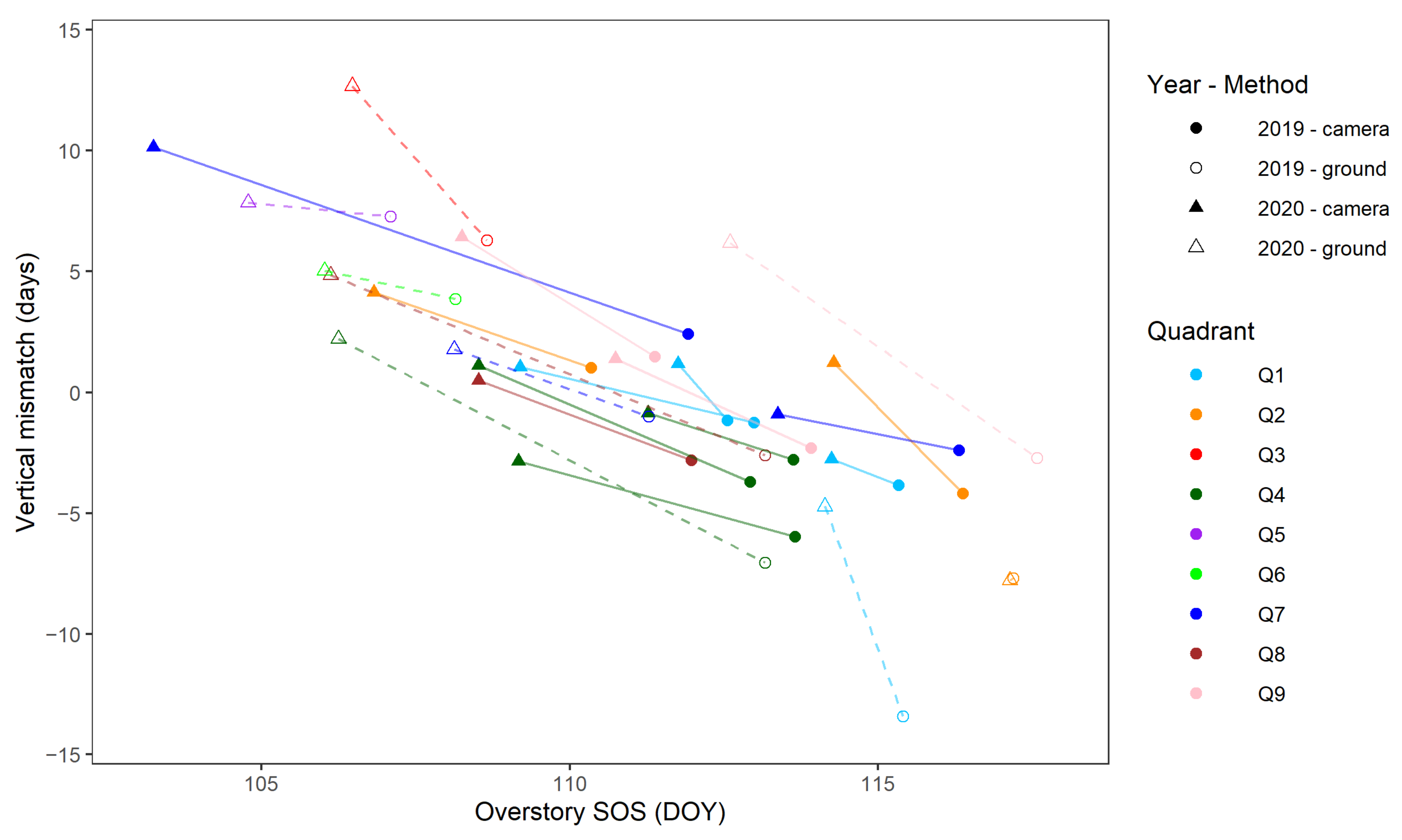
Vertical mismatch (days)	Camera	CT	+2.522 ***			0.072	26
Vertical mismatch (days)	Ground	CT	+3.901 **			0.085	18
Models Sentinel-2 Observations
			CT coefficient	Height coefficient	Interaction coefficient
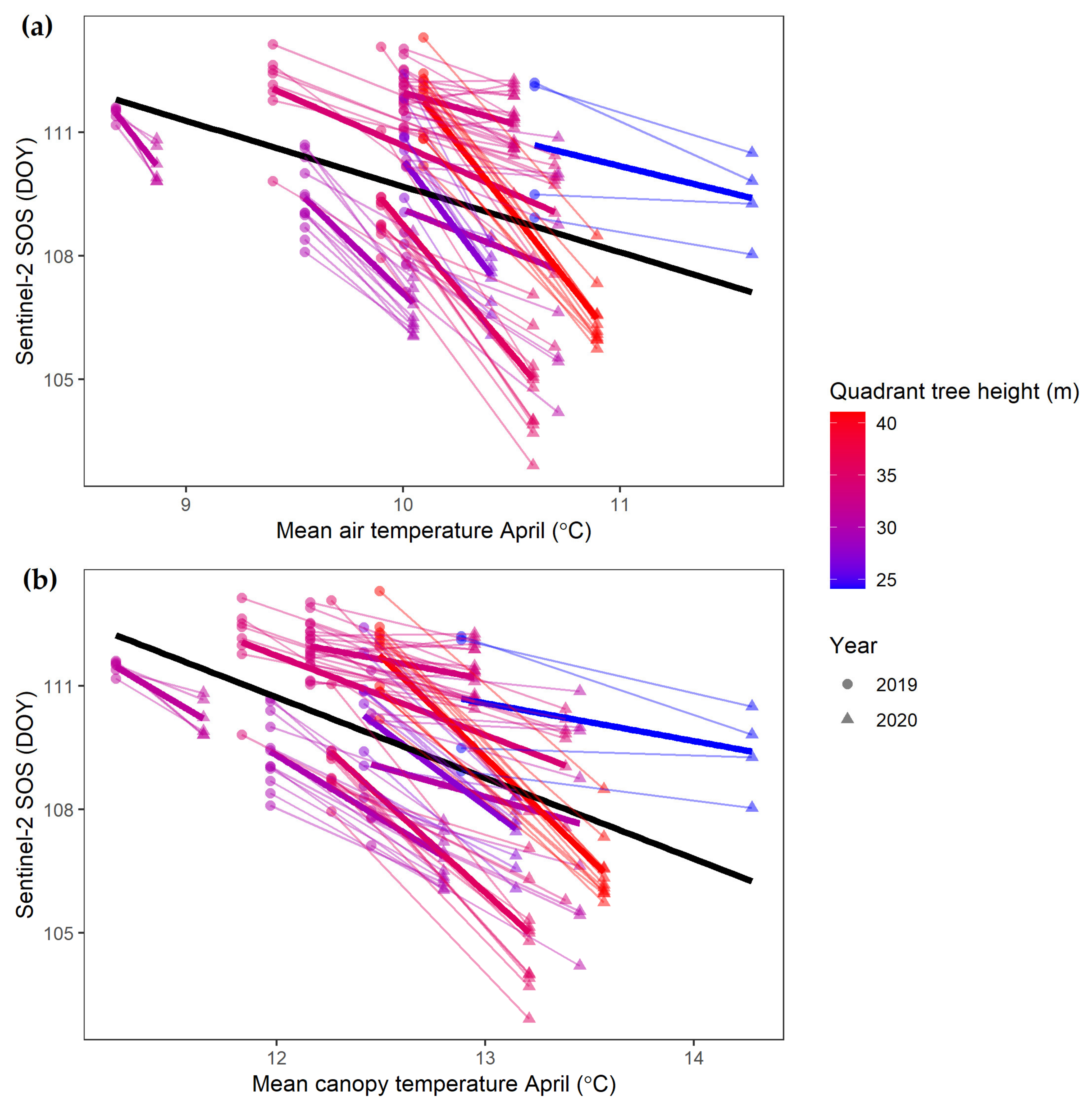
SOS (DOY)	Sentinel-2	CT * height	−2.619 ***	−0.025	−0.082 ***	109.416 ***	184

Note: * p < 0.05; ** p < 0.01; *** p < 0.001.

show that higher canopy temperature advanced F. sylvatica overstory SOS for both camera observations (−2.57 days per °C, p < 0.001) and ground observations (−2.86 days per °C, p < 0.001), using canopy temperature as the only fixed variable in the GLMM. For Sentinel-2 SOS, we found a similar trend of −2.64 days per °C (p < 0.001) when including canopy temperature as the only fixed effect in the model, and −2.62 days per °C (p < 0.001) when additionally including tree height and the interaction between the two fixed effects in the model. In the latter case, we also found a significant interaction between canopy temperature and height, explaining the Sentinel-2 SOS (p < 0.001). In contrast, the canopy temperature did not affect the SOS of the understory for camera observations (−0.18 days per °C, p = 0.57), nor for ground observations (+0.64 days per °C, p = 0.40). A canopy temperature increase of 1 °C led to an increase in vertical mismatch of 2.52 days, as measured by camera observations, and 3.90 days, as measured by ground observations (both p < 0.001).

In Figure 5, we present the significant negative interactions between the climate variables and tree height to explain the Sentinel-2 SOS (Table 2), meaning that the effects of air and canopy temperature were stronger when tree height was higher. In Figure 5, we indeed see that for forests with taller trees (reddish colors), the lines connecting 2019 with 2020 showed a steeper decrease than those lines representing forests with lower trees (bluish colors). This means that for forests with taller trees, effects of air and canopy temperature on Sentinel-2 SOS were stronger than for forests with smaller trees. Note that in Figure 5, we gave all trees within a quadrant the same color for optimal visualization, corresponding to the mean F. sylvatica tree height per quadrant, while we used individual tree height in our GLMMs (Table 2).

Our analysis on all State Forest areas with F. sylvatica as dominant species in the seven quadrants (

Table 3. Pixel mean canopy height effects from separate linear models per quadrant × year predicting Sentinel-2 SOS (Figure 6) and the resulting output for 1 m (understory height) and 30 m (adult tree height). Values under intercept, SOS at 1 m, and SOS at 30 m are in DOY. Height effect is the number of days the SOS is predicted to increase (+) or decrease (−) per m increase in pixel mean canopy height.

	2019				2020
Quadrant	Intercept (DOY)	Height Effect	SOS at 1 m (DOY)	SOS at 30 m (DOY)	Intercept (DOY)	Height Effect	SOS at 1 m (DOY)	SOS at 30 m (DOY)
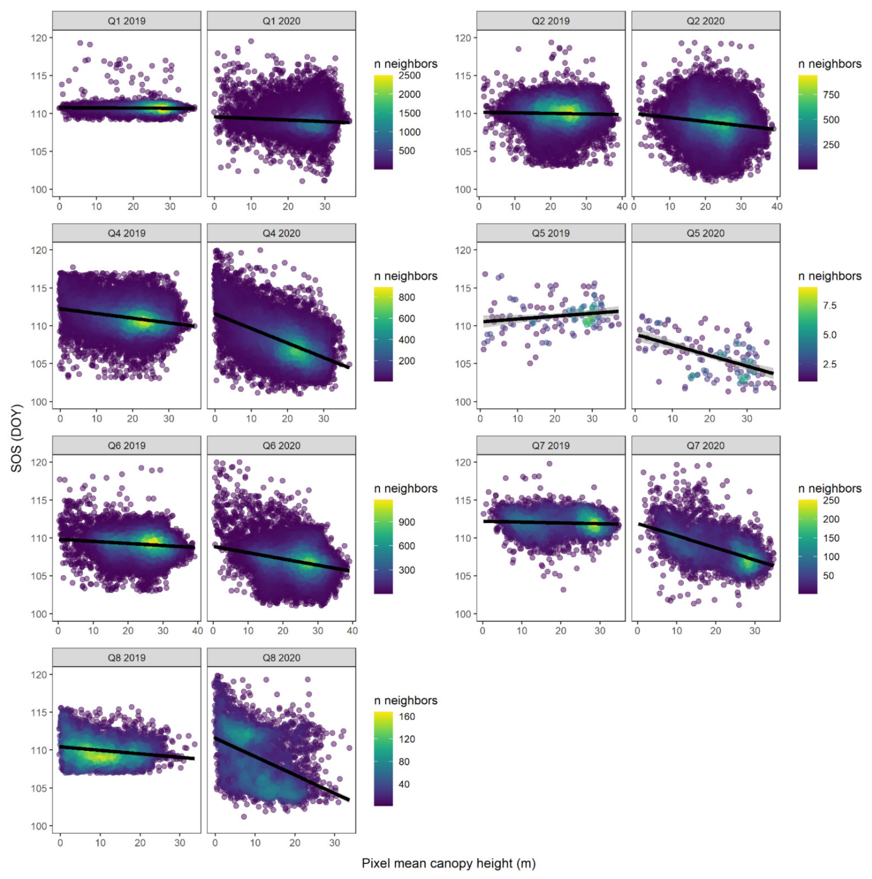
Q1	110.8	−0.003	110.8	110.7	109.6	−0.02	109.6	108.9
Q2	110.2	−0.008	110.2	109.9	110.0	−0.05	110.0	108.4
Q4	112.2	−0.062	112.2	110.4	111.6	−0.19	111.4	105.8
Q5	110.5	+0.038	110.6	111.6	108.9	−0.14	108.7	104.7
Q6	109.9	−0.028	109.8	109.0	109.0	−0.09	108.9	106.4
Q7	112.2	−0.012	112.2	111.9	112.0	−0.16	111.8	107.1
Q8	110.4	−0.046	110.4	109.1	112.0	−0.27	111.8	103.9
Mean	110.9	−0.017	110.9	110.4	110.5	−0.13	110.3	106.5

; Figure 6) revealed that, for all single quadrants and overall, the negative linear relation between Sentinel-2 pixel mean canopy height and Sentinel-2 SOS was stronger in 2020 (mean trend among quadrants of −0.133 days per meter) than in 2019 (mean trend among quadrants of −0.017 days per meter).

This resulted in a relatively similar predicted SOS between years at 1 m (mean DOY of 110.9 in 2019 and mean DOY of 110.3 in 2020), however deviated in predicting the SOS at 30 m (mean DOY of 110.4 in 2019 and mean DOY of 106.5 in 2020) (Table 3; Figure 6).

4. Discussion

4.1. Over- and Understory Phenology Response to Climatic Drivers

For both camera and ground observations, F. sylvatica overstory advanced more than F. sylvatica understory in 2020, with the warmer and higher radiant April, compared to 2019, with a cooler and lower radiant April. Furthermore, overstory SOS was directly related to vertical mismatch with a ratio of roughly 1:1.

Matching these results, both our camera and ground observations revealed that F. sylvatica overstory and understory phenology responded differently to climatic drivers: the overstory advanced more with higher canopy temperature, a variable integrating radiation and air temperature, than the understory did.

The significant advances of overstory SOS with higher canopy temperature were very close to each other for the three different methods: −2.86 days per °C for ground observations, −2.57 days per °C for camera observations, and −2.62 days per °C for Sentinel-2 observations. These rates closely matched the mean advance of 2.5 days per °C temperature increase reported by Menzel et al. [1] for all recorded species together.

However, for the understory, we did not observe phenological advancing with higher canopy temperatures, indicating again that phenology of F. sylvatica foliage in the understory may be less responsive to climate change than phenology of F. sylvatica foliage in the overstory.

4.2. Vertical Mismatch

As a result, for both camera and ground observations, a higher canopy temperature led to a decreased phenological escape of the understory, meaning an increased vertical mismatch within F. sylvatica. We found a higher increase in vertical mismatch with canopy temperature for ground observations than for camera observations. That might be related to the fact that for the ground observations of the understory, juveniles were exclusively selected, while the camera understory ROIs also covered lower parts of taller trees. Furthermore, foliage further away from the camera might have also slightly exceeded the lowest two meters of the forest. This reasoning is plausible since the closer to the forest floor, the higher the temperature and radiation buffering [28].

Our results indicate an understory being relatively irresponsive to climate variables, unlike the highly susceptive overstory. This may cause shifting matches between overstory and understory phenology in the future, as not only the widely reported worldwide temperatures are continuing to rise, but increasing trends for global radiation were likewise reported. In Bavaria, between 1951 and 2020, sunshine duration increased yearly by 7.7%, by 10.7% in spring (mean of March, April, and May), and, in April specifically, by 23.8%. Zooming out to Germany, the respective numbers were quite similar (8.7%, 11.9%, and 23.2%) [83]. Moreover, for the entirety of Europe, covering the whole area in which F. sylvatica naturally occurs, Pfeifroth et al. [84] reported an overall brightening since the 1980s, with a rate of between 1.9 and 2.4 W/m²/decade. If climate change, in terms of air warming and increasing radiation, will keep advancing overstory SOS, our results suggest that the vertical mismatch between forest layers may increase for F. sylvatica. Or, in the words of Jacques et al. [30], the understory will be less able to “phenologically escape”. We can explain these results by the buffering capacity of forest overstory to climate variables, making them fluctuate less in the understory [10]. More specifically, results from Hertel et al. [24] indicated that the difference in PAR between the overstory and understory was more pronounced with clear-sky conditions than with overcast-sky conditions. Furthermore, in April, the month in which the SOS occurred in all cases, the angle of the sun relative to the horizon was still relatively low in our study area, which additionally negatively affected the amount of PAR that was able to penetrate a canopy, but only on clear-sky days [85]. To prove these hypotheses of microclimatic differences between the overstory and understory, we recommend conducting future studies to measure both the understory and overstory temperature and radiation at each study site.

Our results were in line with the results from Heberling et al. [9], who found a lower response rate to increased weather station-derived temperature for flower phenology of the herbaceous understory layer compared to canopy phenology of the overstory. Our finding, that the same principle applies intra-specifically to F. sylvatica foliage, is new and implies important ecological effects, as well as methodological consequences, for the field of remote sensing.

4.3. Ecological Consequences and Forest Management

Ecologically and on the population level of F. sylvatica, increased vertical mismatch between the overstory and understory of the same species will drastically decrease the amount of light that reaches the understory in the favorable time period that it uses to phenologically escape [30]. In this way, photosynthesis, carbon uptake, and the growth of the understory may be decreased [23] and the establishment of regeneration might be hampered. As understory is the overstory of the future, this might highly affect the future of deciduous forests [18], at least those in which F. sylvatica is the dominating species, which, in turn, might affect wood production and animal habitats. We suggest future research to test if these patterns can be generalized to other main deciduous tree species in temperate forests.

Nevertheless, the lower phenological response rate of the understory to temperature might decrease its susceptibility to late-frost events after leafout, and, in that way, the mechanism also acts as a buffer. However, Jones et al. [26] and Seiwa [27] showed that, for Acer rubrum and Acer mono seedlings, this late-frost risk was negligible compared to the huge advantage of leafing out before the overstory.

On the other hand, phenological mismatches with higher trophic levels, enhanced by climate change, might be buffered by a more stable understory that is less susceptive to change. This will especially count for herbivores, which are exclusively dependent on the understory [37], such as roe deer, and also for animals, which are theoretically able to move among forest layers to track vertical variability in leaf and flower phenology. However, in reality, most arthropods are highly stratified to a single forest layer for foraging [17]. If this is the understory, our findings indicate that they will be affected differently than in case of the overstory.

Our results, and these potential ecological consequences, should be accounted for in decision making in forest management. Silvicultural measures in regeneration stands, such as selective cutting intended to create gaps in the overstory, are often designed to regulate the radiation gain in the understory in such a way that the regeneration is promoted in its growth. If the phenological escape became smaller due to climate change, including higher temperatures and global radiation, then the (natural) regeneration would have poorer chances of growing up underneath older stands. This negative effect would then have to be avoided by more intense selective cuttings of trees with crowns in the upper layer. This, in turn, could reduce the ecological services of forests, such as climate (temperature) mitigation, which are more pronounced in closed stands.

4.4. Methodological Consequences

Our results showed that erroneous ecological conclusions might be drawn when generalizing climate effects on forest phenology to only two dimensions, which is generally done using Sentinel-2 or other multispectral remote sensing data.

The canopy temperature response rate of the Sentinel-2 derived SOS was closer to those of the ground and camera derived overstory SOS than to those of the understory SOS. This means that Sentinel-2 data tended to overestimate climate effects on phenology of the forest as a whole. Among all studies in which overstory and understory phenology are disentangled and compared with satellite data, we are reporting this pattern for the first time. In contrast, Ahl et al. [35] and Ryu et al. [38] found MODIS-derived phenology to be better matching with understory phenological ground observations than with overstory phenological ground observations. However, those studies reported consistently earlier spring starts for the understory than for the overstory, just as Augspurger and Barlett [19], Richardson and O’Keefe [20], and Liu et al. [49] did. In those cases, as the understory became visible first, it is logical that this layer was prevailing in the remotely sensed phenology signal. In contrast to those publications, in our study, the phenology of the understory mostly lagged behind that of the overstory (for more than half of the study sites the vertical mismatch was >0). In those cases, obviously, it was mainly the overstory that could be sensed from above. We can also explain the deviation from the earlier studies with specific weather conditions in our study years. April 2020 was the April with the highest sunshine duration (with an anomaly of +93.1% compared to 1961–1990), and the months March, April, and May, taken together, formed the spring with the highest sunshine duration (with an anomaly of +49.1% compared to 1961–1990) since the start of observations in Bavaria in 1951. Furthermore, April 2019 was, with an anomaly of +40.8% in sunshine duration compared to 1961–1990, also relatively sunshine-rich. Additionally, mean April temperatures in Bavaria were also relatively high in both years: 10.3 °C in 2020 (+3.3 °C compared to 1961–1990) and 9.4 °C in 2019 (+2.4 °C compared to 1961–1990) [83,86]. Consequently, springs in the study years were likely warmer and had higher radiation levels than the aforementioned studies, increasing the likelihood of higher vertical mismatch and, in turn, the likelihood that the overstory was visible earlier than the understory in the satellite signal.

In line with these results, the significant interaction between tree height and canopy temperature explaining the Sentinel-2 SOS indicates that the higher the forest trees, the stronger the effect of temperature and radiation, and the larger the phenological difference between the two years. We argue that this is the case because the relative proportion of the understory, which was responding less to canopy temperature, was lower in the vertically integrated Sentinel-2 signal when the average tree height was higher for two reasons: first, there was relatively more biomass, such as branches, of the overstory trees present in pixels with a taller tree canopy, blocking the view on the understory, and second, when fully stocked, there was less understory present underneath taller trees because of the lower light conditions in the growing season. Several studies used the same reasoning to explain higher understory appearance in sparser coniferous forests [36,87,88].

Our larger scale analysis on all beech forest stands revealed patterns within each quadrant confirming this height-climate interaction: comparing the SOS responses to pixel mean canopy height between the two years, we systematically observed rates with higher decreasing magnitudes in 2020, which had a warmer and higher radiant April, compared to 2019, which had a cooler and less radiant April. We can explain the relatively low SOS response rates to pixel mean canopy height in 2019 by our result that, on average, the understory greened up before the overstory that year. Intuitively, in such cases, we would have expected an increasing response of SOS to height, which only Q5 demonstrated (+0.038 days per degree warming, p < 0.001). We explain a more or less equal SOS for different pixel mean canopy heights however by the fact that pixels with both low as well as high canopies contained understory. In the warmer and more radiant spring of 2020, we observed, for all seven quadrants, a steeper decreasing SOS with increasing pixel mean canopy height. As higher pixels will again have relatively higher proportions of overstory compared to lower pixels, this result is in line with an earlier greening overstory than understory in 2020.

4.5. Future Research Directions

The study of phenology by remote sensing is, in the literature, generally defined as land surface phenology (LSP) [89]. However, we argue that “land” per definition is not a “surface”, but rather a three-dimensional space. This pre-eminently applies to forests, as they are a green land use type with a relatively large vertical component upon which many ecological processes depend. This study proved that generalizing its phenology to only two-dimensions might lead to oversimplified conclusions on climate effects. In warm, high radiant springs, the overall forest phenological advance to warming might be overestimated because there is an invisible understory layer below which responds later. On the contrary, in colder, less radiant springs, when the understory SOS takes place before the overstory SOS, the sensed phenological advance by warming depends on the canopy height and density: for higher or denser forests the phenological advance might be relatively overestimated because of a higher proportion of overstory in the signal, while in lower or sparser forests it might be underestimated because of a higher proportion of understory in the signal.

Methodologically, we recommend that, when using Sentinel-2 or any other spectral satellite remote sensing product in future phenological studies in temperate deciduous forests, ground and camera observations should be conducted as well to disentangle overstory from understory. The application of UAVs [46], or satellite sensors with a higher spatial resolution such as PlanetScope data (3 m resolution) [90], is also promising for this purpose, as pixels showing pure understory might be visible through smaller gaps in the canopy. Furthermore, for the case of UAVs, height can photogrammetrically be derived on such a fine scale using the overlap of images. An important requirement thereby is that the temporal resolution should be high enough to cover periods with phenological change. Furthermore, we recommend investigating the use of indices other than NDVI, such as the two-band enhanced vegetation index (EVI2) or the plant phenology index (PPI), as these may saturate less quickly at higher biomass levels and, therefore, might perform better in predicting vegetation phenology [91] and potential vertical mismatch. Furthermore, especially when moving away from temperate deciduous forests, it is important to carefully choose the method to derive the SOS, as White et al. [43] found that the ordinal rank of SOS methods differs among ecoregions. Among others, the smoothing method of raw data should be carefully considered, as, in some cases or specific ecoregions, methods other than double-logistic curve-fitting, such as HANTS or SG, might be more appropriate, e.g., [43,92]. Moreover, recent studies, e.g., [93], showed that machine learning techniques might be promising as they are outperforming other methods to derive SOS, validated by ground observations.

Ecologically, since Vitasse et al. [21] proved that phenological escaping of the understory is determined ontogenetically, and since our findings suggest increased phenological mismatch with warmer and higher radiant springs, we expect that climate change proceeds faster than species are able to ontogenetically adapt. An adaptation strategy would be that the ontogenetic phenological differences also increase, by which the understory will stay relatively able to keep phenologically escaping. More research and, most importantly, more study years are needed to investigate this kind of (micro)evolution in response to further climate change.

As Teuling et al. [94] found in observational evidence for higher cloud cover over large forest regions in Western Europe, it may be that in regions with large proportions of forest cover, radiation and temperature changes are mitigated, thereby suggesting that the vertical mismatch found in this study may be less pronounced. Therefore, our findings are not only relevant to consider for small scale forest management, but also for large scale land use decisions. We support further research on the interaction between land use and climate change.

5. Conclusions

Cameras and ground observations revealed that increased April canopy temperature, integrating air temperature, and site-specific radiation, advanced the overstory phenology, but not the understory phenology, leading to a decrease of the classical phenological escape of the understory relative to the overstory and, therefore, to an increase in vertical mismatch. Furthermore, higher trees and forest canopies had a higher sensitivity to temperature than lower trees and forests, as we found through the Sentinel-2 data.

These findings may have major ecological and economical effects, as well as methodological consequences, for remote sensing studies. Ecologically and economically, they indicate that—for this specific pathway—climate change may render (natural) regeneration under older stands more difficult, but decrease potential damage by spring late-frost events and buffer phenological mismatches with higher trophic levels. Methodologically, the warmer and more radiant a spring, the more likely it is that we sense the overstory without the understory in the signal from Sentinel-2. Due to this climate dependency, remotely sensed signals from above, which generalize forests to a 2D-surface, such as those from Sentinel-2, might be misinterpreted. This may lead to incorrect conclusions about the relationship between climate change and forest phenology, and on how able these forests are to mitigate these effects. We recommend our findings be taken into account in future forest management and land use decisions, as well as in further research on remote sensing of forest phenology.

References

- Menzel, A.; Sparks, T.H.; Estrella, N.; Koch, E.; Aasa, A.; Ahas, R.; Alm-Kübler, K.; Bissolli, P.; Braslavská, O.G.; Briede, A. European phenological response to climate change matches the warming pattern. Glob. Chang. Biol. 2006, 12, 1969–1976. [Google Scholar] [CrossRef]
- Cannell, M.; Smith, R. Climatic warming, spring budburst and forest damage on trees. J. Appl. Ecol. 1986, 23, 177–191. [Google Scholar] [CrossRef]
- Gu, L.; Hanson, P.J.; Post, W.M.; Kaiser, D.P.; Yang, B.; Nemani, R.; Pallardy, S.G.; Meyers, T. The 2007 eastern US spring freeze: Increased cold damage in a warming world? BioScience 2008, 58, 253–262. [Google Scholar] [CrossRef]
- Plard, F.; Gaillard, J.-M.; Coulson, T.; Hewison, A.J.M.; Delorme, D.; Warnant, C.; Bonenfant, C. Mismatch Between Birth Date and Vegetation Phenology Slows the Demography of Roe Deer. PLoS Biol. 2014, 12, e1001828. [Google Scholar] [CrossRef] [PubMed]
- Renner, S.S.; Zohner, C.M. Climate Change and Phenological Mismatch in Trophic Interactions Among Plants, Insects, and Vertebrates. Annu. Rev. Ecol. Evol. Syst. 2018, 49, 165–182. [Google Scholar] [CrossRef]
- Thackeray, S.J.; Sparks, T.H.; Frederiksen, M.; Burthe, S.; Bacon, P.J.; Bell, J.R.; Botham, M.S.; Brereton, T.M.; Bright, P.W.; Carvalho, L. Trophic level asynchrony in rates of phenological change for marine, freshwater and terrestrial environments. Glob. Chang. Biol. 2010, 16, 3304–3313. [Google Scholar] [CrossRef] [Green Version]
- Visser, M.E.; Van Noordwijk, A.J.; Tinbergen, J.M.; Lessells, C.M. Warmer springs lead to mistimed reproduction in great tits (Parus major). Proc. R. Soc. B Boil. Sci. 1998, 265, 1867–1870. [Google Scholar] [CrossRef] [Green Version]
- Voigt, W.; Perner, J.; Davis, A.J.; Eggers, T.; Schumacher, J.; Bährmann, R.; Fabian, B.; Heinrich, W.; Köhler, G.; Lichter, D. Trophic levels are differentially sensitive to climate. Ecology 2003, 84, 2444–2453. [Google Scholar] [CrossRef] [Green Version]
- Heberling, J.M.; McDonough MacKenzie, C.; Fridley, J.D.; Kalisz, S.; Primack, R.B. Phenological mismatch with trees reduces wildflower carbon budgets. Ecol. Lett. 2019, 22, 616–623. [Google Scholar] [CrossRef]
- Landuyt, D.; De Lombaerde, E.; Perring, M.P.; Hertzog, L.R.; Ampoorter, E.; Maes, S.L.; De Frenne, P.; Ma, S.; Proesmans, W.; Blondeel, H. The functional role of temperate forest understorey vegetation in a changing world. Glob. Chang. Biol. 2019, 25, 3625–3641. [Google Scholar] [CrossRef]
- Post, E.; Pedersen, C.; Wilmers, C.C.; Forchhammer, M.C. Warming, plant phenology and the spatial dimension of trophic mismatch for large herbivores. Proc. R. Soc. B Boil. Sci. 2008, 275, 2005–2013. [Google Scholar] [CrossRef] [PubMed] [Green Version]
- Wang, C.; Tang, Y.; Chen, J. Plant phenological synchrony increases under rapid within-spring warming. Sci. Rep. 2016, 6, 1–7. [Google Scholar] [CrossRef] [Green Version]
- Zohner, C.M.; Mo, L.; Renner, S.S. Global warming reduces leaf-out and flowering synchrony among individuals. eLife 2018, 7, e40214. [Google Scholar] [CrossRef]
- Chen, L.; Huang, J.-G.; Ma, Q.; Hänninen, H.; Rossi, S.; Piao, S.; Bergeron, Y. Spring phenology at different altitudes is becoming more uniform under global warming in Europe. Glob. Chang. Biol. 2018, 24, 3969–3975. [Google Scholar] [CrossRef]
- Vitasse, Y.; Signarbieux, C.; Fu, Y.H. Global warming leads to more uniform spring phenology across elevations. Proc. Natl. Acad. Sci. USA 2018, 115, 1004–1008. [Google Scholar] [CrossRef] [PubMed] [Green Version]
- Donnelly, A.; Yu, R. Temperate deciduous shrub phenology: The overlooked forest layer. Int. J. Biometeorol. 2019, 65, 1–13. [Google Scholar] [CrossRef]
- Ulyshen, M.D. Arthropod vertical stratification in temperate deciduous forests: Implications for conservation-oriented management. For. Ecol. Manag. 2011, 261, 1479–1489. [Google Scholar] [CrossRef]
- Kwit, M.C.; Rigg, L.S.; Goldblum, D. Sugar maple seedling carbon assimilation at the northern limit of its range: The importance of seasonal light. Can. J. For. Res. 2010, 40, 385–393. [Google Scholar] [CrossRef]
- Augspurger, C.K.; Bartlett, E.A. Differences in leaf phenology between juvenile and adult trees in a temperate deciduous forest. Tree Physiol. 2003, 23, 517–525. [Google Scholar] [CrossRef] [PubMed]
- Richardson, A.D.; O’Keefe, J. Phenological differences between understory and overstory. In Phenology of Ecosystem Processes; Springer: New York, NY, USA, 2009; pp. 87–117. [Google Scholar]
- Vitasse, Y. Ontogenic changes rather than difference in temperature cause understory trees to leaf out earlier. New Phytol. 2013, 198, 149–155. [Google Scholar] [CrossRef] [PubMed]
- Fu, Y.H.; Piao, S.; Op de Beeck, M.; Cong, N.; Zhao, H.; Zhang, Y.; Menzel, A.; Janssens, I.A. Recent spring phenology shifts in western C entral E urope based on multiscale observations. Glob. Ecol. Biogeogr. 2014, 23, 1255–1263. [Google Scholar] [CrossRef]
- Gill, D.S.; Amthor, J.S.; Bormann, F.H. Leaf phenology, photosynthesis, and the persistence of saplings and shrubs in a mature northern hardwood forest. Tree Physiol. 1998, 18, 281–289. [Google Scholar] [CrossRef]
- Hertel, C.; Leuchner, M.; Menzel, A. Vertical variability of spectral ratios in a mature mixed forest stand. Agric. For. Meteorol. 2011, 151, 1096–1105. [Google Scholar] [CrossRef]
- Jolly, W.M.; Nemani, R.; Running, S.W. Enhancement of understory productivity by asynchronous phenology with overstory competitors in a temperate deciduous forest. Tree Physiol. 2004, 24, 1069–1071. [Google Scholar] [CrossRef] [Green Version]
- Jones, R.H.; Allen, B.P.; Sharitz, R.R. Why do early-emerging tree seedlings have survival advantages?: A test using Acer rubrum (Aceraceae). Am. J. Bot. 1997, 84, 1714–1718. [Google Scholar] [CrossRef]
- Seiwa, K. Advantages of early germination for growth and survival of seedlings of Acer mono under different overstorey phenologies in deciduous broad-leaved forests. J. Ecol. 1998, 86, 219–228. [Google Scholar] [CrossRef]
- De Frenne, P.; Zellweger, F.; Rodriguez-Sanchez, F.; Scheffers, B.R.; Hylander, K.; Luoto, M.; Vellend, M.; Verheyen, K.; Lenoir, J. Global buffering of temperatures under forest canopies. Nat. Ecol. Evol. 2019, 3, 744–749. [Google Scholar] [CrossRef]
- Bolte, A.; Czajkowski, T.; Cocozza, C.; Tognetti, R.; De Miguel, M.; Pšidová, E.; Ditmarová, Ĺ.; Dinca, L.; Delzon, S.; Cochard, H. Desiccation and mortality dynamics in seedlings of different European beech (Fagus sylvatica L.) populations under extreme drought conditions. Front. Plant Sci. 2016, 7, 751. [Google Scholar] [CrossRef] [Green Version]
- Jacques, M.H.; Lapointe, L.; Rice, K.; Montgomery, R.A.; Stefanski, A.; Reich, P.B. Responses of two understory herbs, Maianthemum canadense and Eurybia macrophylla, to experimental forest warming: Early emergence is the key to enhanced reproductive output. Am. J. Bot. 2015, 102, 1610–1624. [Google Scholar] [CrossRef] [PubMed] [Green Version]
- Vitasse, Y.; Baumgarten, F.; Zohner, C.M.; Kaewthongrach, R.; Fu, Y.H.; Walde, M.G.; Moser, B. Impact of microclimatic conditions and resource availability on spring and autumn phenology of temperate tree seedlings. New Phytol. 2021, 232, 537–550. [Google Scholar] [CrossRef]
- Bennie, J.; Huntley, B.; Wiltshire, A.; Hill, M.O.; Baxter, R. Slope, aspect and climate: Spatially explicit and implicit models of topographic microclimate in chalk grassland. Ecol. Model. 2008, 216, 47–59. [Google Scholar] [CrossRef]
- Myneni, R.B.; Keeling, C.; Tucker, C.J.; Asrar, G.; Nemani, R.R. Increased plant growth in the northern high latitudes from 1981 to 1991. Nature 1997, 386, 698–702. [Google Scholar] [CrossRef]
- White, M.A.; Thornton, P.E.; Running, S.W. A continental phenology model for monitoring vegetation responses to interannual climatic variability. Glob. Biogeochem. Cycles 1997, 11, 217–234. [Google Scholar] [CrossRef]
- Ahl, D.E.; Gower, S.T.; Burrows, S.N.; Shabanov, N.V.; Myneni, R.B.; Knyazikhin, Y. Monitoring spring canopy phenology of a deciduous broadleaf forest using MODIS. Remote Sens. Environ. 2006, 104, 88–95. [Google Scholar] [CrossRef] [Green Version]
- Eriksson, H.M.; Eklundh, L.; Kuusk, A.; Nilson, T. Impact of understory vegetation on forest canopy reflectance and remotely sensed LAI estimates. Remote Sens. Environ. 2006, 103, 408–418. [Google Scholar] [CrossRef]
- Tuanmu, M.-N.; Viña, A.; Bearer, S.; Xu, W.; Ouyang, Z.; Zhang, H.; Liu, J. Mapping understory vegetation using phenological characteristics derived from remotely sensed data. Remote Sens. Environ. 2010, 114, 1833–1844. [Google Scholar] [CrossRef]
- Ryu, Y.; Lee, G.; Jeon, S.; Song, Y.; Kimm, H. Monitoring multi-layer canopy spring phenology of temperate deciduous and evergreen forests using low-cost spectral sensors. Remote Sens. Environ. 2014, 149, 227–238. [Google Scholar] [CrossRef]
- Rankine, C.; Sánchez-Azofeifa, G.; Guzmán, J.A.; Espirito-Santo, M.; Sharp, I. Comparing MODIS and near-surface vegetation indexes for monitoring tropical dry forest phenology along a successional gradient using optical phenology towers. Environ. Res. Lett. 2017, 12, 105007. [Google Scholar] [CrossRef] [Green Version]
- Pisek, J.; Chen, J.M.; Kobayashi, H.; Rautiainen, M.; Schaepman, M.E.; Karnieli, A.; Sprinstin, M.; Ryu, Y.; Nikopensius, M.; Raabe, K. Retrieval of seasonal dynamics of forest understory reflectance from semiarid to boreal forests using MODIS BRDF data. J. Geophys. Res. Biogeosci. 2016, 121, 855–863. [Google Scholar] [CrossRef] [Green Version]
- Misra, G.; Buras, A.; Heurich, M.; Asam, S.; Menzel, A. LiDAR derived topography and forest stand characteristics largely explain the spatial variability observed in MODIS land surface phenology. Remote Sens. Environ. 2018, 218, 231–244. [Google Scholar] [CrossRef]
- Rodriguez-Galiano, V.; Dash, J.; Atkinson, P.M. Intercomparison of satellite sensor land surface phenology and ground phenology in Europe. Geophys. Res. Lett. 2015, 42, 2253–2260. [Google Scholar] [CrossRef] [Green Version]
- White, M.A.; de Beurs, K.M.; Didan, K.; Inouye, D.W.; Richardson, A.D.; Jensen, O.P.; O’Keefe, J.; Zhang, G.; Nemani, R.R.; van Leeuwen, W.J. Intercomparison, interpretation, and assessment of spring phenology in North America estimated from remote sensing for 1982–2006. Glob. Chang. Biol. 2009, 15, 2335–2359. [Google Scholar] [CrossRef]
- Keenan, T.; Darby, B.; Felts, E.; Sonnentag, O.; Friedl, M.; Hufkens, K.; O’Keefe, J.; Klosterman, S.; Munger, J.W.; Toomey, M. Tracking forest phenology and seasonal physiology using digital repeat photography: A critical assessment. Ecol. Appl. 2014, 24, 1478–1489. [Google Scholar] [CrossRef] [PubMed] [Green Version]
- Klosterman, S.; Richardson, A.D. Observing spring and fall phenology in a deciduous forest with aerial drone imagery. Sensors 2017, 17, 2852. [Google Scholar] [CrossRef] [PubMed] [Green Version]
- Klosterman, S.; Melaas, E.; Wang, J.; Martinez, A.; Frederick, S.; O’Keefe, J.; Orwig, D.A.; Wang, Z.; Sun, Q.; Schaaf, C. Fine-scale perspectives on landscape phenology from unmanned aerial vehicle (UAV) photography. Agric. For. Meteorol. 2018, 248, 397–407. [Google Scholar] [CrossRef]
- Vrieling, A.; Meroni, M.; Darvishzadeh, R.; Skidmore, A.K.; Wang, T.; Zurita-Milla, R.; Oosterbeek, K.; O’Connor, B.; Paganini, M. Vegetation phenology from Sentinel-2 and field cameras for a Dutch barrier island. Remote Sens. Environ. 2018, 215, 517–529. [Google Scholar] [CrossRef]
- Hufkens, K.; Friedl, M.; Sonnentag, O.; Braswell, B.H.; Milliman, T.; Richardson, A.D. Linking near-surface and satellite remote sensing measurements of deciduous broadleaf forest phenology. Remote Sens. Environ. 2012, 117, 307–321. [Google Scholar] [CrossRef]
- Liu, N.; Garcia, M.; Singh, A.; Clare, J.D.; Stenglein, J.L.; Zuckerberg, B.; Kruger, E.L.; Townsend, P.A. Trail camera networks provide insights into satellite-derived phenology for ecological studies. Int. J. Appl. Earth Obs. Geoinf. 2021, 97, 102291. [Google Scholar] [CrossRef]
- Redlich, S.; Zhang, J.; Benjamin, C.; Dhillon, M.S.; Englmeier, J.; Ewald, J.; Fricke, U.; Ganuza, C.; Haensel, M.; Hovestadt, T. Disentangling effects of climate and land use on biodiversity and ecosystem services-a multi-scale experimental design. bioRxiv 2021. [Google Scholar] [CrossRef]
- Gressler, E.; Jochner, S.; Capdevielle-Vargas, R.M.; Morellato, L.P.C.; Menzel, A. Vertical variation in autumn leaf phenology of Fagus sylvatica L. in southern Germany. Agric. For. Meteorol. 2015, 201, 176–186. [Google Scholar] [CrossRef]
- Ammer, C. Impact of ungulates on structure and dynamics of natural regeneration of mixed mountain forests in the Bavarian Alps. For. Ecol. Manag. 1996, 88, 43–53. [Google Scholar] [CrossRef]
- Motta, R. Impact of wild ungulates on forest regeneration and tree composition of mountain forests in the Western Italian Alps. For. Ecol. Manag. 1996, 88, 93–98. [Google Scholar] [CrossRef]
- Putman, R.; Moore, N. Impact of deer in lowland Britain on agriculture, forestry and conservation habitats. Mammal Rev. 1998, 28, 141–164. [Google Scholar] [CrossRef]
- Sonnentag, O.; Hufkens, K.; Teshera-Sterne, C.; Young, A.M.; Friedl, M.; Braswell, B.H.; Milliman, T.; O’Keefe, J.; Richardson, A.D. Digital repeat photography for phenological research in forest ecosystems. Agric. For. Meteorol. 2012, 152, 159–177. [Google Scholar] [CrossRef]
- Richardson, A.D.; Hufkens, K.; Milliman, T.; Aubrecht, D.M.; Chen, M.; Gray, J.M.; Johnston, M.R.; Keenan, T.F.; Klosterman, S.T.; Kosmala, M. Tracking vegetation phenology across diverse North American biomes using PhenoCam imagery. Sci. Data 2018, 5, 1–24. [Google Scholar] [CrossRef]
- Beck, P.S.; Atzberger, C.; Høgda, K.A.; Johansen, B.; Skidmore, A.K. Improved monitoring of vegetation dynamics at very high latitudes: A new method using MODIS NDVI. Remote Sens. Environ. 2006, 100, 321–334. [Google Scholar] [CrossRef]
- Filippa, G.; Cremonese, E.; Migliavacca, M.; Galvagno, M.; Forkel, M.; Wingate, L.; Tomelleri, E.; Di Cella, U.M.; Richardson, A.D. Phenopix: AR package for image-based vegetation phenology. Agric. For. Meteorol. 2016, 220, 141–150. [Google Scholar] [CrossRef] [Green Version]
- R Core Team. R: A Language and Environment for Statistical Computing; R Foundation for Statistical Computing: Vienna, Austria, 2020. [Google Scholar]
- Oliver, C.D.; Larson, B.C. Forest Stand Dynamics: Updated Edition; John Wiley and Sons: Hoboken, NJ, USA, 1996. [Google Scholar]
- Meier, U. (Ed.) BBCH-Monograph: Growth Stages of Mono-and Dicotyledonous Plants, 2nd ed.; Technical Report; Federal Biological Research Centre for Agriculture and Forestry: Bonn, Germany, 2001. [Google Scholar]
- Lange, M.; Doktor, D. Phenex: Auxiliary Functions for Phenological Data Analysis, R Package Version 1.4-5. 2017. Available online: https://rdrr.io/cran/phenex/ (accessed on 4 October 2021).
- Fischer, A. A model for the seasonal variations of vegetation indices in coarse resolution data and its inversion to extract crop parameters. Remote Sens. Environ. 1994, 48, 220–230. [Google Scholar] [CrossRef]
- White, K.; Pontius, J.; Schaberg, P. Remote sensing of spring phenology in northeastern forests: A comparison of methods, field metrics and sources of uncertainty. Remote Sens. Environ. 2014, 148, 97–107. [Google Scholar] [CrossRef]
- Ranghetti, L.; Boschetti, M.; Nutini, F.; Busetto, L. “sen2r”: An R toolbox for automatically downloading and preprocessing Sentinel-2 satellite data. Comput. Geosci. 2020, 139, 104473. [Google Scholar] [CrossRef]
- Malingreau, J. The vegetation index and the study of vegetation dynamics. In Applications of Remote Sensing to Agrometeorology; Springer: New York, NY, USA, 1989; pp. 285–303. [Google Scholar]
- Riedel, T.; Hennig, P.; Kroiher, F.; Polley, H.; Schmitz, F.; Schwitzgebel, F. Die dritte Bundeswaldinventur (BWI 2012). In Inventur-und Auswertemethoden; Johann Heinrich von Thünen Institute: Braunschweig, Germany, 2017. [Google Scholar]
- Zhang, X.; Wang, J.; Gao, F.; Liu, Y.; Schaaf, C.; Friedl, M.; Yu, Y.; Jayavelu, S.; Gray, J.; Liu, L. Exploration of scaling effects on coarse resolution land surface phenology. Remote Sens. Environ. 2017, 190, 318–330. [Google Scholar] [CrossRef] [Green Version]
- Misra, G.; Buras, A.; Menzel, A. Effects of different methods on the comparison between land surface and ground phenology—A methodological case study from south-western Germany. Remote Sens. 2016, 8, 753. [Google Scholar] [CrossRef] [Green Version]
- Roussel, J.-R.; Auty, D.; Coops, N.C.; Tompalski, P.; Goodbody, T.R.; Meador, A.S.; Bourdon, J.-F.; de Boissieu, F.; Achim, A. lidR: An R package for analysis of Airborne Laser Scanning (ALS) data. Remote Sens. Environ. 2020, 251, 112061. [Google Scholar] [CrossRef]
- DWD Climate Data Center (CDC). Annual Grids of Monthly Averaged Daily Air Temperature (2 m) Over Germany; Version v1.0; DWD: Offenbach am Main, Germany, 2020. [Google Scholar]
- Fu, P.; Rich, P.M. Design and implementation of the Solar Analyst: An ArcView extension for modeling solar radiation at landscape scales. In Proceedings of the 9th Annual ESRI User Conference, San Diego, CA, USA, 26–30 July 1999; pp. 1–31. [Google Scholar]
- Allen, R.G.; Trezza, R.; Tasumi, M. Analytical integrated functions for daily solar radiation on slopes. Agric. For. Meteorol. 2006, 139, 55–73. [Google Scholar] [CrossRef]
- Huang, S.; Rich, P.M.; Crabtree, R.L.; Potter, C.S.; Fu, P. Modeling monthly near-surface air temperature from solar radiation and lapse rate: Application over complex terrain in Yellowstone National Park. Phys. Geogr. 2008, 29, 158–178. [Google Scholar] [CrossRef]
- Ashcroft, M.B. A method for improving landscape scale temperature predictions and the implications for vegetation modelling. Ecol. Model. 2006, 197, 394–404. [Google Scholar] [CrossRef] [Green Version]
- Bates, D.; Maechler, M.; Bolker, B.; Walker, S. Ime4: Linear Mixed-Effects Models Using Eigen and S4. R package Version 1.1-27.1. 2021. Available online: https://cran.r-project.org/web/packages/lme4/ (accessed on 4 October 2021).
- Hijmans, R.J.; Van Etten, J. raster: Geographic Data Analysis and Modeling. R Package Version 2.5–8. 2016. Available online: https://cran.r-project.org/web/packages/raster/ (accessed on 4 October 2021).
- Leutner, B.; Horning, N.; Schwalb-Willmann, J.R. Tools for Remote Sensing Data Analysis. R Package Version 0.2. 2019. Available online: https://rdrr.io/cran/RStoolbox/ (accessed on 4 October 2021).
- Urbanek, S. jpeg: Read and Write JPEG Images. R Package Version 0.1–8. 2014. Available online: http://www.rforge.net/jpeg/ (accessed on 4 October 2021).
- Grolemund, G.; Wickham, H. Dates and times made easy with lubridate. J. Stat. Softw. 2011, 40, 1–25. [Google Scholar] [CrossRef]
- Wickham, H.; Chang, W.; Henry, L.; Pedersen, T.; Takahashi, K.; Wilke, C.; Woo, K.; Yutani, H.; Dunnington, D. ggplot2: Elegant Graphics for Data Analysis; Springer: New York, NY, USA, 2016. [Google Scholar]
- Wilke, C. cowplot: Streamlined Plot Theme and Plot Annotations for ‘ggplot2’. R Package Version 0.9. 2. 2020. Available online: https://cran.r-project.org/web/packages/cowplot/ (accessed on 4 October 2021).
- Deutscher Wetterdienst. Klimastatusbericht Deutschland Jahr 2020; Deutscher Wetterdienst: Offenbach, Germany, 2021. [Google Scholar]
- Pfeifroth, U.; Sanchez-Lorenzo, A.; Manara, V.; Trentmann, J.; Hollmann, R. Trends and variability of surface solar radiation in Europe based on surface-and satellite-based data records. J. Geophys. Res. Atmos. 2018, 123, 1735–1754. [Google Scholar] [CrossRef]
- Leuchner, M.; Hertel, C.; Menzel, A. Spatial variability of photosynthetically active radiation in European beech and Norway spruce. Agric. For. Meteorol. 2011, 151, 1226–1232. [Google Scholar] [CrossRef]
- Deutscher Wetterdienst. Klimastatusbericht Deutschland Jahr 2019; Deutscher Wetterdienst: Offenbach, Germany, 2020. [Google Scholar]
- Rautiainen, M. Retrieval of leaf area index for a coniferous forest by inverting a forest reflectance model. Remote Sens. Environ. 2005, 99, 295–303. [Google Scholar] [CrossRef]
- Zarco-Tejada, P.J.; Miller, J.R.; Noland, T.L.; Mohammed, G.H.; Sampson, P.H. Scaling-up and model inversion methods with narrowband optical indices for chlorophyll content estimation in closed forest canopies with hyperspectral data. IEEE Trans. Geosci. Remote Sens. 2001, 39, 1491–1507. [Google Scholar] [CrossRef] [Green Version]
- Friedl, M.; Henebry, G.; Reed, B.; Huete, A. Land surface phenology NASA white paper. NASA Doc. 2006, 15, 2011. [Google Scholar]
- Cheng, Y.; Vrieling, A.; Fava, F.; Meroni, M.; Marshall, M.; Gachoki, S. Phenology of short vegetation cycles in a Kenyan rangeland from PlanetScope and Sentinel-2. Remote Sens. Environ. 2020, 248, 112004. [Google Scholar] [CrossRef]
- Tian, F.; Cai, Z.; Jin, H.; Hufkens, K.; Scheifinger, H.; Tagesson, T.; Smets, B.; Van Hoolst, R.; Bonte, K.; Ivits, E. Calibrating vegetation phenology from Sentinel-2 using eddy covariance, PhenoCam, and PEP725 networks across Europe. Remote Sens. Environ. 2021, 260, 112456. [Google Scholar] [CrossRef]
- Li, N.; Zhan, P.; Pan, Y.; Zhu, X.; Li, M.; Zhang, D. Comparison of remote sensing time-series smoothing methods for grassland spring phenology extraction on the Qinghai–Tibetan Plateau. Remote Sens. 2020, 12, 3383. [Google Scholar] [CrossRef]
- Xin, Q.; Li, J.; Li, Z.; Li, Y.; Zhou, X. Evaluations and comparisons of rule-based and machine-learning-based methods to retrieve satellite-based vegetation phenology using MODIS and USA National Phenology Network data. Int. J. Appl. Earth Obs. Geoinf. 2020, 93, 102189. [Google Scholar] [CrossRef]
- Teuling, A.J.; Taylor, C.M.; Meirink, J.F.; Melsen, L.A.; Miralles, D.G.; Van Heerwaarden, C.C.; Vautard, R.; Stegehuis, A.I.; Nabuurs, G.-J.; de Arellano, J.V.-G. Observational evidence for cloud cover enhancement over western European forests. Nat. Commun. 2017, 8, 1–7. [Google Scholar] [CrossRef] [Green Version]