
Classification of Boulders in Coastal Environments Using Random Forest Machine Learning on Topo-Bathymetric LiDAR Data

 , , ,
, , ,
Abstract
:
1. Introduction
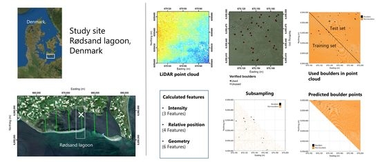
2. Study Site
3. Materials and Methods
3.1. Surveys and Instruments
3.2. Topo-Bathymetric LiDAR Data Processing
3.3. Manual Classification of Stones on Training and Test Areas
3.4. Stone Detection Using Machine Learning
3.4.1. Features
3.4.2. Random Forest Automatic Stone Detection
3.4.3. Performance and Accuracy Assessment
4. Results
4.1. Manually Classified Boulder Points
4.2. Features in the Training and Test Set
4.2.1. Boulder Density and Size—Subsampling and Radius
4.2.2. Feature Selection
4.3. Boulder Prediction Using Random Forest
4.4. Performance and Accuracy Assessment
5. Discussion
5.1. Evaluation of Methods to Identify Boulders and Verified Boulder Points
5.2. Evaluation of Selected Training Area
5.3. Prediction Errors and Possible Algorithm Improvements
5.4. Performance Evaluation
5.5. Processing Time and Upscaling
5.6. Boulder Dynamics
6. Conclusions
Author Contributions
Funding
Institutional Review Board Statement
Informed Consent Statement
Data Availability Statement
Acknowledgments
Conflicts of Interest
References
- Al-Hamdani, Z.; Jensen, J.B.; Skar, S.; Nørgaard-Pedersen, N.; Leth, J.O.; Lomholt, S.; Bennike, O.; Granat, H.; Andersen, M.S.; Rödel, L.G.; et al. Marin Habitatkortlægning I De Indre Danske Farvande; Naturstyrelsen: Copenhagen, Denmark, 2014. (In Danish) [Google Scholar]
- Al-Hamdani, Z.; Skar, S.; Jensen, J.B.; Rödel, L.G.; Pjetursson, B.; Bennike, O.; Oxfeldt Jensen, G.C.; Rasmussen, M.B.; Dahl, K.; Koefoed Rømer, J.; et al. Marin Habitatkortlægning i Skagerrak og Nordsøen 2015; Naturstyrelsen: Copenhagen, Denmark, 2015. (In Danish) [Google Scholar]
- Al-Hamdani, Z.; Owen, M.; Rödel, L.G.; Witt, N.; Nørgaard-Petersen, N.; Bennike, O.; Sabra, H.; Eriksen, L.N.; Kragh, S.; Jensen, J.B.; et al. Kortlægning af Natura 2000-Områder Marin Habitatkortlægning i Skagerrak Og Nordsøen 2017–2018; Miljøstyrelsen: Copenhagen, Denmark, 2019; ISBN 978-87-7038-027-0. (In Danish) [Google Scholar]
- Al-Hamdani, Z. Analyse af 1170 Stenrev Henholdsvis Indenfor og Udenfor Marine Habitatområder; GEUS: Århus, Denmark, 2018. (In Danish) [Google Scholar]
- Al-Hamdani, Z.; Skar, S. Analyse af Naturtype 1170 Stenrev Henholdsvis Indenfor og Udenfor de Marine Habitatområder; GEUS: Århus, Denmak, 2017. (In Dansih) [Google Scholar]
- Lee, H. Artificial Reefs for Ecosystem Restoration and Coastal Erosion Protection with Aquaculture and Recreational Amenities. Reef J. 2009, 1. [Google Scholar] [CrossRef]
- Dahl, K.; Lundsteen, S.; Helmig, S.A. Stenrev—Havets oaser. Danmarks Miljøundersøgelser, G.E.C. Gads Forlag. 2003. Available online: https://www2.dmu.dk/1_Viden/2_Publikationer/3_miljobib/rapporter/MB02.pdf (accessed on 15 August 2021). (In Danish).
- Interpretation Manual of European Union Habitats. European Commission dg Environment. Nature, ENV B.3. 2013. Available online: https://ec.europa.eu/environment/nature/legislation/habitatsdirective/docs/Int_Manual_EU28.pdf (accessed on 15 August 2021).
- Helmig, S.A.; Nielsen, M.M.; Petersen, J.K. Andre Presfaktorer end Næringsstoffer og Klimaforandringer—Vurdering af Omfanget af Stenfiskeri i Kystnære Marine Områder; DTU Aqua-rapport; DTU Aqua: Lyngby, Denmark, 2020. (In Danish) [Google Scholar]
- Al-Hamdani, Z.; Jensen, J.B.; Nørgaard-Pedersen, N.; Skar, S.; Rödel, L.G.; Paradeisis-Stathis, S. Investigating the Potential of Stone Reefs in Reducing Nutrient Loads, as an Input to There-Establishing of a Stone Reef in the Natura 2000-Area “Løgstør Bredning, Vejlerne and Bulbjerg”; GEUS: Århus, Denmark, 2016. [Google Scholar]
- Greene, A.; Rahman, A.F.; Kline, R.; Rahman, M.S. Side scan sonar: A cost-efficient alternative method for measuring seagrass cover in shallow environments. Estuar. Coast. Shelf Sci. 2018, 207, 250–258. [Google Scholar] [CrossRef]
- Mandlburger, G. A review of airborne laser bathymetry for mapping of inland and coastal waters. Hydrogr. Nachr. 2020, 6–15. [Google Scholar] [CrossRef]
- Maas, H.; Mader, D.; Richter, K.; Westfeld, P. Improvements in LiDAR bathymetry data analysis. Int. Arch. Photogramm. Remote Sens. Spat. Inf. Sci. 2019, XLII-2/W10, 113–117. [Google Scholar] [CrossRef] [Green Version]
- Andersen, M.S.; Gergely, Á.; Al-Hamdani, Z.K.; Steinbacher, F.; Larsen, L.R.; Ernstsen, V.B. Processing and performance of topobathymetric lidar data for geomorphometric and morphological classification in a high-energy tidal environment. Hydrol. Earth Syst. Sci. 2017, 21, 43–63. [Google Scholar] [CrossRef] [Green Version]
- Agrafiotis, P.; Karantzalos, K.; Georgopoulos, A.; Skarlatos, D. Correcting Image Refraction: Towards Accurate Aerial Image-Based Bathymetry Mapping in Shallow Waters. Remote Sens. 2020, 12, 322. [Google Scholar] [CrossRef] [Green Version]
- Sagawa, T.; Yamashita, Y.; Okumura, T.; Yamanokuchi, T. Satellite Derived Bathymetry Using Machine Learning and Multi-Temporal Satellite Images. Remote Sens. 2019, 11, 1155. [Google Scholar] [CrossRef] [Green Version]
- Yu, L.; Liang, L.; Wang, J.; Zhao, Y.; Cheng, Q.; Hu, L.; Liu, S.; Yu, L.; Wang, X.; Zhu, P.; et al. Meta-discoveries from a synthesis of satellite-based land-cover mapping research. Int. J. Remote. Sens. 2014, 35, 4573–4588. [Google Scholar] [CrossRef]
- Murdoch, W.J.; Singh, C.; Kumbier, K.; Abbasi-Asl, R.; Yu, B. Definitions, methods, and applications in interpretable machine learning. Proc. Natl. Acad. Sci. USA 2019, 116, 22071–22080. [Google Scholar] [CrossRef] [Green Version]
- Yan, W.Y.; Shaker, A.; El-Ashmawy, N. Urban land cover classification using airborne LiDAR data: A review. Remote Sens. Environ. 2015, 158, 295–310. [Google Scholar] [CrossRef]
- Janowski, L.; Trzcinska, K.; Tegowski, J.; Kruss, A.; Rucinska-Zjadacz, M.; Pocwiardowski, P. Nearshore Benthic Habitat Mapping Based on Multi-Frequency, Multibeam Echosounder Data Using a Combined Object-Based Approach: A Case Study from the Rowy Site in the Southern Baltic Sea. Remote Sens. 2018, 10, 1983. [Google Scholar] [CrossRef] [Green Version]
- Janowski, Ł.; Wróblewski, R.; Dworniczak, J.; Kolakowski, M.; Rogowska, K.; Wojcik, M.; Gajewski, J. Offshore benthic habitat mapping based on object-based image analysis and geomorphometric approach. A case study from the Slupsk Bank, Southern Baltic Sea. Sci. Total. Environ. 2021, 801, 149712. [Google Scholar] [CrossRef]
- Papenmeier, S.; Hass, H.C. Detection of Stones in Marine Habitats Combining Simultaneous Hydroacoustic Surveys. Geosciences 2018, 8, 279. [Google Scholar] [CrossRef] [Green Version]
- Held, P.; Deimling, J.S.V. New Feature Classes for Acoustic Habitat Mapping—A Multibeam Echosounder Point Cloud Analysis for Mapping Submerged Aquatic Vegetation (SAV). Geosciences 2019, 9, 235. [Google Scholar] [CrossRef] [Green Version]
- Oshiro, T.M.; Perez, P.S.; Baranauskas, J.A. How Many Trees in a Random Forest? In Machine Learning and Data Mining in Pattern Recognition. MLDM 2012. Lecture Notes in Computer Science; Perner, P., Ed.; Springer: Berlin, Heidelberg, 2012; Volume 7376. [Google Scholar] [CrossRef]
- Lowell, K.; Calder, B. Extracting Shallow-Water Bathymetry from Lidar Point Clouds Using Pulse Attribute Data: Merging Density-Based and Machine Learning Approaches. Mar. Geod. 2021, 44, 259–286. [Google Scholar] [CrossRef]
- Mandlburger, G.; Pfennigbauer, M.; Schwarz, R.; Flöry, S.; Nussbaumer, L. Concept and Performance Evaluation of a Novel UAV-Borne Topo-Bathymetric LiDAR Sensor. Remote Sens. 2020, 12, 986. [Google Scholar] [CrossRef] [Green Version]
- Collin, A.; Archambault, P.; Long, B. Predicting species diversity of benthic communities within turbid nearshore using full-waveform bathymetric LiDAR and machine learners. PLoS ONE 2011, 6, e21265. [Google Scholar] [CrossRef] [PubMed] [Green Version]
- Kogut, T.; Weistock, M.; Bakuła, K. Classification of data from airborne lidar bathymetry with random forest algorithm based on different feature vectors. Isprs—Int. Arch. Photogramm. Remote Sens. Spat. Inf. Sci. 2019, XLII-2/W16, 143–148. [Google Scholar] [CrossRef] [Green Version]
- Forsberg, P.L.; Lumborg, U.; Bundgaard, K.; Ernstsen, V.B. Impact of mussel bioengineering on fine-grained sediment dynamics in a coastal lagoon: A numerical modelling investigation. J. Mar. Syst. 2017, 176, 1–12. [Google Scholar] [CrossRef]
- Forsberg, P.; Lumborg, U.; Andersen, T.; Kroon, A.; Ernstsen, V. The relative impact of future storminess versus offshore dredging on suspended sediment concentration in a shallow coastal embayment: Rødsand lagoon, western Baltic Sea. Ocean Dyn. 2019, 69, 1–13. [Google Scholar] [CrossRef]
- Ries, O.; Drønen, N.; Kroon, A. Barrier morphodynamics under micro-tidal and low to moderate wave conditions, Rødsand, Denmark. Dynamics 2017, 1090–1098. [Google Scholar]
- FEHY. Fehmarnbelt Fixed Link EIA. Marine Soil—Baseline. In Coastal Morphology along Fehmarn and Lolland; Raport no. E1TR0056—2013; FEHY Consortium/Co DHI: Hørsholm, Denmark, 2013; Volume III, p. 212. ISBN 978-87-92416-34-6. [Google Scholar]
- DHI. Rødsand 2. Waves and Sediment Transport. Littoral Transport and Coastal Morphology; Final Rapport prepared for Dong Energy; DHI: Hørsholm, Denmark, 2007. [Google Scholar]
- Forsberg, P.L.; Ernstsen, V.B.; Andersen, T.J.; Winter, C.; Becker, M.; Kroon, A. The effect of successive storm events and seagrass coverage on sediment suspension in a coastal lagoon. Estuarine. Coast. Shelf Sci. 2018, 212, 329–340. [Google Scholar] [CrossRef]
- FEMA. Fehmarnbelt Fixed Link EIA. Marine Fauna and Flora—Baseline; Habitat Mapping of the Fehmarnbelt Area Report No. E2TR0020; FEMA Consortium/Co DHI: Hørsholm, Denmark, 2013; Volume III, p. 109. [Google Scholar]
- Riegl: LASextrabytes implementation in RIEGL software—Whitepaper, Riegl Laser Measurement Systems GmbH. Available online: http://www.riegl.com/uploads/tx_pxpriegldownloads/Whitepaper_LAS_extrabytes_implementation_in_RIEGL_Software_2019-04-15.pdf (accessed on 15 May 2021).
- Kumpumäki, T. Lasdata. 2021. Available online: https://www.mathworks.com/matlabcentral/fileexchange/48073-lasdata (accessed on 19 May 2020).
- Beksi, W. Estimate Surface Normals. Available online: https://www.mathworks.com/matlabcentral/fileexchange/46757-estimate-surface-normals (accessed on 8 June 2020).
- Höfle, B.; Vetter, M.; Pfeifer, N.; Mandlburger, G.; Stötter, J. Water surface mapping from airborne laser scanning using signal intensity and elevation data. Earth Surf. Process. Landf. 2009, 34, 1635–1649. [Google Scholar] [CrossRef]
- MathWorks. Computer Vision Toolbox (R2021a). Available online: https://se.mathworks.com/help/vision/index.html?s_tid=CRUX_lftnav (accessed on 15 May 2020).
- Bi, C.; Yang, L.; Duan, Y.; Shi, Y. A survey on visualization of tensor field. J. Vis. 2019, 22, 641–660. [Google Scholar] [CrossRef]
- Lin, C.; Chen, J.; Su, P.L.; Chen, C. Eigen-feature analysis of weighted covariance matrices for LiDAR point cloud classification. Isprs J. Photogramm. Remote Sens. 2014, 94, 70–79. [Google Scholar] [CrossRef]
- Qin, X.; Wu, G.; Lei, J.; Fan, F.; Ye, X.; Mei, Q. A Novel Method of Autonomous Inspection for Transmission Line based on Cable Inspection Robot LiDAR Data. Sensors 2018, 18, 596. [Google Scholar] [CrossRef] [PubMed] [Green Version]
- Breiman, L. Random Forests. Mach. Learn. 2001, 45, 5–32. [Google Scholar] [CrossRef] [Green Version]
- MathWorks. Statistics and Machine Learning Toolbox (R2021a). 2021. Available online: https://se.mathworks.com/help/stats/index.html?s_tid=CRUX_lftnav (accessed on 15 May 2020).
- Loh, W.; Shih, Y. Split selection methods for classification trees. Stat. Sin. 1997, 7, 815–840. [Google Scholar]
- Chen, C. Using Random Forest to Learn Imbalanced Data; Department of Statistics, UC Berkley: Berkeley, CA, USA, 2004. [Google Scholar]
- Von Rönn, G.A.; Krämer, K.; Franz, M.; Schwarzer, K.; Reimers, H.-C.; Winter, C. Dynamics of Stone Habitats in Coastal Waters of the Southwestern Baltic Sea (Hohwacht Bay). Geosciences 2021, 11, 171. [Google Scholar] [CrossRef]
- Misiuk, B.; Diesing, M.; Aitken, A.; Brown, C.J.; Edinger, E.N.; Bell, T. A Spatially Explicit Comparison of Quantitative and Categorical Modelling Approaches for Mapping Seabed Sediments Using Random Forest. Geosciences 2019, 9, 254. [Google Scholar] [CrossRef] [Green Version]
- Report from the commission to the council and the european parliament The first phase of implementation of the Marine Strategy Framework Directive (2008/56/EC) The European Commission’s assessment and guidance/*COM/2014/097 final*. Available online: https://eur-lex.europa.eu/legal-content/EN/TXT/?uri=celex%3A52014DC0097 (accessed on 15 August 2021).
- Schwarzer, K.; Bohling, B.; Heinrich, C. Submarine hard-bottom substrates in the western Baltic Sea—human impact versus natural development. J. Coast. Res. Spec. Issue 2014, 145–150. [Google Scholar] [CrossRef]
- Torn, K.; Peterson, A.; Herkül, K. Predicting the Impact of Climate Change on the Distribution of the Key Habitat-Forming Species in the Ne Baltic Sea. J. Coast. Res. 2020, 95, 177–181. [Google Scholar] [CrossRef]


| Year | Quality | Pixel Uncertainty (m) | Georeferencing Uncertainty (m) | Buffer Zone (m) | Used |
|---|---|---|---|---|---|
| 2019 | + | 0.10 | 0 (reference) | 0.20 | Yes |
| 2018 | + | 0.10 | 0.12 | 0.32 | Yes |
| 2017 | + | 0.10 | 0.30 | 0.50 | Yes |
| 2016 | + | 0.10 | 0.35 | 0.55 | Yes |
| 2015 | + | 0.10 | 1.40 | 1.60 | Yes |
| 2013 | + | 0.10 | 1.40 | 1.60 | Yes |
| 2010 | − | 0.10–0.20 | − | − | No |
| 2008 | + | 0.10–0.20 | 1.40 | 1.60 | Yes |
| 2006 | + | 0.10–0.40 | 1.80 | 2.00 | Yes |
| 2002 | − | 0.40 | − | − | No |
| 1999 | − | 0.40 | − | − | No |
| 1995 | − | 0.80 | − | − | No |
| 1954 | + | 0.25 | 9.60 | 9.80 | No |
| Features | Radius 0.5 m | Radius 1.0 m | Radius 2.0 m | Radius 3.0 m | Single Value |
|---|---|---|---|---|---|
| Spectral features | - | - | - | - | - |
| Intensity | - | - | - | - | x |
| Std intensity | x | x | x | x | - |
| Mean Intensity | x | x | x | x | - |
| Relative position features | - | - | - | - | - |
| z | - | - | - | - | x |
| Std z | x | x | x | x | - |
| Mean z | x | x | x | x | - |
| dz | x | x | x | x | - |
| dp | - | x | x | x | - |
| Covariance features | - | - | - | - | - |
| Linearity | x | - | - | - | - |
| Planarity | x | - | - | - | - |
| Sphericity | x | - | - | - | - |
| Omnivariance | x | - | - | - | - |
| Anisotropy | x | - | - | - | - |
| Change of curvature | x | - | - | - | - |
| Neighborhood Radius Size (m) | Points in Neighborhood Minimum | Points in Neighborhood Maximum | Points in Neighborhood Average | Points Excluded (%) |
|---|---|---|---|---|
| 0.5 | 4 | 23 | 10 | 0.23 |
| 1.0 | 4 | 46 | 19 | 0.002 |
| 2.0 | 6 | 91 | 34 | 0 |
| 3.0 | 8 | 134 | 50 | 0 |
| Radius (m) | Subsampling /Cost | Predictor Selection | P (%) | R (%) | F-Score (%) | TPR (%) | TNR (%) | G-Mean (%) | Acc (%) | W-Acc (%) | Balanced Acc (%) | Cohen’s Kappa |
|---|---|---|---|---|---|---|---|---|---|---|---|---|
| 0.5 | 1:7/7:1 | Curvature | 32 | 23 | 27 | 23 | 100 | 48 | 99 | 33 | 62 | 0.27 |
| 0.5 and 2.0 | 1:10/10:1 | Curvature | 36 | 22 | 27 | 22 | 100 | 46 | 99 | 29 | 61 | 0.27 |
| Radius (m) | Subsampling/Cost | Predictor Selection | R (%) | P (%) | F-Score (%) | I | S | T |
|---|---|---|---|---|---|---|---|---|
| 0.5 | 1:7/7:1 | Curvature | 57 | 27 | 37 | 12 | 44 | 21 |
| 0.5 and 2.0 | 1:10/10:1 | Curvature | 43 | 21 | 28 | 9 | 43 | 21 |
Publisher’s Note: MDPI stays neutral with regard to jurisdictional claims in published maps and institutional affiliations. |
© 2021 by the authors. Licensee MDPI, Basel, Switzerland. This article is an open access article distributed under the terms and conditions of the Creative Commons Attribution (CC BY) license (https://creativecommons.org/licenses/by/4.0/).
Share and Cite
Hansen, S.S.; Ernstsen, V.B.; Andersen, M.S.; Al-Hamdani, Z.; Baran, R.; Niederwieser, M.; Steinbacher, F.; Kroon, A. Classification of Boulders in Coastal Environments Using Random Forest Machine Learning on Topo-Bathymetric LiDAR Data. Remote Sens. 2021, 13, 4101. https://doi.org/10.3390/rs13204101
Hansen SS, Ernstsen VB, Andersen MS, Al-Hamdani Z, Baran R, Niederwieser M, Steinbacher F, Kroon A. Classification of Boulders in Coastal Environments Using Random Forest Machine Learning on Topo-Bathymetric LiDAR Data. Remote Sensing. 2021; 13(20):4101. https://doi.org/10.3390/rs13204101
Chicago/Turabian StyleHansen, Signe Schilling, Verner Brandbyge Ernstsen, Mikkel Skovgaard Andersen, Zyad Al-Hamdani, Ramona Baran, Manfred Niederwieser, Frank Steinbacher, and Aart Kroon. 2021. "Classification of Boulders in Coastal Environments Using Random Forest Machine Learning on Topo-Bathymetric LiDAR Data" Remote Sensing 13, no. 20: 4101. https://doi.org/10.3390/rs13204101