Remote-Sensing-Based Streamflow Forecasting Using Artificial Neural Network and Support Vector Machine Models

Abstract

In this study, we aimed to investigate the hydrological performance of three gridded precipitation products—CHIRPS, RFE, and TRMM3B42V7—in monthly streamflow forecasting. After statistical evaluation, two monthly streamflow forecasting models—support vector machine (SVM) and artificial neural network (ANN)—were developed using the monthly temporal resolution data derived from these products. The hydrological performance of the developed forecasting models was then evaluated using several statistical indices, including NSE, MAE, RMSE, and R². The performance measures confirmed that the CHIRPS product has superior performance compared to RFE 2.0 and TRMM data, and it could provide reliable rainfall estimates for use as input in forecasting models. Likewise, the results of the forecasting models confirmed that the ANN and SVM both achieved acceptable levels of accuracy for forecasting streamflow; however, the ANN model was superior (R² = 0.898–0.735) to the SVM (R² = 0.742–0.635) in both the training and testing periods.

1. Introduction

Reliable streamflow forecasting is a topic of concern in hydrological studies for the operation of flood and drought mitigation systems and the operation and planning of reservoirs [1,2,3]. In this regard, numerous attitudes and models have been applied to improve the modeling and simulation of streamflow forecasting [4,5,6,7,8]. The existing models that are commonly used in hydrological applications are typically classified into two main groups, namely physical and data-driven models. Complicated mathematical tools and extensive expertise are required to work with the physical-based models, which are sophisticated and require a large amount of calibration data [8]. Data-driven models can forecast streamflow with appropriate accuracy and rely on the physics of hydrological problems as their key feature [9]. In recent decades, rising trends in computing capability and data availability have made the development of data-driven models more attractive and beneficial [10,11,12]. Multilinear regression (MLR) is recognized as performing quite well for long-term forecasting, and it is one of the typical forms of data-driven models [13]. In MLR, the function that relates input and output records is linear, whereas streamflow forecasting relies on both known and unknown variables, thus rendering it an extremely nonlinear process.

Numerous studies recently confirmed the reliability of SVM as a machine learning model and ANN as an artificial intelligence approach in modeling the significant non-linearity between parameters in hydrological applications, including rainfall–runoff models, groundwater simulation, streamflow prediction, and flood prediction [12,14,15,16,17,18,19,20,21,22,23,24,25,26]. The potential of such hydrological applications mainly relies on the spatiotemporal resolution and consistency of accurate long-term rainfall series. Although rainfall datasets are available in different formats, researchers are mostly attracted to standard or ground-based weather stations. Ground-based rainfall networks have irregular spatiotemporal distribution in some regions, which results in poor hydrological simulation and inadequate solutions to issues related to water resources, highlighting the importance of using satellite-based and global precipitation products [27,28,29]. These products are being significantly improved, allowing for estimates of these products to evolve as a reliable source of data with considerable spatiotemporal accuracy, and they could become reasonable alternatives to recovering unavailable rain gauge data, particularly in regions with no robust network of ground rain gauges [30,31].

Due to the inaccuracies existing in satellite datasets and uncertainties arising from sampling technologies, the regional variation in the capabilities of grid precipitation products is quite considerable [32]. In the past three decades, numerous studies have investigated the potential of various satellite products. Javanmard et al. [27] evaluated TRMM_3B42 products over Iran and seasonal and annual timescales against ground records, reporting that they preserved the spatiotemporal rainfall patterns but had limitations in reliably retrieving the rainfall quantity. Ahmed et al. [33] assessed two satellite products, RFE and TRMM, finding that the two products perform well in estimating and observing rainfall. Sulugodu et al. [34] evaluated the hydrological performance of CHIRPS in streamflow forecasting, and they found that satellite-derived products showed suitable accuracy. The key point taken from the previous literature was that at both the global and regional scales, no satellite product could satisfy all verification measurements or be effectively implemented in several hydrological applications [35,36,37,38].

In this study, we attempted to: (1) examine the potential of three commonly used precipitation products with high temporal and spatial resolution, namely Climate Hazards Group Infra-Red Precipitation with Station (CHIRPS, https://developers.google.com/earth-engine/datasets (access on 12 July 2020)), African Rainfall Climatology (RFE 2.0, https://journals.ametsoc.org (access on 12 July 2020)), and Tropical Rainfall Measuring Mission (TRMM-3B42V7, https://climatedataguide.ucar.edu/climate-data/trmm (access on 12 July 2020)); (2) use these products to develop a monthly streamflow forecasting model using ANN and SVM models; and (3) assess the forecasting models’ reliability. To the best of our knowledge, no studies on the application of artificial neural network fuzzy inference system and support vector machine techniques to forecast streamflow using CHIRPS, RFE, and TRMM-3B42V7 rainfall data as inputs in the study area have been carried out to date. The structure of this paper is as follows: following this introduction, Section 2 comprises a detailed methodology and the components of the proposed models. Section 3 presents a detailed comparison between historical rainfall records and satellite product estimates, the case study results, a discussion of ANN- and SVM-based forecasts, and their applications in streamflow forecasting. Finally, a discussion and concluding remarks are presented in Section 4 and Section 5, respectively.

2. Materials and Methods

2.1. Case Study

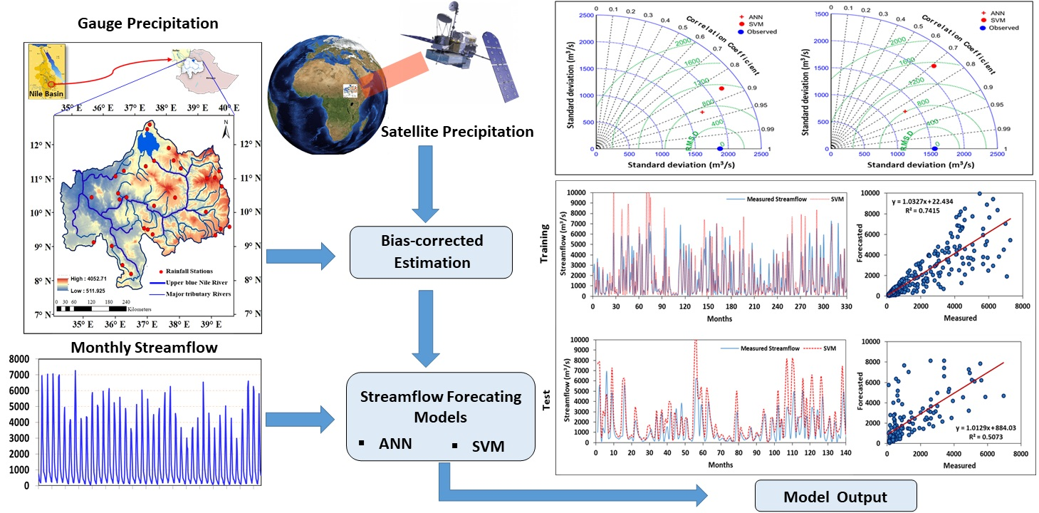
The approach we propose herein was implemented in the UBNRB, which is situated in Western Ethiopia, extends between 7°45′ and 12°45′N and from 34°05′ to 39°45′E, and has an area coverage of about 200,000 km² (Figure 1). The Blue Nile originates at elevations of about 3000 m; then, it flows 1450 km from its origin at an elevation of 1829 m to reach Sudan with an elevation of 490 m, merging with the White Nile to form the Nile [38] (Figure 1). The river and its substreams have a natural northwest slope in general, but they are steeper in the east than in the west and northeast. During the primary rain season, June–October, almost 84% of the overall rainfall volume is received. On the Sudan–Ethiopia border, the estimated annual streamflow is around 48.660 million m³, exceeding 40% of the overall water resources in Ethiopia. The average annual runoff over the UBNRB is about 46 billion m³ (1456 m³/s), with a runoff ratio of 18% [39]. The rivers of the basin provide the Nile with more than 62% of its overall discharge at Aswan; therefore, the UBNRB is a major and vital water resource for Ethiopia and downstream countries.

2.2. Data Collection

2.2.1. Ground Data

Fifty years (1964–2014) of monthly rainfall records from 30 meteorological stations (Figure 1), representing suitable spatial distribution across the UBNRB, were included with an average annual rainfall of 1260 mm, which is relatively higher than that of other sub-basins [40]. The climatic seasons of the UBNRB include the dry season in October–February (Bega), a relatively short raining season in March–May (Belg), and a long raining season in June–September (Kiremt), during which about 74% of rainfall is received. The rainfall distribution over the UBNRB is characterized by significant diversity both spatially (as it decreases spatially from the southwest to the east and northeast) and temporally over the year. The streamflow datasets considered in this study were the monthly streamflow records of the UBNRB measured at El-Diem station (1966–2008), located near the Ethiopia–Sudan border (Figure 1).

2.2.2. Gridded Precipitation Datasets

The accuracy and performance of three precipitation products—CHIRPS, RFE2, and TRMM-3B42V7—were evaluated at a monthly scale.

Table 1. Summary of the three gridded precipitation datasets used in this study.

Product	Start	End	Resolution		Coverage
			Spatial	Temporal
CHIRPS	1981	Present	0.25°	Daily	50°N to 50°S
REF 2.0	1998	Present	0.10°	Daily	40″S to 40″N
TRMM-3B42V7	1998	Present	0.25°	Daily	50°N to 50°S

briefly illustrates the investigated products and their spatiotemporal characteristics.

CHIRPS Dataset

Since 1981, CHIRPS has been available in a range of high-resolution formats and with time scales varying from daily to monthly [41]. Version 2 of the NOAA Climate Prediction System (CFS) atmospheric model rainfall area, TRMM-3B42V7, a precipitation climate dataset (CHPclim), and rainfall station records were used to build CHIRPS. CHIRPS covers a range from 50°S to 50°N with spatial resolutions of 0.05° and 0.25° for all longitudes. In this research, the 0.25° resolution dataset was analyzed and evaluated. CHIRPS version 2 is accessible to the public for download from (http://chg.geog.ucsb.edu/data/chirps, accessed on 11 October 2021).

TRMM-3B42V7 Dataset

The TRMM product was initially issued in 1997 as a cooperative space mission by the Japanese NASDA and NASA for monitoring and analyzing tropical and subtropical precipitation, as well as to provide a precise estimation of quasi-worldwide precipitation [42,43]. Since it was introduced in 1997, TRMM-3B42V7 has provided beneficial precipitation data for a quasi-global range from 50°N to 50°S with a 0.25° spatial resolution.

RFE 2.0 Dataset

The RFE product was originally released and implemented as an operational product in 1998 by CPC/NOAA; it covers a range from 40°S to 40°N and from 20°W to 55°E, and it is spatially distributed at 0.1° [29]. The RFE datasets rely on the aggregation of daily measured rainfall records from the Global Telecommunication System (GTS), along with advanced microwave sounding unit and special sensor microwave estimates of satellite rainfall. Version 2 of RFE became usable at the beginning of 2001 and originally worked to estimate rainfall on the African continent; it was eventually enhanced to include other areas [30].

2.3. Methodology

2.3.1. Performance Evaluation of Precipitation Datasets

Substantial post-processing dataset bias correction, assessment, and validations are performed before implementing the output of the precipitation products’ data in streamflow forecasting. The procedure of gridded precipitation assessment could be performed either by (1) precise comparisons with gauge records or (2) employing hydrological models and evaluating the capabilities of the products in simulating streamflow. The first technique was employed in this study to assess the investigated precipitation products before using their data as input for the forecasting models. The accuracy of these products was evaluated based on the coefficient of correlation (Cr), RMSE, ME, and relative bias (BIAS), respectively, as follows:

$${\mathrm{C}}_{\mathrm{r}}=\frac{{{\displaystyle \sum }}_{\mathrm{i}=1}^{\mathrm{n}}\left({\mathrm{G}}_{\mathrm{i}}-\bar{\mathrm{G}}\right)\left({\mathrm{S}}_{\mathrm{i}} - \bar{\mathrm{S}}\right)}{\sqrt{{{\displaystyle \sum }}_{\mathrm{i}=1}^{\mathrm{n}}{\left({\mathrm{G}}_{\mathrm{i}}- \bar{\mathrm{G}}\right)}^2\sqrt{{{\displaystyle \sum }}_{\mathrm{i}=1}^{\mathrm{n}}{\left({\mathrm{S}}_{\mathrm{i}}- \bar{\mathrm{S}}\right)}^2}}}$$

(1)

$$\mathrm{ME}=\frac{{{\displaystyle \sum }}_{\mathrm{i}=1}^{\mathrm{n}}\left({\mathrm{S}}_{\mathrm{i}}-{\mathrm{G}}_{\mathrm{i}}\right)}{\mathrm{n}}\ast 100\%$$

(2)

$$\mathrm{RMSE}=\sqrt{\frac{1}{\mathrm{n}}{\displaystyle \sum }_{\mathrm{i}=1}^{\mathrm{n}}{\left({\mathrm{S}}_{\mathrm{i}}-{\mathrm{G}}_{\mathrm{i}}\right)}^2}$$

(3)

$$\mathrm{Bias}=\frac{{{\displaystyle \sum }}_{\mathrm{i}=1}^{\mathrm{n}}{\mathrm{S}}_{\mathrm{i}}-{\mathrm{G}}_{\mathrm{i}}}{{{\displaystyle \sum }}_{\mathrm{i}=1}^{\mathrm{n}}{\mathrm{G}}_{\mathrm{i}}}\ast 100$$

(4)

where i and j are the grid points; n is the number of samples; and G and S are the gauge records and satellite estimations, respectively.

Contingency scores, which reflect the extent of correlation between the satellite estimates and recorded rainfall, were also calculated utilizing the number of hits, false alarms (FARs), and misses (Equations (5)–(7)). The probability of detection (POD), often referred to as the hit rate, represents the percentage of events encountered that the precipitation product assessed that was correctly estimated on the basis of the threshold limits. The FAR provides the magnitude of false alarms that were provided by the products and were not eventually detected. Then, by employing the critical success index (CSI), the hit rate and false alarm percentages are integrated into a single score that indicates the performance evaluation of the cumulative rainfall detection of the precipitation products compared to the recorded rainfall. For the POD and CSI, the ratings vary from 0 to 1 for the weak and strong ends, respectively, and for FAR, the ratings vary from 1 to 0 for the weak and strong ends, respectively.

$$\mathrm{Hit}={{\displaystyle \sum }}_{\mathrm{i}=1}^{\mathrm{n}}\left({\mathrm{S}}_{\mathrm{i}}-{\mathrm{G}}_{\mathrm{i}}\right) \mathrm{when} {\mathrm{S}}_{\mathrm{i}} > 0 \mathrm{and} {\mathrm{G}}_{\mathrm{i}} > 0$$

(5)

$$\mathrm{Miss}={{\displaystyle \sum }}_{\mathrm{i}=1}^{\mathrm{n}}\left({\mathrm{S}}_{\mathrm{i}}-{\mathrm{G}}_{\mathrm{i}}\right) \mathrm{when} {\mathrm{S}}_{\mathrm{i}}=0 \mathrm{and} {\mathrm{G}}_{\mathrm{i}} > 0$$

(6)

$$\mathrm{False}={{\displaystyle \sum }}_{\mathrm{i}=1}^{\mathrm{n}}\left({\mathrm{S}}_{\mathrm{i}}-{\mathrm{G}}_{\mathrm{i}}\right) \mathrm{when} {\mathrm{S}}_{\mathrm{i}} > 0 \mathrm{and} {\mathrm{G}}_{\mathrm{i}} =0$$

(7)

$$\mathrm{POD}=\frac{{\mathrm{N}}_{\mathrm{hit}}}{{\mathrm{N}}_{\mathrm{hit}}+{\mathrm{N}}_{\mathrm{miss}}}$$

(8)

$$\mathrm{FAR}=\frac{{\mathrm{N}}_{\mathrm{false}}}{{\mathrm{N}}_{\mathrm{hit}}+{\mathrm{N}}_{\mathrm{false}}}$$

(9)

$$\mathrm{CSI}=\frac{{\mathrm{N}}_{\mathrm{hit}}}{{\mathrm{N}}_{\mathrm{hit}}+{\mathrm{N}}_{\mathrm{miss}}+{\mathrm{N}}_{\mathrm{false}}}$$

(10)

where Hit indicates precipitation identified concurrently by the satellite estimation and gauge records; Miss reflects events detected by the gauge but not identified by the satellite estimation; and False is the opposite of Miss, meaning that precipitation is detected by satellite estimation but not recorded by the gauges.

2.3.2. Forecasting Models

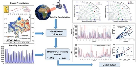
The primary aim of this research was to integrate ANN and SVM with satellite-based precipitation to forecast the monthly streamflow of the upper Blue Nile River at El Diem station. The analysis started by examining the correlation between precipitation product estimates and recorded data in order to classify stations with significant correlations. Following that, using the selected precipitation data, an ANN model was developed along with an SVM to forecast streamflow. Finally, the performance of the two established models’ was measured using various performance metrics. Figure 2 presents a schematic flowchart of the applied methodology. To execute the proposed forecasting models, the investigated dataset was randomly split into two sets: training (70%) and testing (30%). The training dataset corresponded to the data being used in the model training, and the parameters of the model were calibrated according to the error’s interpretation of the data. The testing subset was employed in the model performance evaluation.

Support Vector Machine (SVM) Model

SVM is typically a well-suited approach for the regression and prediction of hydrological time series with acceptable performance [44,45]. SVM reflects the concept of structural risk minimization (SRM), which aims to minimize a learning model’s predicted error, eliminate the issue of overfitting, and allow for improved generalization. By applying other alternative loss functions, SVM can be extended to the regression analysis of time series to convert the nonlinearity of the measured data into a superior structural feature vector and, afterwards, to apply a linear regression to the structural vector. The SVM regression function expresses the predefined input x to the specified output y as follows:

$$\mathrm{f}\left(\mathrm{x}\right)={\mathsf{\omega }}^{\mathrm{T}}\mathsf{\phi }\left(\mathrm{x}\right)+\mathrm{b}$$

(11)

where f(x) represents the SVM model’s expected value, φ(x) is the nonlinear mapping function, and ω and b are the SVM model parameters to be optimized.

The SVM optimization model for the training dataset can be described as presented in Equation (12):

$$\{\begin{array}{c}\min \mathrm{R}\left( \mathsf{\omega }, \mathsf{\xi },{ \mathsf{\xi }}^{*},\mathsf{\epsilon }\right)=\frac{1}{2}{||\mathsf{\varpi }||}^2+\mathrm{C}\left[\mathsf{\nu }\mathsf{\epsilon }+\frac{1}{\mathrm{l}}{\displaystyle \sum _{\mathrm{i}=1}^{\mathrm{l}}}\left({\mathsf{\xi }}_{\mathrm{i}}+{\mathsf{\xi }}_{\mathrm{i}}^{*}\right)\right]\\ \mathrm{subjective} \mathrm{to} : {\mathrm{y}}_{\mathrm{i}}-{\mathsf{\varpi }}^{\mathrm{T}}\mathsf{\phi }\left({\mathrm{x}}_{\mathrm{i}}\right)-\mathrm{b} \le \mathsf{\epsilon }+{\mathsf{\xi }}_{\mathrm{i}}\\ {\mathsf{\varpi }}^{\mathrm{T}}\mathsf{\phi }\left({\mathrm{x}}_{\mathrm{i}}\right)+\mathrm{b}-{\mathrm{y}}_{\mathrm{i}} \le \mathsf{\epsilon }+{\mathsf{\xi }}_{\mathrm{i}}\\ {\mathsf{\xi }}_{\mathrm{i}}, \mathsf{\epsilon } \mathsf{\ge }0\end{array}$$

(12)

where C is the variable utilized to balance the empirical risk and complexity term of the model ${\left|\right|\mathsf{\varpi }\left|\right|}^2$ and ${\mathsf{\xi }}_{\mathrm{i}}^{*}$ is the slack variable representing the distance of the ith sample from the $\mathsf{\epsilon }$ tube. This problem can be solved as a regular nonlinear optimization problem by developing a dual optimization problem following the Lagrange multipliers approach:

$$\{\begin{array}{c}\max \mathrm{R}\left({\mathrm{a}}_{\mathrm{i}},{\mathrm{a}}_{\mathrm{i}}^{*}\right)={\displaystyle \sum _{\mathrm{i}=\mathrm{1}}^{\mathrm{l}}}\left({\mathrm{a}}_{\mathrm{i}}^{*}-{\mathrm{a}}_{\mathrm{i}}\right)-\frac{1}{2}{\displaystyle \sum _{\mathrm{i}=1}^{\mathrm{l}}}{\displaystyle \sum _{\mathrm{j}=1}^{\mathrm{l}}}\left({\mathrm{a}}_{\mathrm{i}}-{\mathrm{a}}_{\mathrm{i}}^{*}\right)\left({\mathrm{a}}_{\mathrm{j}}-{\mathrm{a}}_{\mathrm{j}}^{*}\right)\mathrm{K}\left({\mathrm{x}}_{\mathrm{i}},{\mathrm{x}}_{\mathrm{j}}\right)\\ \mathrm{subjective\; to}:{\displaystyle \sum _{\mathrm{i}=1}^{\mathrm{l}}}\left({\mathrm{a}}_{\mathrm{i}}-{\mathrm{a}}_{\mathrm{i}}^{*}\right)=0\\ 0\le {\mathrm{a}}^{\mathrm{i}},{\mathrm{a}}_{\mathrm{i}}^{*}\le \frac{\mathrm{C}}{\mathrm{l}}\\ {\displaystyle \sum _{\mathrm{i}=1}^{\mathrm{l}}}\left({\mathrm{a}}_{\mathrm{i}}+{\mathrm{a}}_{\mathrm{i}}^{*}\right)\le \mathrm{Cv}\end{array}$$

(13)

where $\mathrm{the}\mathrm{kernel}\mathrm{function},\mathrm{K}({\mathrm{x}}_{\mathrm{i}},{\mathrm{x}}_{\mathrm{j}}),$ satisfies the conditions of the Mercer and ${\mathrm{a}}_{\mathrm{i}}$ and ${\mathrm{a}}_{\mathrm{i}}^{*}$ are the positive Lagrange multipliers. The radial basis function (RBF) is the best kernel function, and it has been further examined in hydrological applications together with linear functions [46]. The RBF is expressed as:

$$\mathrm{K}\left(\mathrm{x},{ \mathrm{x}}_{\mathrm{i}}\right)=\exp \left(-\frac{{\left|\right|\mathrm{x}-{\mathrm{x}}_{\mathrm{i}}\left|\right|}^2}{{\mathsf{\sigma }}^2}\right)$$

(14)

The parameters of the SVM model are recognized after achieving the optimal solution of the dual optimization problem. The regression model for an unknown input vector x is then defined as follows:

$$\mathrm{f}\left(\mathrm{x}\right)={\displaystyle \sum }_{\mathrm{i}=1}^{\mathrm{l}}\left({\mathrm{a}}_{\mathrm{i}}^{*}-{ \mathrm{a}}_{\mathrm{i}}\right) \mathrm{K}\left({\mathrm{x}}_{\mathrm{i} },{ \mathrm{x}}_{\mathrm{j}}\right)+\mathrm{b}$$

(15)

Artificial Neural Network (ANN)

ANN implementations have been addressed in numerous experiments on hydrological problems [12,32,33,34,35,36]. The key benefits of ANNs include the ability to model nonlinear interactions, offering conceptual stability and robustness and ease of execution. ANN modeling considers both temporal variations in hydrological and climatic conditions and spatial variation in the catchment; therefore, ANNs have become prevalent in streamflow forecasting. An ANN model has three significant components: model configuration (parameters and architecture), input data layers, and output data layers (Figure 3). The input dataset is involved in the first layer, which is linked to the hidden layers by a set of neurons. Through the modeling process, there could be one or multiple hidden layers depending on the level of data mining. The number of optimal hidden layers and the corresponding neuron weights could be then identified through the training process using the input–output dataset. There are no universally accepted rules for specifying the optimum number of input variables, neurons, or hidden layers; however, data processing has been shown to enhance ANN models’ efficiency. There are several types of artificial neural networks that have been implemented in the literature, e.g., multi-layer perceptron (MLP), radial basis function (RBF) networks, and recurrent neural networks (RNNs).

2.3.3. Model Performance Measures

To measure the performance of the developed models, the following four statistical indicators were used:

• Nash–Sutcliffe efficiency coefficient (NSE) [47], expressed as:

  $$\mathrm{NSE}=1-\left[\frac{{{\displaystyle \sum }}_{\mathrm{i}=1}^{\mathrm{n}}{\left({ \mathrm{Qo}}_{\mathrm{i}}-{\mathrm{Q}}_{\mathrm{fi}}\right)}^2}{{{\displaystyle \sum }}_{\mathrm{i}=1}^{\mathrm{n}}{\left({\mathrm{Qo}}_{\mathrm{i}}-{\bar{\mathrm{Q}}}_{\mathrm{o}}\right)}^2}\right]$$

  (16)
• Mean absolute error (MAE), expressed as:

  $$\mathrm{MAE}=\frac{{{\displaystyle \sum }}_{\mathrm{i}=1}^{\mathrm{n}}\left|{\mathrm{Qo}}_{\mathrm{i}}-{\mathrm{Q}}_{\mathrm{fi}}\right|}{\mathrm{n}}$$

  (17)
• Root mean square error (RMSE), expressed as:

  $$\mathrm{RMSE}=\sqrt{\frac{{{\displaystyle \sum }}_{\mathrm{i}=1}^{\mathrm{n}}{\left({\mathrm{Qo}}_{\mathrm{i}}-{\mathrm{Q}}_{\mathrm{fi}}\right)}^2}{\mathrm{n}}}$$

  (18)
• The absolute variance fraction, R², is calculated as follows:

  $${ \mathrm{R}}^2=1-\frac{{{\displaystyle \sum }}_{\mathrm{i}=1}^{\mathrm{n}}{\left({\mathrm{Q}}_{\mathrm{i}}-{\mathrm{Q}}_{\mathrm{fi}}\right)}^2}{{{\displaystyle \sum }}_{\mathrm{i}=1}^{\mathrm{n}}{\left({\mathrm{Qo}}_{\mathrm{i}}\right)}^2}$$

  (19)

  where Q_o is the observed streamflow, Q_f is the predicted streamflow, ${\bar{\mathrm{Q}}}_{\mathrm{o}}$ is the average of the observed streamflow, and n is the total amount of data.

2.4. Design of Experiments for Streamflow Simulation

Design of experiments (DOE) is a tool that uses mathematical and statistical resources, allows for the understanding of particular phenomena and the factors that have an impact on a specific output of the process, and enables one to find the best set of observable parameters and experimental conditions for minimizing prediction errors and to provide optimal policies. In this study, The DOE factors were divided into two groups: forecasting models’ factors (SVM and ANN) and time series factors (precipitation and streamflow data). The DOE factors of the forecasting models included the SVM parameters (C, σ, and ε), the number of optimal hidden layers, and the corresponding neuron weights of the ANN model. The DOE factors included the correlation between the precipitation at the investigated stations and the streamflow records, as well as (consequently) the number of stations.

Based on the methods discussed above, the following steps were adopted to carry out this study (Figure 2):

▪

First of all, the analysis evaluated the quality of the investigated precipitation products against the observed rain gauge dataset at a monthly scale using visual inspection and statistical methods (Equations (1)–(10)).

▪

A linear scaling method was then applied for the purpose of bias correction. The goal of this method was to precisely match the monthly mean of corrected estimations with that of observed estimations, assuming that the rain gauge records were the true observations and the satellite estimations (TRMM-3B42 V7, RFE 2.0 and CHIRPS) were the biased estimation.

▪

To check for the presence of correlation between monthly precipitation products and the monthly streamflow, the Pearson’s coefficient was calculated to ascertain the existence of statistically significant correlations.

▪

The forecasting model (either SVM or ANN) and, consequently, the required precipitation and streamflow input data were then selected.

▪

The input datasets were split into two sets, namely training (70% of the data) and testing datasets (30% of the data).

▪

The process of model training was then performed to obtain the best evaluation parameters of each model.

▪

The selected forecasting model was then tested, and the model performance was evaluated using the evaluation criteria (Equations (16)–(19)).

▪

Finally, the historical observed monthly streamflow data were compared with the forecasted values obtained from the SVM and ANN models.

3. Results

3.1. Evaluation of Raw Satellite Estimates

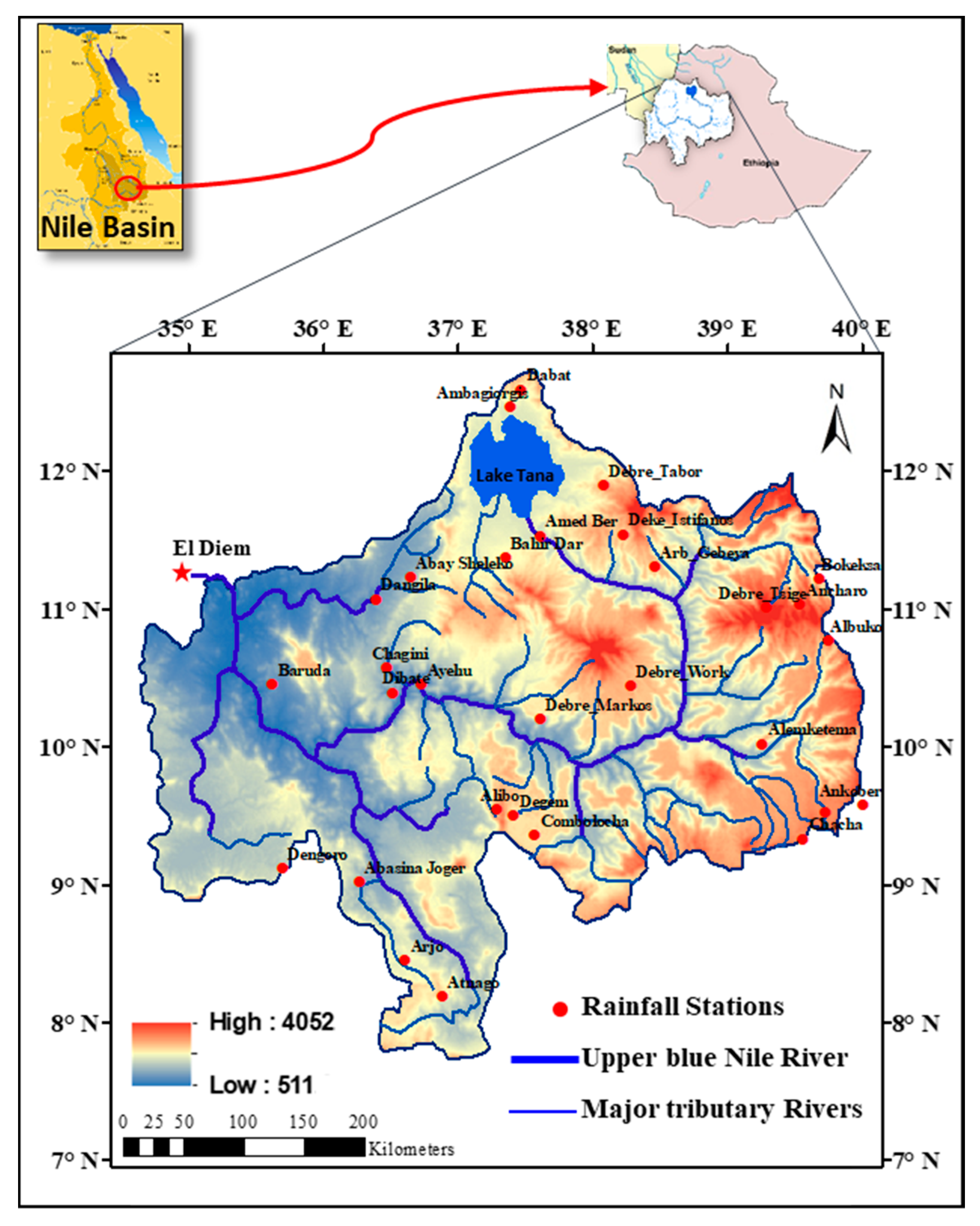
Before performing the streamflow forecasting, the reliability of the three selected precipitation products was evaluated using the data for the period of 1983–2014 for the REF dataset, 1981–2014 for the CHIRPS dataset, and 1998–2014 for the TRMM dataset. Box plots of rainfall products and measured values revealed insignificant variability in monthly rainfall quantities and trends (Figure 4 and Figure 5). The frequency of the rainfall was accurately interpreted by the three products, and the identified rainfall amounts were almost identical to the gauge records. The REF and TRMM products exceeded rainfall by a mean value of 100 mm, particularly in July and August. The estimated rainfall volumes obtained using CHIRPS were closer to the historical records; however, CHIRPS had an overall slight overestimation in rainfall volumes. Monthly rainfall estimations derived using satellite products were compared to historical data. The three products exhibited linear correlations with the measured data. CHIRPS was found to have better correlations (0.92, 0.82, 0.91, and 0.86) than the other products (

Table 2. Statistical and contingency indicators for the satellite products compared to gauge records on a monthly basis.

Station	Rainfall Sources	Cr	RMSE (mm)	ME	BIAS (%)	CSI	POD	FAR
Abasina Joger	TRMM-3B42V7	0.79	110.39	16.92	14.72	0.70	0.70	0.18
	CHIRPS	0.92	66.31	19.86	8.17	0.66	0.66	0.23
	RFE	0.75	96.54	29.80	25.93	0.68	0.68	0.21
Arjo	TRMM-3B42V7	0.72	93.01	10.77	14.53	0.62	0.62	0.28
	CHIRPS	0.82	70.02	10.77	7.88	0.60	0.60	0.30
	RFE	0.73	105.20	22.45	16.43	0.64	0.64	0.25
Bahir Dar	TRMM-3B42V7	0.81	121.62	24.88	23.14	0.58	0.58	0.32
	CHIRPS	0.91	72.63	17.32	20.22	0.54	0.54	0.37
	RFE	0.75	132.10	28.47	14.07	0.56	0.56	0.35
Combolocha	TRMM-3B42V7	0.80	92.43	14.83	10.85	0.49	0.50	0.43
	CHIRPS	0.70	154.24	29.50	21.58	0.51	0.52	0.41
	RFE	0.80	92.43	14.83	10.85	0.49	0.50	0.48

). ME and BIAS values showed that CHIRPS provided the best agreement with historical records. CHIRPS displayed superior performance in detecting rainfall occurrences, having suitable values of POD and CSI and reasonable mean FAR scores. TRMM demonstrated close to the same rain event detection performance, with around the same POD and CSI values. The statistical results achieved by comparing the monthly precipitation products with historical records demonstrated a higher level of concordance between satellite estimates and gauge records. The lowest RMSE values were scored by CHIRPS, and RFE had the highest RMSE values. The scatter plots of the monthly rainfall of the satellite products versus the gauge records are shown in Figure 6. CHIRPS demonstrated the best R² (0.85, 0.67, 0.83, and 0.74 for the Abasina Joger, Arjo, Bahir Dar, and Combolocha stations, respectively). TRMM-3B42V7 outperformed with R² = 0.55, 0.52, 0.56, and 0.64, respectively. The RFE demonstrated the smallest R².

3.2. Correlation Analysis of Rainfall and Streamflow Data

The results of the correlation analysis between the rainfall records of the investigated stations and the monthly streamflow of the upper Blue Nile River at El Diem station, at various lags at a monthly scale, revealed significant correlations. Since this study was aimed at forecasting the streamflow at a given time based on previous data on rainfall, we were mainly interested in the negative lags. Therefore, the correlation of rainfall records with streamflow was calculated at lag time t (lag 0), t-1(lag 1), and t-2 (lag 2), as shown in Figure 7. Figure 7 shows that the correlation at some stations is much closer than at others. It is evident that the rainfall of all the gauge stations at time t-1 has the strongest relationship, which is almost around 0.74 with river flow at time t. In general, all historical rainfall records and, consequently, the corresponding precipitation products in UBNRB, along with previous streamflow measurements at El Diem station, can be feasibly used as an input for ANN and SVM models to forecast streamflow. Stations with a correlation coefficient of more than 0.75 were used as inputs for the forecasting models.

3.3. SVM Model Development Using CHIRPS

The performance of SVM and ANN, in one-month-ahead streamflow forecasting, was evaluated using 13 stations as the input based on the correlation analysis. During the training phase, trial and error was used to establish the structure of the ANN and the parameters for the SVM model. The trial-and-error process for determining SVM parameters rapidly converges, whereas ANN takes longer to find the best structure for a considered dataset. Based on the literature, the radial basis function (RBF) is considered to be one of the most widely used kernel functions since it has superior predictive skill compared to other kernel functions. The SVM was developed with the use of the RBF with parameters (C, σ, and ε) for streamflow modeling, and the SVM’s performance was influenced by the parameters that were established. Since the searching parameters’ search scheme has a vital role in achieving accurate predictive performance of an SVM model, the shuffled complex evolution algorithm (SCE-UA) that has been used effectively in hydrological applications was implemented [33,34]. To obtain proper values of C, σ, and ε, the RMSE was employed to optimize the model. The results of the RBF kernel are presented in

Table 3. Performance measures of ANN and SVM models for measured and forecasted monthly streamflow.

Model	Product	Training				Test
		R2	RMSE	MAE	E	R2	RMSE	MAE	E
ANN	CHIRPS	0.898	587.289	385.732	0.913	0.735	535.322	208.193	0.809
	TRMM	-	-	-	-	0.562	1336.465	913.897	0.495
	RFE	-	-	-	-	0.437	1517.094	1018.638	0.350
SVM	CHIRPS	0.742	1125.687	638.661	0.625	0.507	1188.968	487.442	0.060
	TRMM	-	-	-	-	0.307	2431.665	1486.513	−0.67
	RFE0	-	-	-	-	0.204	2705.930	1641.719	−1.06

in terms of R², RMSE, MAE, and E. In the training period, the performance indicators were R² = 0.74, RMSE = 1125 m³/s, MAE = 638, and E = 0.625; these indicators for the testing phase were R² = 0.507, RMSE = 1188 m³/s, MAE = 487, and E = 0.06. Figure 8 shows the historical and forecasted streamflow, as well as a scatter plot for the SVM model, in the training and testing periods. A significant drop in the performance level can be observed in Figure 8 in terms of the training and testing results. The results further demonstrate that the SVM model overestimated the values of the forecasted streamflow by 37%.

3.4. ANN Model Development Using CHIRPS

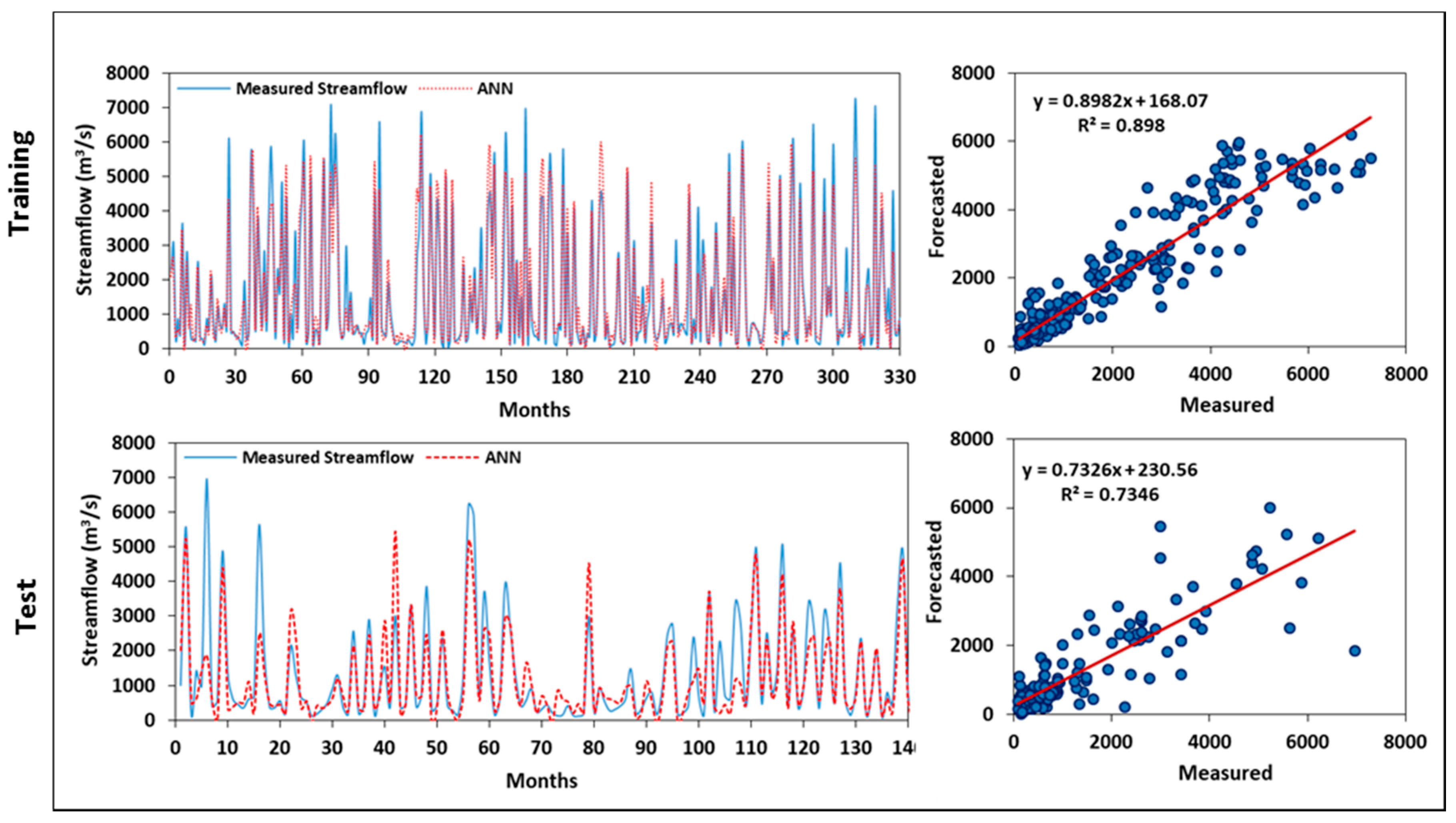
The three-layer ANN model was used on the basis of the back-propagation training system, the sigmoid activation function was used by hidden nodes, and the layer of the output employed the linear function. Since the number of nodes within the hidden layer of the developed ANN model was known to have a significant impact on the model’s performance, the optimal number of neurons in this layer was determined through a trial-and-error approach by changing the number of neurons between 1 and 20. The process of training ended when the RMSE of all testing datasets reached the minimum. The best performance in the testing period was achieved when there were eight nodes in the hidden layer; therefore, the number of hidden nodes was adjusted to eight. The performance indicators in the training phase were R² = 0.898, RMSE = 587 m³/s, MAE = 385, and E = 0.913, and in the testing phase, the performance indicators were R² = 0.735, RMSE = 535 m³/s, MAE = 208, and E = 0.809. From the training to the testing phase, the model performance dropped slightly. Figure 9 shows the recorded and forecasted streamflow, as well as the scatter plot for the best fitting ANN model, in the training and testing phases.

3.5. Performance Evaluation of TRMM-3B42V7 and RFE 2.0 Data in Streamflow Forecasting

Both the TRMM-3B42V7 and REF 2.0 records are available from 1998; therefore, the data length was not statistically sufficient to perform the training and testing of both the ANN and SVM models. To examine the performance of the two products, the rain gauge records were used to train the ANN and SVM models; then, the two products were used to test the two models in the period from 1998 to 2001, as shown in Figure 10 and Figure 11. TRMM-3B42V7 performed slightly better than REF 2.0 regarding the ANN model (Figure 10) and the SVM (Figure 11) in the testing phase (Table 2). The ANN, using TRMM-3B42V7, produced the highest R² (0.562), the lowest RMSE (1336), a suitable MAE (913), and the highest E (0.495). However, in general, these values were lower than those obtained using the CHIRPS product.

3.6. Comparison of ANN and SVM Models for Monthly Streamflow Forecasting

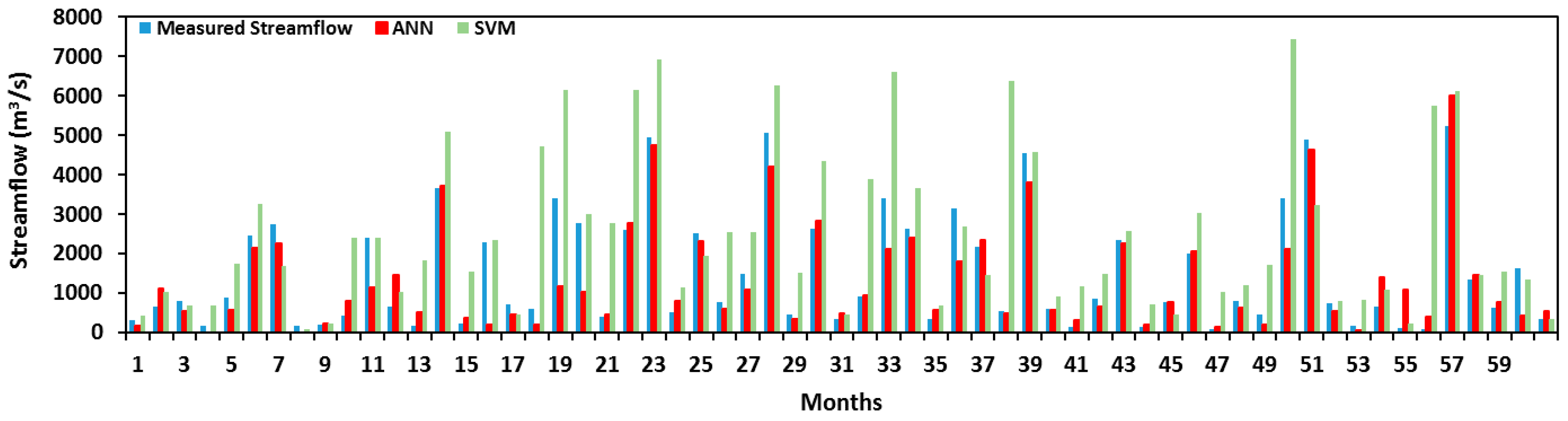
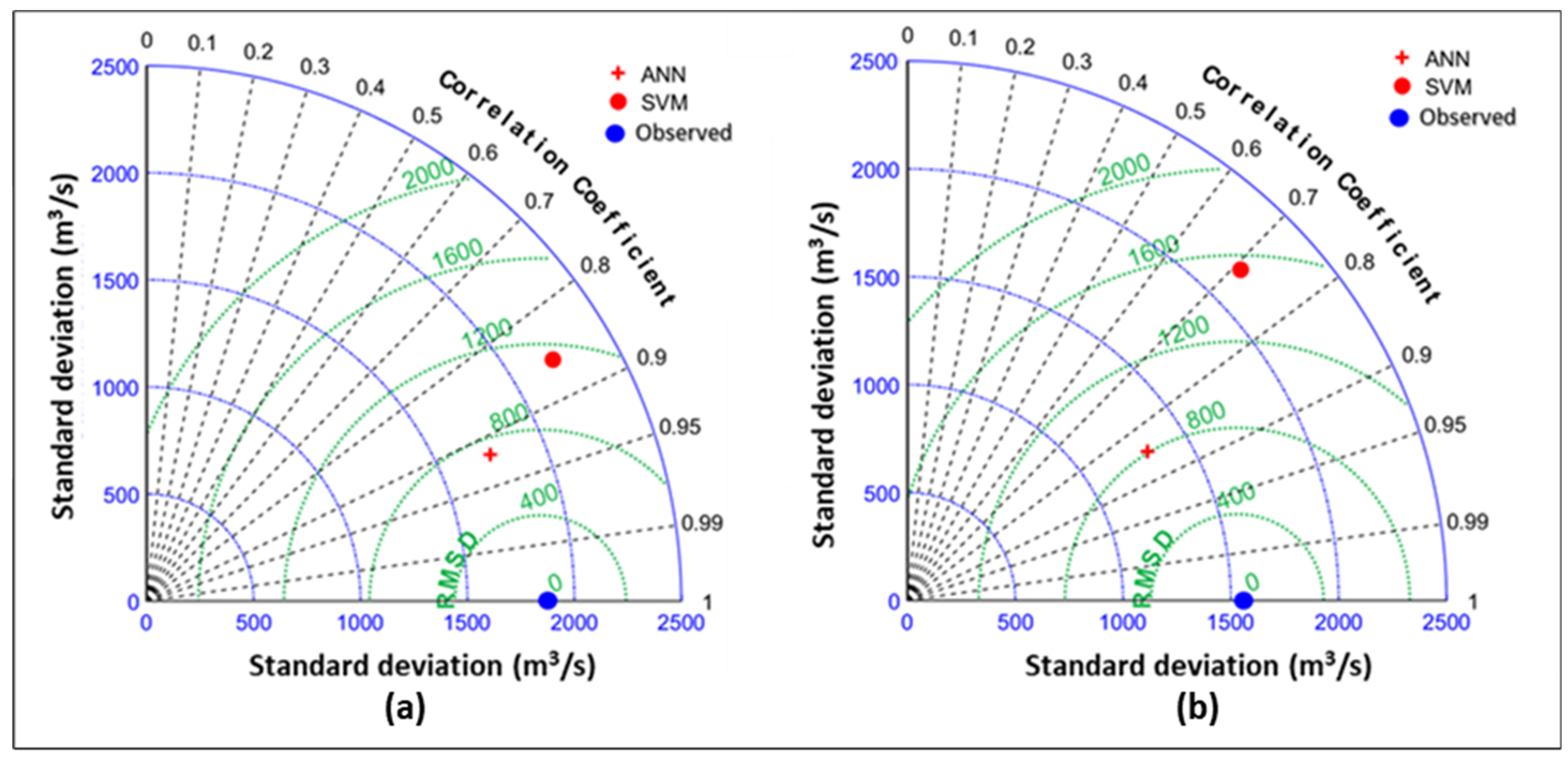
Table 3 presents the results of the model performance evaluation for the ANN and SVM models that confirm, in general, that the ANN performed better than the SVM. The overall comparison also revealed that the use of CHIRPS models for the forecasting streamflow is more appropriate than the use of models developed using the TRMM-3B42V7 and REF 2.0 datasets, which showed relatively low performance measures. To distinguish between the ANN and SVM models, the CHIRPS dataset of the last five years of the study period was used as input for the two models, and a comparison of the output of the ANN and SVM models, along with their corresponding measured streamflow, is presented in Figure 12. The findings shown in Figure 12 illustrate that the ANN model had superior performance than the CHIRPS-based SVM model. The additional statistical performance evaluation of the developed models was performed using the Taylor diagram (Figure 7), which describes the statistical patterns of developed models and their relative position from the measured streamflow in terms of their correlation, their root mean square difference, and the ratio of their variances [48]. Figure 13 confirms that the performance of the ANN model was the strongest and the most realistic in the training and testing periods since it was located closer to the reference line (RMSD) and the historical dataset.

4. Discussion

We compared three grid precipitation datasets of historical rainfall records and evaluated the hydrological performance of these datasets in forecasting streamflow. In a variety of previous studies, statistical assessments of the grided precipitation products were performed on small to large regions [33,34]. Furthermore, the hydrological evaluation of satellite products has also been investigated in several basins [27,28,29,35]. Musie [28] evaluated the capability of four satellite products to simulate streamflow in Ethiopia and reported that the performance of CHIRPS was the best. Likewise, in our analysis, the monthly Cr, ME, and BIAS values revealed that the three satellite-based products behaved differently, and CHIRPS performed better than the other two products. The RFE product overestimated rainfall quantities, which resulted in higher ME and BIAS values. This result demonstrates that while RFE was capable of identifying rainfall patterns, the rainfall quantities were significantly biased, which would result in streamflow with greater peak flow than measured. Regarding the proposed forecasting models, the ANN model performed much better than the SVM, which produced the highest R², the minimum RMSE, and the maximum E. The performance measures of the ANN model showed a relatively small drop from the training to testing phases; however, some of these measures obtained by the SVM were poor.

The SVM overestimated the monthly streamflow, as presented in Figure 12; however, the simulated values of streamflow using the ANN model were closer to the historical records. Additional distinct insights emerge in Figure 12 and Figure 13, which display the discrepancy between forecasted and historical streamflow records for the two models. The two figures show that the values obtained using SVM were significantly higher than the measured values, in which the SVM tended to overestimate streamflow records; however, the ANN model tended to underestimate streamflow for some individual months. The ANN using CHIRPS performed better than when using TRMM-3B42V7 and RFE 2.0 in the testing period. RFE 2.0 and TRMM-3B42V7 had greater statistical MAE and BIAS values than CHIRPS, which resulted in the relatively low performance in the testing phase results (Figure 11) and an overall overestimation of the streamflow. Based on our results, the high performance of the CHIRPS product indicates that this product could be used for streamflow forecasting with reasonable accuracy. It is worth mentioning that the training and testing of the ANN and SVM models were found to be sensitive to both the length of the satellite products dataset and the correlation between the gauge records and the satellite products dataset. The developed forecasting models using CHIRPS therefore performed much better than when using RFE 2.0 and TRMM-3B42V7 in this study. Consequently, it is highly recommended to evaluate other satellite products such as PERSIANN-CDR that have been shown to provide good performance in hydrologic applications [49,50,51,52,53,54,55] and cover a relatively long period (from 1983 to present) compared to RFE 2.0 and TRMM-3B42V7.

5. Conclusions

In the present study, we attempted to measure the statistical performance of three satellite-based precipitation products and compare their performance as input into ANN and SVM models for streamflow forecasting at El Diem station located along the upper Blue Nile River. In the training phase, a randomization procedure was implemented to evaluate the potential of inputs to create a more reliable and robust model in the development of ANN and SVM. Furthermore, the parameters of the two forecasting models were optimized to minimize the RMSE. The results of the precipitation product assessment confirmed that in both statistical and hydrological assessments, the CHIRPS product had the strongest performance. Furthermore, CHIRPS performed well as the input for the proposed forecasting models and provided a precise estimate of streamflow in the training and testing models. A comparison between the forecasted and historical streamflow records, using several evaluation criteria, confirmed the accuracy and effectiveness of the applied models and indicated that, in comparison to the SVM model, a relatively better resemblance of streamflow pattern was achieved by the ANN model, which can be recommended for streamflow forecasting. Finally, this work’s main conclusion is that combining ANN and SVM with satellite-based precipitation products could provide a highly useful tool for streamflow forecasting. Although the project of the Grand Ethiopian Renaissance Dam upstream of El Diem station will result in a decrease and irregularity in the inflow volume to this station over the coming years, the proposed ANN model showed satisfactory results and could be used as a simple tool for forecasting monthly streamflow upstream of this dam.

References

- Abrahart, R.J.; See, L. Comparing neural network and autoregressive moving average techniques for the provision of continuous river flow forecasts in two contrasting catchments. Hydrol. Process. 2000, 14, 2157–2172. [Google Scholar] [CrossRef]
- Wu, C.; Chau, K.; Li, Y. Predicting monthly streamflow using data-driven models coupled with data-preprocessing techniques. Water Resour. Res. 2009, 45, 1–23. [Google Scholar] [CrossRef] [Green Version]
- Valipour, M. Long-term runoff study using SARIMA and ARIMA models in the United States. Meteorol. Appl. 2015, 22, 592–598. [Google Scholar] [CrossRef]
- Srivastava, P.K.; Han, D.; Ramirez, M.R.; Islam, T. Machine Learning Techniques for Downscaling SMOS Satellite Soil Moisture Using MODIS Land Surface Temperature for Hydrological Application. Water Resour. Manag. 2013, 27, 3127–3144. [Google Scholar] [CrossRef]
- Adams, T.E., III; Chen, S.; Dymond, R. Results from operational hydrologic forecasts using the NOAA/NWS OHRFC Ohio river community HEC-RAS model. J. Hydrol. Eng. 2018, 23, 04018028. [Google Scholar] [CrossRef]
- Bagatur, T.; Onen, F. Development of predictive model for flood routing using genetic expression programming. J. Flood Risk Manag. 2018, 11, S444–S454. [Google Scholar] [CrossRef] [Green Version]
- Yaseen, Z.M.; Jaafar, O.; Deo, R.C.; Kisi, O.; Adamowski, J.; Quilty, J.; El-Shafie, A. Stream-flow forecasting using extreme learning machines: A case study in a semi-arid region in Iraq. J. Hydrol. 2016, 542, 603–614. [Google Scholar] [CrossRef]
- Kasiviswanathan, K.; He, J.; Sudheer, K.; Tay, J.-H. Potential application of wavelet neural network ensemble to forecast streamflow for flood management. J. Hydrol. 2016, 536, 161–173. [Google Scholar] [CrossRef]
- Muhammad, S.; Asaad, Y.; Shamseldin, B.; Melville, W.; Mudasser, M.K. Hybrid Wavelet Neural Network Approach. In Artificial Neural Network Modelling; Springer: Berlin, Germany, 2016; pp. 127–143. [Google Scholar]
- Bertone, E.; O’Halloran, K.; Stewart, R.A.; de Oliveira, G.F. Medium-term storage volume prediction for optimum reservoir management: A hybrid data-driven approach. J. Clean. Prod. 2017, 154, 353–365. [Google Scholar] [CrossRef] [Green Version]
- Dariane, A.; Farhani, M.; Azimi, S. Long term streamflow forecasting using a hybrid entropy model. Water Resour. Manag. 2018, 32, 1439–1451. [Google Scholar] [CrossRef]
- Allawi, M.F.; Jaafar, O.; Hamzah, F.M.; Abdullah, S.M.S.; El-Shafie, A. Review on applications of artificial intelligence methods for dam and reservoir-hydro-environment models. Environ. Sci. Pollut. Res. 2018, 25, 13446–13469. [Google Scholar] [CrossRef] [PubMed]
- Modini, G.C. Long-lead precipitation outlook augmentation of multi-variate linear regression streamflow forecasts. In Proceedings of the 68th Annual Western Snow Conference, Port Angeles, WA, USA, 17–20 April 2000. [Google Scholar]
- Khan, M.Y.A.; Hasan, F.; Panwar, S.; Chakrapani, G.J. Neural network model for discharge and water-level prediction for Ramganga River catchment of Ganga Basin, India. Hydrol. Sci. J. 2016, 61, 2084–2095. [Google Scholar] [CrossRef] [Green Version]
- Khan, M.Y.A.; Hasan, F.; Panwar, S.; Chakrapani, G.J. Typhoon event-based evolutionary fuzzy inference model for flood stage forecasting. J. Hydrol. 2013, 490, 134–143. [Google Scholar]
- Ch, S.; Anand, N.; Panigrahi, B.K.; Mathur, S. Streamflow forecasting by SVM with quantum behaved particle swarm optimization. Neurocomputing 2013, 101, 18–23. [Google Scholar] [CrossRef]
- Feng, C.; Cui, M.; Hodge, B.-M.; Zhang, J. A data-driven multi-model methodology with deep feature selection for short-term wind forecasting. Appl. Energy 2017, 190, 1245–1257. [Google Scholar] [CrossRef] [Green Version]
- Liu, Z.; Zhou, P.; Chen, G.; Guo, L. Evaluating a coupled discrete wavelet transform and support vector regression for daily and monthly streamflow forecasting. J. Hydrol. 2014, 519, 2822–2831. [Google Scholar] [CrossRef]
- Mohammadpour, R.; Shaharuddin, S.; Chang, C.K.; Zakaria, N.A.; Ab Ghani, A.; Chan, N.W. Prediction of water quality index in constructed wetlands using support vector machine. Environ. Sci. Pollut. Res. 2014, 22, 6208–6219. [Google Scholar] [CrossRef]
- Poul, A.K.; Shourian, M.; Ebrahimi, H. A comparative study of MLR, KNN, ANN and ANFIS models with wavelet transform in monthly stream flow prediction. Water Resour. Manag. 2019, 33, 2907–2923. [Google Scholar] [CrossRef]
- Gong, Y.; Zhang, Y.; Lan, S.; Wang, H. A Comparative Study of Artificial Neural Networks, Support Vector Machines and Adaptive Neuro Fuzzy Inference System for Forecasting Groundwater Levels near Lake Okeechobee, Florida. Water Resour. Manag. 2016, 30, 375–391. [Google Scholar] [CrossRef]
- Hosseini, S.M.; Mahjouri, N. Integrating support vector regression and a geomorphologic artificial neural network for daily rainfall-runoff modeling. Appl. Soft Comput. 2016, 38, 329–345. [Google Scholar] [CrossRef]
- Dehghani, N.; Vafakhah, M.; Bahremand, A. Rainfall-runoff modeling using artificial neural network and neuro-fuzzy inference system in kasilian watershed. J. Watershed Manag. Res. 2016, 7, 128–137. [Google Scholar]
- Zare, M.; Koch, M. Using ANN and ANFIS Models for simulating and predicting groundwater level fluctuations in the Miandarband Plain, Iran. In Proceedings of the 4th IAHR Europe Congress. Sustainable Hydraulics in the Era of Global Change, Liege, Belgium, 27 July 2016; p. 416. [Google Scholar]
- Vetrivel, N.; Elangovan, K. Application of ANN and ANFIS model on monthly groundwater level fluctuation in lower Bhavani River Basin. Indian J. Geo. Mar. Sci. 2017, 46, 2114–2121. [Google Scholar]
- Tabbussum, R.; Dar, A.Q. Performance evaluation of artificial intelligence paradigms—Artificial neural networks, fuzzy logic, and adaptive neuro-fuzzy inference system for flood prediction. Environ. Sci. Pollut. Res. 2021, 28, 1–18. [Google Scholar] [CrossRef]
- Javanmard, S.; Yatagai, A.; Nodzu, M.I.; BodaghJamali, J.; Kawamoto, H. Comparing high-resolution gridded precipitation data with satellite rainfall estimates of TRMM_3B42 over Iran. Adv. Geosci. 2010, 25, 119–125. [Google Scholar] [CrossRef] [Green Version]
- Musie, M.; Sen, S.; Srivastava, P. Comparison and evaluation of gridded precipitation datasets for streamflow simulation in data scarce watersheds of Ethiopia. J. Hydrol. 2019, 579, 124168. [Google Scholar] [CrossRef]
- Beven, K.; Westerberg, I. On red herrings and real herrings: Disinformation and information in hydrological inference. Hydrol. Process. 2011, 25, 1676–1680. [Google Scholar] [CrossRef]
- Nguyen-Xuan, T.; Ngo-Duc, T.; Kamimera, H.; Trinh-Tuan, L.; Matsumoto, J.; Inoue, T.; Phan-Van, T. The Vietnam Gridded Precipitation (VnGP) Dataset: Construction and Validation. SOLA 2016, 12, 291–296. [Google Scholar] [CrossRef] [Green Version]
- Tapiador, F.J.; Turk, F.J.; Petersen, W.; Hou, A.Y.; García-Ortega, E.; Machado, L.A.; Carlos, F.; Angelis, P.S.; Chris, K.; George, J.; et al. Global precipitation measurement: Methods, datasets and applications. Atmos. Res. 2012, 104, 70–97. [Google Scholar] [CrossRef]
- Nijssen, B.; Lettenmaier, D.P. Effect of precipitation sampling error on simulated hydrological fluxes and states: Anticipating the Global Precipitation Measurement satellites. J. Geophys. Res. Atmos. 2004, 109, 1–15. [Google Scholar] [CrossRef]
- Abd Elhamid, A.M.; Eltahan, A.M.; Mohamed, L.M.; Hamouda, I.A. Assessment of the two satellite-based precipitation products TRMM and RFE rainfall records using ground based measurements. Alex. Eng. J. 2020, 59, 1049–1058. [Google Scholar] [CrossRef]
- Sulugodu, B.; Deka, P.C. Evaluating the performance of CHIRPS satellite rainfall data for streamflow forecasting. Water Resour. Manag. 2019, 33, 3913–3927. [Google Scholar] [CrossRef]
- Nguyen, P.; Ombadi, M.; Sorooshian, S.; Hsu, K.; AghaKouchak, A.; Braithwaite, D.; Ashouri, H.; Thorstensen, A.R. The PERSIANN family of global satellite precipitation data: A review and evaluation of products. Hydrol. Earth Syst. Sci. 2018, 22, 5801–5816. [Google Scholar] [CrossRef] [Green Version]
- Huffman, G.J.; Bolvin, D.T.; Nelkin, E.J. Integrated Multi-satellitE Retrievals for GPM (IMERG) technical documentation. NASA/GSFC Code 2015, 612, 2019. [Google Scholar]
- Maidment, R.I.; Grimes, D.; Allan, R.P.; Tarnavsky, E.; Stringer, M.; Hewison, T.; Roebeling, R.; Black, E. The 30 year TAMSAT African Rainfall Climatology And Time series (TARCAT) data set. J. Geophys. Res. Atmos. 2014, 119, 10619–10644. [Google Scholar] [CrossRef] [Green Version]
- Tarnavsky, E.; Grimes, D.; Maidment, R.; Black, E.; Allan, R.; Stringer, M.; Chadwick, R.; Kayitakire, F. Extension of the TAMSAT Satellite-Based Rainfall Monitoring over Africa and from 1983 to Present. J. Appl. Meteorol. Clim. 2014, 53, 2805–2822. [Google Scholar] [CrossRef] [Green Version]
- Conway, D. The climate and hydrology of the Upper Blue Nile River. Geogr. J. 2000, 166, 49–62. [Google Scholar] [CrossRef] [Green Version]
- Nour-El-Din, M.M. Climate Change Risk Management in Egyp: Proposed Climate Change Adaptation Strategy for the Ministry of Water Resources & Irrigation in Egypt. 2013. Available online: https://research.fit.edu/media/site-specific/researchfitedu/coast-climate-adaptation-library/africa/egypt-amp-libya/EL-Din.--2013.--Ministry-of-Water-Resource--Irrigation.pdf (accessed on 11 October 2021).
- Funk, C.C.; Peterson, P.J.; Landsfeld, M.F.; Pedreros, D.H.; Verdin, J.P.; Rowland, J.D.; Romero, B.E.; Husak, G.J.; Michaelsen, J.C.; Verdin, A.P. A quasi-global precipitation time series for drought monitoring. US Geol. Surv. Data Ser. 2014, 832, 1–12. [Google Scholar]
- Chen, C.; Chen, Q.; Duan, Z.; Zhang, J.; Mo, K.; Li, Z.; Tang, G. Multiscale Comparative Evaluation of the GPM IMERG v5 and TRMM 3B42 v7 Precipitation Products from 2015 to 2017 over a Climate Transition Area of China. Remote Sens. 2018, 10, 944. [Google Scholar] [CrossRef] [Green Version]
- Kim, K.; Park, J.; Baik, J.; Choi, M. Evaluation of topographical and seasonal feature using GPM IMERG and TRMM 3B42 over Far-East Asia. Atmos. Res. 2017, 187, 95–105. [Google Scholar] [CrossRef]
- Kecman, V. Learning and Soft Computing: Support Vector Machines, Neural Networks, and Fuzzy Logic Models; MIT Press: Cambridge, MA, USA, 2001. [Google Scholar]
- Lafdani, E.K.; Nia, A.M.; Ahmadi, A. Daily suspended sediment load prediction using artificial neural networks and support vector machines. J. Hydrol. 2013, 478, 50–62. [Google Scholar] [CrossRef]
- Bafitlhile, T.M.; Li, Z. Applicability of ε-support vector machine and artificial neural network for flood forecasting in humid, Semi-Humid and Semi-Arid Basins in China. Water 2019, 11, 85. [Google Scholar] [CrossRef] [Green Version]
- Nash, J.E.; Sutcliffe, J.V. River flow forecasting through conceptual models part I—A discussion of principles. J. Hydrol. 1970, 10, 282–290. [Google Scholar] [CrossRef]
- Taylor, K.E. Summarizing multiple aspects of model performance in a single diagram. J. Geophys. Res. Atmos. 2001, 106, 7183–7192. [Google Scholar] [CrossRef]
- Santos, C.A.G.; Neto, R.M.B.; Nascimento, T.V.M.D.; da Silva, R.M.; Mishra, M.; Frade, T.G. Geospatial drought severity analysis based on PERSIANN-CDR-estimated rainfall data for Odisha state in India (1983–2018). Sci. Total. Environ. 2021, 750, 141258. [Google Scholar] [CrossRef] [PubMed]
- Arvor, D.; Funatsu, B.M.; Michot, V.; Dubreuil, V. Monitoring Rainfall Patterns in the Southern Amazon with PERSIANN-CDR Data: Long-Term Characteristics and Trends. Remote Sens. 2017, 9, 889. [Google Scholar] [CrossRef] [Green Version]
- Bâ, K.M.; Balcázar, L.; Diaz, V.; Ortiz, F.; Gómez-Albores, M.A.; Díaz-Delgado, C. Hydrological Evaluation of PERSIANN-CDR Rainfall over Upper Senegal River and Bani River Basins. Remote Sens. 2018, 10, 1884. [Google Scholar] [CrossRef] [Green Version]
- Mosaffa, H.; Sadeghi, M.; Hayatbini, N.; Afzali Gorooh, V.; Akbari Asanjan, A.; Nguyen, P.; Sorooshian, S. Spatiotemporal variations of precipitation over Iran using the high-resolution and nearly four decades satellite-based PERSIANN-CDR dataset. Remote Sens. 2020, 12, 1584. [Google Scholar] [CrossRef]
- Ombadi, M.; Nguyen, P.; Sorooshian, S.; Hsu, K. Developing Intensity-Duration-Frequency (IDF) Curves From Satellite-Based Precipitation: Methodology and Evaluation. Water Resour. Res. 2018, 54, 7752–7766. [Google Scholar] [CrossRef]
- Ombadi, M.; Nguyen, P.; Sorooshian, S.; Hsu, K.-L. Retrospective Analysis and Bayesian Model Averaging of CMIP6 Precipitation in the Nile River Basin. J. Hydrometeorol. 2021, 22, 217–229. [Google Scholar] [CrossRef]
- Ashouri, H.; Nguyen, P.; Thorstensen, A.; Hsu, K.-L.; Sorooshian, S.; Braithwaite, D. Assessing the Efficacy of High-Resolution Satellite-Based PERSIANN-CDR Precipitation Product in Simulating Streamflow. J. Hydrometeorol. 2016, 17, 2061–2076. [Google Scholar] [CrossRef]
Figure 1.
Location map of the study area showing the digital elevation model (DEM) of the upper Blue Nile River basin and the selected meteorological stations.
Figure 2.
Methodological framework to forecast monthly streamflow.
Figure 3.
Arrangement of the ANN used in this study.
Figure 4.
Box plots of monthly rainfall distributions for the satellite products and gauge records at the Abasina Joger and Arjo stations: TRMM-3B42V7 from 1998 to 2014, CHIRPS from 1981 to 2014, and RFE from 1983 to 2014.
Figure 5.
Box plots of monthly rainfall distributions for the satellite products and gauge records at the Bahir Dar and Combolocha stations: TRMM-3B42V7 from 1998 to 2014, CHIRPS from 1981 to 2014, and RFE from 1983 to 2014.
Figure 6.
Scatter plots of the satellite products and gauge records.
Figure 7.
Correlation between observed rain gauge and river flow at El Diem station at lag 0, lag 1, and lag 2 at a monthly scale (1966–2008).
Figure 8.
SVM training and test results of the simulated monthly streamflow at El Diem station based on the CHIRPS dataset.
Figure 9.
ANN training and test results of the simulated monthly streamflow at El Diem station based on the CHIRPS dataset.
Figure 10.
ANN test results of the simulated monthly streamflow at El Diem station based on TRMM-3B42V7 and RFE 2.0 data.
Figure 11.
SVM test results of the simulated monthly streamflow at El Diem station based on TRMM-3B42V7 and RFE 2.0 data.
Figure 12.
Comparison of streamflow forecasting results using the ANN and SVM models with the measured streamflow for the last five years of the testing period based on CHIRPS data.
Figure 13.
Taylor diagram for the ANN and SVM compared to the observed data: (a) training; (b) testing.