1. Introduction
With the emergence of the concepts of the “smart city” and “twin city”, and the continued advancement of related research, how to carry out rapid data collection and environmental perception of urban scenes is becoming a research hotspot. The road scene is one of the most important components of the urban environment. Both sides of the road contain rich feature information, such as buildings, rods, and low vegetation. Pole-like objects are important subsidiary components of the road scene and can reflect changes in road characteristics in real time. How to realize the rapid recognition of pole-like objects has great significance to the ubiquitous perception of the urban scene and the census of road resources [
1,
2,
3].
Compared with traditional methods, mobile lidar is a newer type of road environment information collection method that can quickly and efficiently obtain real-time access to roads and its auxiliary facilities as well as partial building facades. It can also realize the synchronous acquisition of image data and point cloud data, and enormously enrich the content of data acquisition. Moreover, the obtained data are more detailed, providing a solid basic foundation for road scene environment perception [
4,
5,
6].
At present, pole-like object extraction and classification methods based on the point clouds of road scenes can be divided into three main categories: the method based on the structural features of the pole-like objects [
7,
8,
9], the method based on clustering before recognition [
10,
11,
12], and the method based on template matching [
13,
14]. Li et al. [
15] first horizontally projected the original point clouds in a road scene, then formed a single grid as a processing unit for ground point removal. Considering the height difference, shape, and projection of the pole-like object point clouds and using the clustering method to extract pole-like objects without considering the situation of overlapping pole-like objects, the universality and robustness of this method are not high enough. Kang et al. [
16] used an adaptive voxel method to extract the pole-like objects according to their geometric shape, and then completed the recognition of the pole-like objects by combining the shape and spatial topological relationship, which showed a good recognition effect on the three experimental datasets. However, this method has a strong dependence on the results of voxel extraction owing to the disadvantages of the method, so this method cannot complete and correct extraction for large pole-like objects. Huang et al. [
17] proposed a fusion divergence clustering algorithm, which first extracts the rod-shaped parts of the pole-like objects and then combines them with the adaptive growth strategy of alternating expansion and renewal of the 3D neighborhood to obtain complete canopy points with different shapes and densities. Combined with the parameterization method to classify the pole-like objects, the robustness of this method for overlapping scenes is poor.
Thanh et al. [
18] extracted the road rod-shaped facilities by using the horizontal section analysis and minimum vertical height criterion, and then constructed a set of knowledge rules, including height features and geometric features to divide the road pole-like objects into different types. However, this method is not robust for the extraction of pole-like objects with a large inclination. Liu et al. [
19] proposed a hierarchical classification method to extract the pole-like objects, and then identified the extracted pole-like objects in combination with an eigenvalue analysis and principal direction. However, this method is not ideal when the point density is sparse, and the noise is widespread. Andrade et al. [
20] proposed a three-step method to extract and classify pole-like objects. First, the variance and covariance matrix of the segmentation objects is calculated, the eigenvalue and eigenmatrix are derived to carry out the 3D coordinate transformation of the point cloud objects, and the new feature calculation is carried out in the new transformation space. Second, the feature values distributed in the feature space are analyzed, and afterward, the classification method based on line distance is used to classify the vertical features. The disadvantage of this method is that the eigenvalues are highly sensitive to point clouds, which means this method has high requirements for the noise and density of point clouds. When the data effect is not good enough, the classification effect obtained is not ideal. Li et al. [
21] proposed a dense-based 3D segmentation algorithm, which considers the overlapping and non-overlapping pole-like objects and uses a new shape distribution estimation method to obtain a more robust global descriptor. The integrated shape constraint based on the segmentation results of pole-like objects is used for object classification and integrated into the retrieval process. In the test, the data showed a good effect. Tang et al. [
22] used the combination of Euclidean clustering and the minimum cut method to segment the point cloud of the road scene based on the entity unit, and finally completed the semantic classification of pole-like traffic facilities of the road scene with the SVM classifier. The algorithm has low accuracy for small targets and incomplete pole-like objects.
Zhang et al. [
23] first extracted the sample parameters of street lamps through human-computer interaction, and then extracted the point clouds suspected to be street lamps in the road scene according to the mathematical morphology operation. On this basis, a match was made between the two to complete the type recognition of street lamps. This method has strong robustness in segmentation results, and has a good processing effect for some special entities, such as entities containing multiple affiliated facilities or entities with multiple overlapping targets. However, this method requires high robustness for local feature descriptors. Yu et al. [
24] completed template matching among objects based on pre-divided point cloud scenes. This method requires a substantial prior template, cannot match entities that do not exist in the template, and has low matching efficiency.
The above reviews show that in the identification of pole-like objects in the road scenes, the method based on structural features is not efficient in identifying pole-like objects that have similar features, and is susceptible to noise interference. The method of clustering before recognition has a high requirement on the integrity of the segmentation results, which often shows unsatisfactory performance in some overlapping or occlusion scenes, and only the local features or global features of point clouds are taken into account in the process of recognition. However, the mutual assistance between features is not taken into account. The method based on template matching requires a lot of human-computer interaction and shows a low degree of automation and low computational efficiency.
In this paper, the recognition of pole-like objects is divided into two stages: segmentation and classification. In the first stage, the geometric features of the pole-like objects are used to complete the extraction of pole-like objects. Then, in the second stage, we improve the recognition accuracy of pole-like objects by combining the recognition results at different scales. Our contributions are as follows:
By extracting pole-like objects using the geometric features of the rods, the details of the pole-like objects are retained by the voxel growth and one-way double coding strategy. The integrity of pole-like objects extraction is significantly enhanced;
The pole-like objects are recognized based on the features at different scales, and the results are merged so that the recognition results at different scales can complement each other and effectively improve the accuracy of recognition.
The rest of this article is organized as follows.
Section 2 describes the specific approach proposed.
Section 3 shows and analyzes the experiment results.
Section 4 provides a discussion and analysis of the results.
Section 5 summarizes this article and details future work.
2. Materials and Methods
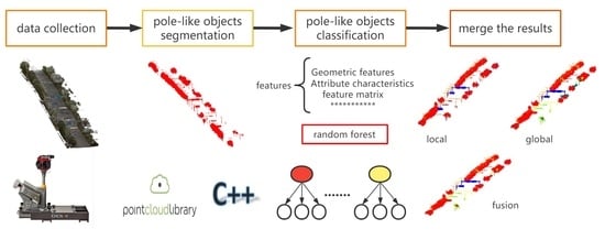
The vehicle-mounted lidar is a passive way of mobile scanning that can quickly and accurately obtain information on both sides of roads. However, owing to the different distances between the scanning target and the laser emission center, the different scanning viewpoints, and the mutual occlusion between the targets, the target point cloud density is different and point clouds may be missing, which brings challenges to the classification of the target point cloud. Therefore, this paper proposes a strategy that combines voxel segmentation and voxel growth to extract pole-like objects. Then, we used the method of fusion of local feature and global feature classification results to identify different pole-like objects. The experimental results indicated that the method can quickly extract and accurately identify the pole-like objects of the road scene point clouds. The technical route of the method is shown in
Figure 1 below.
2.1. Experimental Data
The Alpha3D vehicle-mounted mobile measurement system was used to collect the data of an urban road. The horizontal accuracy of the system is <0.030 m RMS, and the vertical accuracy is <0.025 m RMS. The laser point frequency of the system can reach 1,000,000 points/s, the measurement accuracy can reach 5 mm, and the repeated measurement accuracy can reach 2 mm. The point cloud data of the road scene obtained are shown in
Figure 2. A total of 1-km long street view experimental data were collected, with a size total of 1.5 GB and 60,244,135 points, including natural pole-like objects, artificial pole-like objects, vehicles, and low vegetation.
2.2. Extraction of Pole-Like Objects
The common pole-like objects in urban road scenes can be divided into artificial pole-like objects and natural pole-like objects. The main bodies of the pole-like objects have the characteristics of vertical continuity in geometric composition, and the non-rod-shaped parts of the pole-like objects generally extend vertically to the main part of the rod-shaped parts in space. The pole-like objects of the same class are similar in geometric structure, but the pole-like objects of different classes generally have differences in height, radius, and non-rod-shaped parts. The differences between non-rod-shaped parts in the vehicular laser scanning data are mainly manifested in intensity, curvature, transverse extension distance, and local and global morphological composition. Here, low-rise vegetation was not used as pole-like objects to study.
Based on the above analysis, this method processes the point clouds into voxels first, according to the characteristics of the pole-like objects with vertical continuity to extract the rod-shaped parts. For the extracted non-rod-shaped parts, we adopt a kind of lateral growth strategy based on the voxels to reserve the non-rod-shaped parts. As for compositions that do not directly connect with rod-shaped parts, we adopt a one-way double coding strategy to retain the details of the non-rod-shaped parts. Finally, the extracted parts are cleaned based on height difference and density to derive the cleaning pole-like road facilities from the mobile laser scanning data.
2.2.1. Data Preprocessing
The preprocessing stage mainly includes two processes: ground point filtering and point cloud downsampling. Filtering and downsampling of the original point clouds can reduce the amount of subsequent calculation and reduce the interference of some non-pole-like objects in the process of the pole-like object extraction. Ground point filtering is where a large number of ground point clouds are included in the acquisition process of vehicle-mounted lidar data, and these ground point clouds cause non-negligible interference to the subsequent extraction of pole-like objects. Combined with the characteristics of good continuity and small slope fluctuations in the point clouds of road scenes, the cloth simulation filter (CSF) [
25] is used to filter the ground points of the original point clouds. In terms of downsampling, the uniform downsampling method is used to downsample the original point clouds.
2.2.2. The Process of Pole-Like Object Segmentation
The pre-processed point clouds are voxelized based on the global coordinate, and the continuous voxels in the vertical direction are retained according to the vertical continuity of the pole-like objects. The point clouds in the voxels are the rod-shaped parts of the pole-like objects, and the non-rod parts are retained based on the rod-shaped parts. The overall process is as follows:
The maximum and minimum coordinates of the point clouds in the point cloud data are found after preprocessing, and then the maximum and minimum coordinates in the x-direction, y-direction, and z-direction are used as constraints to establish 3D voxels with a fixed length of S, each voxel has a vertical height,
H. We used each vertical column as the basic unit to encode the voxel from bottom to top. In the encoding process, the voxel with a point cloud is marked as 1, and the voxel without a point cloud is marked as 0. The calculations of 3D voxels are formulated as:
where
,
, and
represent the number of voxels in the X-axis, Y-axis, and Z-axis directions, respectively.
,
,
,
,
, and
represent the maximum and minimum coordinate values of the pre-processed point clouds. The representation of the position of one point cloud in a voxel is formulated as:
where
M, N, and
H represent the row coding, column coding, and vertical coding of point cloud in the voxel, respectively. Moreover, point.x, point.y, and point.z represent the specific coordinate value of one point after pre-processing.
- 2.
Retention of Vertical Voxels:
When the continuous 3D voxels appear in a vertical column and have point clouds that fall into the 3D voxel, these voxels will be retained, and the retained point clouds are the rod-shaped part of the pole-like objects. The schematic diagram of the retention method is shown in
Figure 3.
- 3.
Regional growth based on voxels and the one-way double coding strategy:
After the rod parts of pole-like objects are retained according to the vertical continuity above, only the rod-shaped parts on both sides of the road are obtained, but the non-rod-shaped parts of pole-like objects are not obtained. In order to reduce the calculation amount and retain the non-rod-shaped parts, horizontal regional growth based on the voxel algorithm is adopted. The main idea of this algorithm is to use the voxels that retain the rod-shaped parts as the reference to set up a local space coordinate system, and then divide the local space into four quadrants. Based on the above-mentioned voxels that diverge the query in the 3D space, and according to the condition that the non-rod-shaped part is horizontally connected to the rod-shaped part in the morphological structure, if there is a continuously diverging horizontal voxel around the reference voxel, it is considered to be the non-rod-shaped part of the pole-like objects and to reserve non-rod-shaped point clouds. The coordinate system established is shown in
Figure 4.
After completing the above steps, the non-rod parts of the pole-like objects are still omitted, especially objects that are not connected to the rod-shaped parts of the pole-like objects directly, such as the second half of the traffic lights and the top half of traffic signs. Therefore, we adopt a one-way double coding strategy for secondary reservation. The mathematical model of the one-way double coding method is expressed as: D (n1, n2), where n1 represents the bottom-up voxel coding number, and n2 represents the bottom-up voxel coding number where the point clouds exist.
Figure 5 shows the coding method.
The idea central to this method is that the voxel of each vertical column is taken as the research object, and one of the double codes encodes from the lowest voxel to the highest. In the other coding process, the voxel in which the point clouds appear is used as the initial voxel, and while the voxel contains point clouds, it will be encoded continuously. The above-mentioned unretained point cloud data are retained by using the feature of the difference between the double codes, as the difference in the details of the pole-like objects is obvious. Meanwhile, for low-rise vegetation, the two codes are close to each other, so low-rise vegetation can also be filtered out. The pole-like object point clouds after these two steps are shown in
Figure 6.
2.2.3. Pole-Like Object Cleaning
Figure 6 shows that there are still some noise points among the extracted pole-like objects, which are caused by the improper scale of the voxel and unsatisfactory detail expression. Therefore, the retained pole-like objects tend to be retained together when the surrounding objects are adhered to. Another major reason is that the height of some low vegetation is high, and the low-rise vegetation is also retained as rod-shaped parts in the vertical continuity search.
In order to obtain cleaning pole-like objects point cloud data, we use Euclidean distance clustering [
26] and the height of the projection method to clean the pole-like object point clouds. First, point clouds with similar distances are divided into the same point cloud cluster through Euclidean metric clustering. When the number of point clusters is too small, the point clouds are considered to be the noise point clouds and are filtered out in units of clusters. Euclidean distance clustering can effectively remove some outliers. After the outliers are removed, the point clouds are projected on the Z-axis, and the projected point clouds are divided into smaller voxels than those mentioned in the above. When the height difference and the maximum z-value are less than the threshold value, these point clouds that are contained in the voxels are dropped because they are low-vegetation point clouds.
Through the above two steps, the obtained pole-like objects point cloud data can be cleaned, and the influence of non-rod-shaped point clouds on the pole-like object classification can be effectively reduced. The clean point cloud data are shown in
Figure 7.
2.3. Fusion of Multiscale Pole-Like Object Recognition
Based on the segmentation of the pole-like object point clouds, the classification and attribute acquisition are carried out. Traditional machine learning classification methods do not consider comprehensive features, and the scale is relatively simple. In view of this shortcoming, this paper adopts the method of the fusion of local feature classification results and global feature classification results, and combines the two categories of labels to determine the final classification results.
2.3.1. Pole-Like Object Classification Based on the Local Feature
In the local feature recognition of point clouds, each point cloud is first taken as the research object to establish local feature space, and then the feature space of each point cloud is taken as the computing unit to calculate the feature of the point clouds. The 14-dimensional features are defined to describe the difference of the pole-like objects on both sides of the road, which can be generally summarized into four categories: height features, eigenvalue combination features, attribute features, and surface features.
Hight features: Height features include the height difference of point clouds and the variance within the sphere’s neighborhood. Moreover, a cylindrical region with a sphere neighborhood as the radius is divided, and the height difference within the cylindrical region is calculated. Such features can be used to exclude pole-like objects with large elevation differences. Examples include low sign boards and trees as well as street lights.
Attribute features: There are four types of attribute features, including intensity features, density features, volume density features, and the number of points in the cylindrical neighborhood. According to different pole-like object point clouds, densities are different to define the density feature. The definition of density is the number of a local sphere space‘s point clouds, and the point clouds number as the density descriptor can divide some differences in the density of pole-like objects [
27]. Different pole-like objects also have different echo intensities because of their different materials. For the surface structure, the smoother the surface, the greater the value of the intensity of the object point clouds; for the pole-like objects on both sides of the road, the reflection intensity of the sign is often greater than that of the other types of objects. We can use this information to distinguish some pole-like objects and increase the efficiency and accuracy of identification. Owing to the complexity of the structure of the road scene, different pole-like objects often show different density values within the same neighborhood, so we define the density feature as a property to distinguish different pole-like objects. The definition of the number of points in the cylindrical neighborhood is based on the pre-defined cylindrical neighborhood. Moreover, in the cylindrical neighborhood, we want to find the number of points contained because the structure of the pole-like object is vertical, and different pole-like objects contain different point cloud numbers in the same cylindrical neighborhood. Usually, tall pole-like objects contain more points, and low pole-like objects contain fewer points. Based on this characteristic, we define this feature as a property to identify the pole-like objects.
Eigenvalue combination features: These features include five categories, including local neighborhood anisotropy, plane features, spherical features, full variance features, and line features. According to [
28,
29,
30], we can calculate the covariance matrix and eigenvalue eigenvector in the sphere neighborhood and distinguish different entities by using the features composed by the combination of eigenvalues. The principle mainly applied is that the geometric composition of point clouds in the local neighborhood is different, and the geometric composition of point clouds can be represented by the combination of eigenvalues. For example, in trees, the point clouds of tree trunks show strong linear features and weak spherical features. The opposite is true in the geometric representation of the crown. The calculation equation is formulated as:
where
,
,
,
, and
represent the total variance, linear features, plane features, spherical features, and total variance of point cloud in the neighborhood space.
,
, and
are the eigenvalues calculated by the matrix in the neighborhood space of the point cloud, and the value of the three eigenvalues are decreasing.
Surface features: There are two types of surface features, including roughness and curvature. Curvature is a measure of the degree of curvature of a curve. In point clouds, curvature is divided into main curvature, mean curvature, and Gaussian curvature. Gaussian curvature is the quantity describing the concave-convex degree of a surface. When this quantity changes greatly, the internal change in the surface is also relatively large, which indicates that the smoothness of the surface is lower. The curvature of a point cloud can be expressed by the curvature of the local surface fitted by the point cloud and its neighborhood point clouds. The curvature type used in this paper is the Gaussian curvature calculation method. The calculation equation is formulated as:
where
E, F, and
G are the first basic invariants of the surface.
L, M, and
N are the second basic invariants of the surface. Roughness is the ratio of surface area to projected area in a certain area, which can be used to distinguish the signage parts and the non-signage parts in the pole-like object recognition process.
- 2.
Establishment of feature vectors:
According to the above-mentioned characteristics, based on the local neighborhood of the point clouds, we set up 14 dimensions of feature vectors and covered many aspects, such as intensity, elevation difference, elevation variance, anisotropy, plane features, sphere features, total variance, line features, point numbers of cylindrical what, elevation difference of cylindrical what, density, volume density, curvature, and roughness. Part of the pole-like objects were randomly selected as the training data, including seven types of signs: low signs, street lights, monitoring, trees, traffic lights, and low traffic lights. The established feature vectors are shown in
Table 1.
- 3.
Establishment of classifier model:
After defining the features, how to select the appropriate classifier is also an indispensable part of the classification process based on local features. Common classifiers include the neural network [
31], support vector machine [
32], and random forest [
33,
34]. Compared with other algorithms, random forest has its unique advantages, which mainly includes that it does not need to perform feature selection, it is more stable for processing high-dimensional data, and the calculation speed is fast. Therefore, the random forest model was selected as the training model in this paper.
2.3.2. Pole-Like Object Classification Based on Global Feature
Only using the local features to recognize the pole-like object point clouds results in poor robustness owing to the limitation of features in a neighborhood, and often leads to false classification for some similar pole-like objects in the local feature space. Therefore, this paper introduces global features as a reference and combines the advantages of the two categories in the classification of the pole-like objects.
In this paper, the Euclidean cluster extraction method and the multi-rule supervoxel are used to divide the single pole-like objects. The Euclidean cluster extraction divides point clouds with similar distances into the same point cluster according to the Euclidean metric between points. Euclidean clustering can divide regions well, if two regions are not overlapped. The Euclidean cluster extraction result is shown in
Figure 8.
In the point clouds cluster, the overlapping case of different pole-like objects (especially between trees and artificial pole-like objects) appears, and Euclidean clustering cannot separate the objects in the case of overlap. This paper uses a method of multi-rule supervoxels. The overlapping parts are first divided into different types of supervoxels, and then they are separated according to the constraints. First, we find the landing coordinates of each pole-like entity. Because the bottom parts of pole-like objects do not overlap with each other, we intercept them. Second, we perform planar projection on the pole-like objects, take the distance between the two furthest points on the plane as the diameter of the pole-like objects, and take the ordinate of the lowest point of the rod part as the ordinate of the landing place. In this way, the specific landing position of each pole-like object can be worked out. The landing coordinates of the pole-like objects are shown in
Figure 9.
After the landing coordinates are calculated, the plane distance between the coordinates can be used to judge whether there is overlap between the two entities. If the distance between the two coordinates is less than a certain threshold, the region is considered to be the high-incidence area of point cloud entity overlap, and we extract this region. As for the selection of the supervoxel, this paper combines the intensity supervoxel [
35] and the supervoxel of adaptive voxel resolution proposed by Lin et al. [
36] to achieve the point cloud division in overlap regions. Similarly, we provide the pseudocode of the intensity supervoxel in Algorithm 1.
| Algorithm 1 Intensity supervoxel |
![Remotesensing 13 04382 i001]() |
Cloud represents the point clouds; k represents the point clouds within C radius of R, and the dis_w represents the weighted distance. The calculation equation is formulated as:
where
dis_1 represents the distance of intensity between cloud and
C;
dis_2 represents the Euclidean distance; and
a and
b are the weight of intensity and the weight of distance, respectively. As the supervoxel of combined intensity is sensitive to the feedback of different materials, while the point cloud supervoxel of adaptive voxel resolution is sensitive to the boundary information, the overlapping region is divided into different supervoxel forms by fully combining the advantages of the two. Based on the supervoxel, the overlapping regions between the entities are divided. The calculation of the overlapping area of the coordinates of the above falling sites is shown in
Figure 10.
We took each part of supervoxel as the object to obtain its line, plane, and sphere feature according to Formula 2. Then, we combined the supervoxels with the same attribute and grow them according to linear supervoxels. The sequence of merge supervoxels is explained as follows. First, the skeletons of each type of pole-like object are obtained. Second, we regard the sphere and plane supervoxels as the pole-like object accessories. Finally, we merge the sphere and plane supervoxels with the skeleton of the pole-like objects according to the minimum distance between the supervoxels and the skeleton. The segmentation results are shown in
Figure 11.
- 2.
Pole-like objects classification:
For divided monomer pole-like object point clouds, this paper adopts the global features of the Viewpoint Feature Histogram (VFH), the geometric size of the outer enclosing box, voxel proportion, and average intensity to describe the composition of the monomer pole-like objects. VFH is a global extension of the Fast Point Feature Histogram (FPFH), which describes the external geometric structure and 3D position of point cloud objects. The VFH characteristics of different pole-like objects are shown in
Figure 12.
The geometric size of the outer enclosing box can distinguish pole-like objects with large differences in external shape. The performance is particularly obvious between low and tall objects. The proportion of voxel types mainly considers the proportion of three different types of supervoxels (linear, planar, sphere) in the composition of the same pole-like objects. This attribute is robust for distinguishing whether a pole-like object contains a sign, and is also effective for distinguishing natural pole-like objects. For pole-like objects of different materials, the reflection intensity of point clouds is different, and the number of point clouds between unlike entities is also different. The average intensity can combine the two to distinguish pole-like objects of different materials.
We merged the obtained features of different pole-like objects into one feature vector, and used the same method of the classification based on local features to train the random forest model. Lastly, we used the trained model to predict the label in test data.
2.3.3. Fusion of Classification Results at Different Scales
Based on the advantages and disadvantages of the above-mentioned classification at two scales, this paper uses a method to merge the classification results at different scales to optimize the classification effect. For the pole-like objects classified based on local features, if the different pole-like object features have an obvious difference in local feature space, pole-like objects can be accurately recognized. As for traffic lights and monitoring, their feature performance in the local neighborhood is relatively similar, and the effect of classification based on the local features is not ideal. However, as the point-by-point classification only considers the point features in a certain neighborhood, its classification effect in incomplete pole-like objects is stable to some extent. The classification based on global features has an ideal classification effect for the objects, with a good monomer effect and a high integrity rate. For the pole-like objects that are missing or have a different performance with the same species (such as some trees with underdeveloped stems and leaves), the performance effect is not ideal, and the phenomenon of wrong classification often occurs. Based on this, the results of the better performances in the two classification methods are selected for the fusion of the final classification results. Experimental results indicate that the surface can effectively improve the classification accuracy.
3. Results
We verified the effectiveness and accuracy of the proposed method. First, we determined the accuracy of the results under different scale features. Second, we chose the good classification results to merge under the two classification results. Lastly, we compared them with Yan et al.’s [
37] method to verify its effectiveness.
3.1. Initial Point Cloud Preprocessing Results
In this paper, the initial point cloud is mainly processed in two aspects: ground point filtering and point cloud downsampling. Ground point filtering and point cloud downsampling can effectively reduce the computing amount of the computer, improve the efficiency of the program, and greatly reduce the time required for the implementation of the subsequent pole-like object extraction algorithm. The comparison before and after ground filtering on the point cloud is shown in
Figure 13.
3.2. The Results of Classification
Here, we used precision, recall, and F1 to measure the stability of the results. Precision indicates the ratio of correctly identified rod-shaped objects to all identified targets. Recall represents the proportion of correctly identified rod-shaped objects to all manually labeled rod-shaped objects. F1 is the comprehensive evaluation index of recall and precision. The calculation formula is shown in Formula 6.
The TP represents the correct classification numbers of the pole-like objects, FP represents the incorrect classification numbers of the pole-like objects (given target category the pole-like object of another category), and FN represents the missing classification numbers of the pole-like objects.
The local features and global features calculated above were put into the random forest model for pole-like object classification. The classification results based on neighborhood features and global features are shown in
Figure 14.
After the recognition of the two methods, the pole-like objects with good classification results in the two methods were fused. The classification accuracy of the local feature, the global feature, and the fusion are shown in
Table 2. This actual number is the practical quantity of each pole-like object as defined by the visual interpretation of three professional road examiner and we use Cohen’s kappa coefficient to measure inter-rater reliability. The results of kappa coefficient were shown in
Appendix Table A1,
Table A2 and
Table A3.
After evaluating the accuracy of the method, to verify its effectiveness, we compared the method in this paper with the method of Yan [
37]. The comparison results show that the accuracy was improved obviously. The comparison results are shown in
Table 3.
3.3. Time Efficiency
This experiment mainly included two parts: pole-like object extraction and classification. The extraction part took 14.07 min, and the classification part took 284.6 min. The classification included the production of training and test datasets, training and testing under the random forest algorithm, and the calculation of local and global features, and the final fusion, so it took more time. However, we did not need to produce the training datasets every time. The next time we ran into the same scene, we could pull out the previous training set and use it again, and we could greatly reduce the time required because we just needed to perform the test datasets. We spent so much time on the classification part because we calculated the global features of the point clouds through the C++ and Point Cloud Library, and this method is not speedy. We used MATLAB to calculate the local features of point clouds, and we found that C++ and Point Cloud Library took much more time for the calculation for the same quantity of data. So, we are going to use MATLAB in future studies to compute global features in order to save time and improve algorithm efficiency.
5. Conclusions
The experiment indicates that this method can complete the extraction of road point clouds and performs well in classification. Compared with traditional methods, this paper not only considers the characteristics of the vertical distribution of the pole-like objects, but also the characteristics of transverse distribution of the pole-like objects. The extraction of the pole-like objects is divided into the retention of the rod-shaped objects and the retention of the non-rod-shaped objects. Because the extraction process is refined, the extraction method of the pole-like objects in the road point clouds can be completed quickly and completely. On the recognition method in this paper, the classification results indicate better fusion under the classification based on local features and global features. Compared with the traditional one, which only considers a single-scale classification method, it has a certain advantage. This advantage is mainly embodied in the full use of the characteristics of the pole-like objects under different scales for different pole-like objects to distinguish, and the classification advantages of the two parts are combined to achieve the improvement of the identification accuracy.
In follow-up work, we will focus on the following three aspects: optimize the efficiency of the algorithm, reduce the complexity of the algorithm, and build more robust features by establishing significantly higher pole-like object features to improve the importance of the features in the classifier. In this respect, we are inspired by the graph neural network, which considers the different feature interactions under the same scales to compose the new features and replace the weak increase in the classification accuracy of a single scale. Considering the distribution characteristics of the pole-like objects in the road scenes, the next step is to introduce the distribution characteristics in the identification process to constrain the classification results and reduce identification errors.


