High-Precision 3D Reconstruction for Small-to-Medium-Sized Objects Utilizing Line-Structured Light Scanning: A Review

Abstract

Three-dimensional reconstruction technology has demonstrated broad application potential in the industrial, construction, medical, forestry, agricultural, and pastural sectors in the last few years. High-quality digital point cloud information exists to help researchers to understand objects and environments. However, current research mainly focuses on making adaptive adjustments to various scenarios and related issues in the application of this technology rather than looking for further improvements and enhancements based on technical principles. Meanwhile, a review of approaches, algorithms, and techniques for high-precision 3D reconstruction utilizing line-structured light scanning, which is analyzed from a deeper perspective of elementary details, is lacking. This paper takes the technological path as the logical sequence to provide a detailed summary of the latest development status of each key technology, which will serve potential users and new researchers in this field. The focus is placed on exploring studies reconstructing small-to-medium-sized objects, as opposed to performing large-scale reconstructions in the field.

1. Introduction

By virtue of the improvement of computer graphics and the cognitive dimension, three-dimensional reconstruction technology has demonstrated broad application potential, for example in reverse engineering and robot control in the industrial sector, layout drawing and crack repair in the construction sector, disease diagnosis and prosthesis production in the medical sector, resource detection in the forestry sector, virtual plants and grafting in the agricultural sector, type recognition and smart machinery in the pastural sector and so on, which can be easily brought into mind regarding the kinds of application scenarios [1,2,3,4]. The digital point cloud acquired by this technology can provide a wealth of three-dimensional information with high quality, great detail, and high precision. Specifically, scale information in the three-dimensional space can be exploited as input data for a sensing system to perceive the surrounding environment, providing new assistance for object recognition, sensing, map construction, and navigation. Meanwhile, in the fields of reverse engineering developed by three-dimensional (3D) reconstruction technology, the point cloud data can realize the digitization of complex free-form surfaces to quickly create or reproduce accurate models of the objects, which plays a crucial role in part machining and inspection, clothing design, and cultural heritage protection. In addition, 3D reconstruction technology applied in the medical field is an excellent auxiliary method in preoperative diagnosis, prosthesis customization, and medical aesthetics. It can also be combined with virtual reality technology to achieve interoperative visualization, simulation training and teaching, and intelligent agriculture.

According to the implementation steps, the 3D reconstruction technology can be divided into two main parts: digital point cloud acquisition and point cloud data processing. The classification of 3D information measurement methods, which is considered the most fundamental point cloud acquisition method, is given in Figure 1.

Compared with the shortcomings of contact measurement methods, such as their susceptibility to wear, their time-consuming nature, their strict environmental requirements, and their higher cost, non-contact three-dimensional measurement methods are more favored. Among them, passive non-contact three-dimensional measurement methods, represented by monocular vision, binocular vision, and multi-vision, which have low measurement accuracy, large computational amount, and a relatively small percentage of adequate information needed to reconstruct complex objects with high precision, are commonly adopted in the recognition, semantic segmentation, and configuration analysis of 3D targets [5].

Correspondingly, the time-of-flight (TOF) method, which relies on temporal resolution, requires expensive equipment and is difficult to adapt to complex environments. Among the active non-contact three-dimensional measurement methods [6], the optical interferometry method (e.g., Moiré pattern method), the working range of which mainly depends on the size of the reference grating, is incapable of reconstructing larger objects and also has poor measurement stability [7]; meanwhile, phase measurement profilometry (a.k.a. the grating projection method) introduces a serious phase unwrapping problem in the shaded region or sudden phase variation, such as steps, deep grooves, and protrusions, leading to the failure of reconstruction of complex three-dimensional objects with highly drastic changes or discontinuous areas on the surface. Meanwhile, this technology has a small measurement range and strict environmental requirements that are difficult to scale up for practical applications [8]; Fourier transform profilometry needs to ensure that there is no aliasing between the various levels of the spectrum, which limits the measurement range and the enhancement of the measurement accuracy [9].

In contrast, the light-section method (based on single-line or multi-line structured light scanning as shown in Figure 2) can reach the micrometer level in measurement accuracy, which is more adaptable to the application environment and has higher measurement robustness.

Therefore, the light-section method is a common and applicable way to obtain point cloud data for the needs of 3D reconstruction in small-to-medium-sized scenes. Detailed comparison results of various methods are shown in

Table 1. The detailed comparison results of various classical methods.

Method	Type	Cost 1	Output 2	Resolution	Measuring Range
Time-of-flight method	Active	2	XYZD	mm	large
Laser triangulation method	Active	1	XYZ	μm	medium
Light-section scanning method	Active	2	XYZD/RGB	μm	medium
Phase transform method	Active	3	XYZP	<mm	small
Phase shifting profilometry	Active	3	XYZP	<mm	small
Optical interferometry method	Active	3	XYZIP	μm	small
Shape from X	Passive	1	XYZRGBD	mm	large
Photometric stereo method	Passive	1	XYZRGB	μm–mm	small
Binocular Stereo Vision	Passive	2	XYZRGBD	μm–mm	medium

¹ The number is proportional to the cost. The higher the value, the higher the cost. ² X, Y, and Z, respectively, represent three-dimensional space position information; D represents the depth information corresponding to each pixel; P represents the phase information of the structured light; I represents the light intensity information; R, G, and B, respectively, represent the three primary colors in the color information.

.

This article mainly focuses on the 3D light-section reconstruction technology based on single line-structured light, the schematic diagram of which is shown in Figure 3. First of all, the feature coordinates in a specific plane in the three-dimensional space are obtained by the principle of laser triangulation measurement in the case of a single frame; Multiple frames of data can be registered under the same coordinate system to obtain the original point cloud data of the object to be reconstructed with the aid of the mobile device and system calibration results. Afterwards, filtering is performed to weaken the influence of noise in the measurement environment to obtain the topological relationship in the point cloud after down-sampling and reduction. Finally, the high-precision three-dimensional reconstruction of the object is achieved through shape representation and other processing methods.

The single measurement of the 3D light-section reconstruction system is equivalent to the laser triangulation method with a measurement range of about 1 mm to 10 m, which means that the technology requires the cooperation of an angular rotation device or a mobile device to complete the three-dimensional information measurement in a large scene assisted by processing algorithms. However, these devices with a third degree of freedom will introduce cumulative errors, so that the accuracy and precision of the measurement results decrease with the extension of space and time. Therefore, this review focuses on the three-dimensional reconstruction for small-to-medium-sized objects, exploring the essential technological breakthroughs and development directions in this field.

During the whole process, the X and Y axis coordinates in the three-dimensional space are provided by the principle of laser triangulation, which reaches the sub-pixel level for the detailed surface extraction; The Z-axis coordinates are provided by mobile devices (such as guide rails, turntables, etc.), which can be traced back to the laser interferometer, with higher precision and more accurate results. However, there are still many problems in the practical applications of this method that require further research.

This review takes the technological path and corresponding principles as the logical sequence, which is shown in Figure 3, to give a detailed summary of the latest development status of each key technology, hoping to provide help for the following research ideas. The rest of the paper is organized as follows: Section 2 discusses the methodology used. Section 3 introduces the acquisition of original point cloud data, which contains the triangulation measurement principle, point cloud filtering and decorating methods. In Section 4, point cloud reduction methods are presented through five subdivision types. Section 5 summarizes five types of point cloud registration methods based on different principles. Meanwhile, three categories of 3D shape representation methods are discussed in Section 6. The summary and conclusion of the paper, along with future directions of this field, are given in Section 7.

2. Methodology

We started our paper by examining how 3D point cloud data are obtained through triangulation measurement and some modification algorithms for original data. We then described how the three categories of critical challenges in developing structured-light scanning systems are, besides those inherent at the device level and algorithmic levels. We promoted corresponding methods and solutions on both levels but, most importantly, highlighted the currently unresolved issues to achieve higher precision and a wider range of applications, especially given the limitations in complex features.

All highly cited articles, which were adopted to characterize the development process of the field and related technical foundations, were all published between 1968 and 2015. Meanwhile, other articles describing the latest developments in technology were all published between 2016 and 2021. This review mainly focused on high-precision 3D reconstruction utilizing line-structured light scanning with four main categories of processing methods for point cloud.

We mainly searched for keywords, e.g., “3D reconstruction”, “light-section method”, “line-structured light”, “point cloud reduction”, “point cloud registration”, “3D shape representation” and other related words, to obtain relevant papers from mainstream databases such as “Web of Science”, “Google Scholar”, and “CNKI”. In addition, we also searched for papers using the major conference repositories.

The technical details and implementation process of the algorithm can be found in the appendix of the article, the author’s personal homepage, GitHub, open-source libraries, etc.

The methods reviewed were organized according to Figure 4. Detailed introductions and comparisons of these four categories of methods are reported in Section 4, Section 5 and Section 6.

3. Acquisition of Original Point Cloud Data

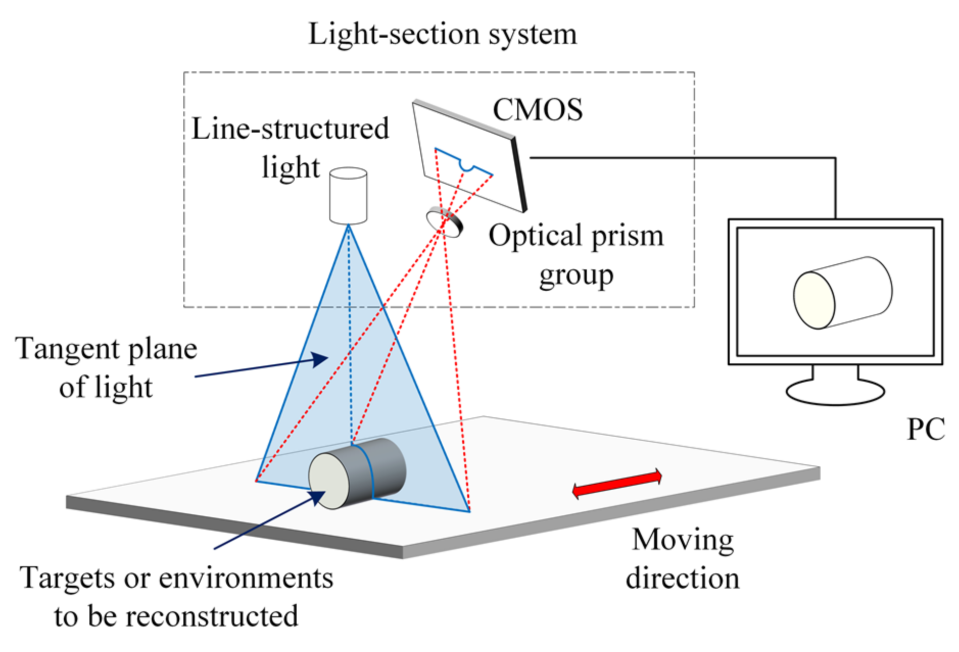
3.1. Principle of Laser Triangulation Measurement

Specific to 3D light-section reconstruction technology, the acquisition method of point cloud data is equivalent to the laser triangulation measurement, where the coordinates of each point need to be obtained through the laser stripe centerline extraction method. The optical structure of a typical triangulation measurement system, where the laser is incident on the vertical reference plane, and the Complementary metal oxide semiconductor (CMOS) is placed obliquely, is shown in Figure 5.

The original point is the intersection of the laser and the lens normal when the laser is incident perpendicular to the reference plane. The plane that passes through this point, which is also perpendicular to the laser line, is taken as the reference plane. The height h of the measured point of the object can be expressed as:

$$h=\frac{dL}{cos\alpha \left(lcos\alpha +dsin\alpha \right)}$$

(1)

where α is the angle between the reference plane and the line within the origin point and the center of the lens; l is the distance from the center of the lens to the imaging surface; d is the distance between the imaging position and the center of the CMOS; and L is the horizontal distance between the laser and the CMOS.

The coordinates of each point are connected according to the correct topological relationship to characterize the contour information of the measured object in the current section. Considering the accuracy, robustness, and versatility of the extraction process, the commonly used methods for extracting the centerline of laser stripes mainly include the gray centroid method, the Steger method, the Hessian matrix method, etc., which achieve micrometer-level sub-pixel extraction accuracy [10,11]. At present, the latest research in this field has made certain adjustments to the classic algorithms mentioned above for particular applications, which has not yet been a significant breakthrough in principle.

Subsequently, the whole system needs to be calibrated to map the extracted two-dimensional pixel coordinates into three-dimensional space in the correct sequence. The current laser triangulation measurement system mainly adopts the Scheimpflug imaging system, considering the high requirements for imaging clarity in the depth of field in 3D measurement. From a scale-invariant perspective, the Scheimpflug imaging process can be considered a non-linear mapping from one two-dimensional (2D) vector space, the original object plane, to a 3D imaging surface. This non-linear mapping will introduce nonrotational symmetric aberrations, a non-uniform resolution, a non-uniform intensity distribution, and other issues in the system that affect the measurement accuracy. Therefore, it is crucial to accurately determine the parameters of the mathematical model for the Scheimpflug measurement system to achieve a precise transformation between pixel coordinates and spatial positions [12].

There are three essential elements during the whole calibration process: the pixel coordinates, the real-world coordinates, and the corresponding transformation relationship. Focusing on these elements, existing studies on calibration methods can be divided into three categories.

The first extensively developed category of studies is those on Zhang’s camera calibration method, which can be classified as a plane method. However, the different model of the Scheimpflug measurement system with two inclination angles, where the lens is parallel to the image plane, means that Zhang’s method is not applicable. When this difference is ignored, the residual error for the calibration results may be much more extensive, leading to lower precision. Meanwhile, the results of fitting calibration may prefer local optimization rather than global optimization when separating the imaging part and the object plane part from the entire system to compensate for the deficiency of Zhang’s method [13]. This method can theoretically cause secondary error propagation, similar to the two-step calibration method, thus affecting the precision of the calibration results.

Another category is the physical calibration method studies that adopt an in-kind object on which the real-world coordinate system is built. This object must contain some known spatial relationships to provide details on the feature points that focus on obtaining a fitting function. Several past studies have used calibration boards or unique shapes of objects. Alternatively, these methods are limited by objective conditions, such as the calibration object and its processing accuracy, or perhaps by the high demands of the experimental environment and efficient parallel algorithm.

The last kind is the studies on the displacement method, where the final calibration accuracy can be traced back to the displacement corresponding to the necessary real-world coordinates. The calibrator adopted by these methods does not limit the processing accuracy, which completely resolves the drawbacks of the physical calibration method. Meanwhile, this method can achieve a minimal movement interval to obtain dense datasets compared with others to achieve higher accuracy than traditional calibration methods [14].

In addition, the depth information in the Z-axis will have an error accumulation phenomenon, which is difficult to eliminate through system calibration due to the limitation of the principle of the light-section 3D reconstruction technology. The current ideal solution to this problem is to perform scale transformation and fusion to obtain a directed point cloud after multiple measurements, which can be taken as high-precision original data.

3.2. Point Cloud Filtering and Decorating Methods

The original point cloud will produce outliers due to the inherent noise of the sensor or acquisition device, the surface characteristics of the objects, or other environmental/human factors, which will affect the accuracy of the 3D reconstruction. Therefore, it is essential to weaken or even remove noise on the basis of preserving the initial features and details of the point cloud. Point cloud filtering methods can be divided into seven categories:

• Statistics-based filtering methods;
• Neighborhood-based filtering methods;
• Projection-based filtering methods;
• Filtering methods based on signal processing;
• Filtering methods based on partial differential equations;
• Hybrid filtering methods;
• Other filtering methods.

The filtering methods for the point cloud are relatively consummate at present, and have also been introduced by some reviews [15]. Therefore, this paper will not give a detailed introduction and overview of this technology.

After filtering the original point cloud data, the holes caused by the missing data during the collection process or the visual blind zone in laser triangulation measurement can be viewed more clearly. These holes in semi-disordered point clouds will bring great difficulties to subsequent processing, such as non-convergence of the algorithm, errors in solving equations, failure of topological connection, etc. Especially for non-rigid objects or complex environments to be tested, the point cloud hole phenomenon is a problem that cannot be ignored. The current algorithms for hole repair, most of which are point cloud data amplification methods based on boundary equations, are relatively intuitive linear/non-linear fitting methods.

As shown in Figure 6, one of the classic point cloud datasets produced by Stanford University, which has been frequently adopted, is the Stanford Bunny [16].

4. Point Cloud Reduction Methods

Generally speaking, the front-end system requires a higher sampling rate and resolution, which results in an enormous amount of original data and a higher density of information space, to obtain a high-quality point cloud. The demand for point cloud data storage and related computing speeds is also increasing exponentially with the range expansion or the increasing complexity of the object to be reconstructed. However, the data volume of a filtered point cloud is still huge, with insufficient necessity. The inefficient storage, operation, and transmission of massive data directly affect the convergence of subsequent algorithms. In the case of low point cloud accuracy requirements, the point cloud density can be reduced by decreasing the sampling resolution. On the other hand, it is necessary to down-sample the data and establish a topological structure before further operations on the point cloud when the application scenario is high-precision object reconstruction.

Point cloud reduction methods can be divided into the following five categories.

4.1. Traditional Down-Sampling Reduction Methods

Traditional sparse down-sampling methods for point clouds mainly include the random down-sampling method, uniform down-sampling method, and point-spacing down-sampling method [17,18,19]. Among them, the random down-sampling method only needs to select a specific number of points from the original data; the uniform down-sampling method removes some of the points according to the order of insertion points; and the point-spacing down-sampling method completes the data screening based on the pre-specified minimum distance between adjacent points. Compared with the random down-sampling method, the other two down-sampling methods achieve a more uniform spatial distribution.

However, none of the three methods considers local surface features or point density changes in the original point cloud, leading to the loss of some details, making it challenging to achieve high-precision three-dimensional reconstruction. Existing research has shown that the point density does not affect subsequent recognition and modeling operations in a specific local neighborhood. Therefore, the local neighborhood in the above algorithm process can be randomly refined to obtain a higher local point density than the specified density to retain more details and achieve more accurate adaptive down-sampling. It is worth noting that the performance of the adaptive down-sampling method highly depends on the accurate local characterization process due to the need to estimate the point density [20].

Chen et al. gradually improved resampling quality by interleaving optimization for resample points and updating the fitting plane [21]. This general framework can generate high-quality resampling results with an isotropic or anisotropic distribution from a given point cloud.

In addition, Rahmani et al. selected a greedy method to find sampled data points for the problem that the minimization equation is nonconvex and difficult to solved in down-sampling [22]. The first embedding vector is randomly sampled during initialization. In the subsequent step, the next embedding vector is sampled to have the largest distance from the previously sampled embedding vector. Therefore, the other embedding vectors far away from the sampled embedding vector are taken as the target, where the sampled embedding vector gradually covers the distribution of all embedding vectors in each step.

Meanwhile, Al-Rawabdeh et al. proposed two improved down-sampling methods on this basis [23]. The first is a plane-based adaptive down-sampling strategy, which removes redundant points in a high-density area while keeping the points in a low-density area. The second method derives the normal surface vector of the target point cloud through the local neighborhood, which can be expressed on the Gaussian sphere, achieving down-sampling by removing the points through the detected peaks. Furthermore, Tao et al. and Li et al. adopted bi-Akima in the selective sampling of initial points [24,25].

4.2. Reduction Methods Based on Geometric Features

The second kind of method is to determine the weight of each point in the point cloud through geometric features, removing the less important points to achieve the purpose of streamlining the point cloud. Han et al. proposed an edge-preserving point cloud simplification algorithm based on normal vectors [26]. Particular edge points should always be retained in the process of point cloud simplification due to their more apparent characteristics than nonedged points. The algorithm first uses an octree to establish the spatial topological relationship of each point and then applies a simple but effective method to identify and retain edge points. Focusing on those non-edge points, the least essential points are deleted until the data reduction rate is reached. The importance of non-edge points is measured using the average Euclidean distance (based on the normal vector) of the estimated tangent plane from the point to each neighboring point.

Sayed et al. took advantage of an intelligent feature detection algorithm based on point sampling geometry to select the initial point, combined with Gaussian interpolation, to evaluate and select the remaining points until reaching a predetermined reduction level. This method overcomes the time complexity problem in the point cloud simplification process, which only sacrifices 0.7% of the accuracy [27].

Meanwhile, Xuan et al. adopted the local entropy based on the normal angle to evaluate the importance of points, which is derived on the basis of the normal angle and information entropy theory through the estimation of the normal vector. The point cloud is finally simplified by removing the least important points, which are evaluated by gradually updating the normal vector and the corresponding importance value [28].

In addition, Ji et al. proposed a simplified algorithm based on detailed feature points, which has different processes to achieve three aspects of improvement [29]. First, the k-neighborhood search rule is set to ensure that the target point is closest to the sample point so that the calculation accuracy of the normal vector is significantly improved and the search speed is greatly improved. Second, a vital measurement formula, considering multiple features, is proposed to preserve the main details of the point cloud. Finally, the octree structure simplifies the remaining points, significantly reducing the hole in the reconstructed point cloud.

In addition, Guo et al., Tazir et al., and Thakur et al., respectively, chose curvature, color, distance, and other information to reduce the point cloud data [30,31,32].

4.3. Reduction Methods Based on Component Analysis

The third type of method is to measure the structure and composition information of the point cloud from a global perspective. Markovic et al. proposed a simplified method for the sensitization of 3D point cloud features based on ε-insensitive support vector regression, which is suitable for structured point clouds [33]. The algorithm uses the flatness characteristics of the ε-support vector regression machine to effectively identify points in the high-curvature area, which are saved in a simplified point cloud along with a reduced number of points from a flat area. In addition, this method can effectively detect points near sharp edges without additional processing.

In addition, Yao et al. exploited dimensionality reduction technology to generate 2D data by extracting the first and the second principal components of the original data with minor information loss. The generated 2D data are clustered for noise reduction before being restored to 3D in the 2D space spanned by the two principal components. This method reduces computational complexity and effectively removes noise by performing dimensionality reduction and clustering on generated 2D data while retaining details of environmental features [34].

4.4. Reduction Methods Based on Spatial Subdivision

The fourth type of method is adopting spatial subdivision to achieve point cloud down-sampling. El-Sayed et al. took advantage of an octree to subdivide the point cloud into small cubes with a limited number of points, which were down-sampled according to the local density of each cube [35]. Song et al. also applied the octree encoding method to divide the neighborhood space of the point cloud into multiple sub-cubes with specified side lengths, which kept the closest point of each sub-cube from the center point to simplify the point cloud [36]. Lang et al. used adaptive cell-sized voxel grids to characterize point clouds, which down-sampled the point clouds by finding the centroid of each grid [37].

In addition, Shoaid et al. resorted to a fractal bubble algorithm to generate a 2D elastic bubble and a copy of itself through a 2D dataset representing the geometric contour of a plane. As the bubbles grow, each bubble will select a single point that it first touches, which will become a simplified set of points. The fractal bubble algorithm is repeatedly applied to simplify the plane slices of the general 3D point cloud corresponding to the 3D geometric object, resulting in global simplification of the 3D point cloud [38].

4.5. Reduction Methods Based on Deep Neural Networks

The fifth category of methods combines deep learning and neural networks, while deterministic down-sampling of disordered point clouds in deep neural networks has not been rigorously studied so far [39]. Existing methods down-sample the points regardless of their importance to the network output. Therefore, some critical points may be removed, and lower value points may be transported to the next layer. Furthermore, it is necessary to sample points by considering the importance of each point, which varies according to the application, task, and training data.

Xin et al. introduced the data simplification and point retention steps based on neural networks in the contour area of the point cloud between the coarse alignment process of the model data with the measured data as well as the precise registration process of the reweighted iterative closest point algorithm, which significantly reduced the complexity of time and space and improves computational efficiency without loss of accuracy [40].

In addition, Nezhadarya et al. proposed a new deterministic, adaptive, and unchanging down-sampling layer called the critical point layer, which learns to reduce the number of points in the disordered point cloud while retaining the important (critical) point [41]. Unlike most graph-based point cloud down-sampling methods, the graph-based down-sampling methods use K-nearest neighbor (K-NN) to find neighboring points. At the same time, the critical points layer (CPL) is a global down-sampling method, which computational efficiency is very high. The proposed layer can be developed with a graph-based layer to form a convolutional neural network.

5. Point Cloud Registration Methods

Limited by the principle of structured light measurement and the development direction of multi-source data fusion, it is usually necessary to synthesize multiple sets of point cloud data and register point clouds in different world coordinate systems to the same coordinate system to complete high-precision reconstruction of objects or the environment, which is called point cloud registration. The main difficulties of the current registration process include:

• The point cloud density inconsistent, caused by different distances and perspectives of data acquisition sources, or the overlap rate between multiple sets of point clouds being lower, making it difficult to converge the registration algorithm;
• Self-similar or symmetric objects can easily cause misregistration in the absence of practical constraints;
• Loss of point cloud data caused by occlusion in a complex environment makes the registration process lack valid input;
• The noise or outliers introduced in the data acquisition process make the iterative direction not unique and prone to phenomena such as “artifacts”;
• A large number of point clouds in a single time leads to a large amount of calculation, increased time-consuming, and lower time efficiency.

Traditional point cloud registration methods mainly rely on explicit neighborhood features such as curvature, point density, and surface continuity. The details of the object are easily lost in the subdivision area with sudden curvature. Most of the improvements in such algorithms are to find suitable registration features, speed up data queries, and optimize registration efficiency. Some of the registration methods require a higher initial position of the cloud point, which easily falls into the local optimum and makes it challenging to obtain a good registration result when the overlap rate between two point clouds is high.

The following is a detailed introduction of various classical registration methods and the latest related research, with a brief summary of classical algorithms in

Table 2. A brief summary of classical registration methods.

Category	Algorithm Name	Author	Year	Keywords
Based on mathematical solutions	——	——	——	Rotation transformation matrix; Translation transformation matrix
Based on statistical models	RANSAC [42,43]	Fischler and Chen	1981–1991	Random sample consensus
	NDT [44]	Biber	2003	Normal distributions transform
	4PCS [45]	Aiger	2008	Four coplanar points; RANSAC
	CPD [46]	Myronenko	2010	Coherent point drift
Based on point cloud features	Spin-Images [47]	Johnson	1997	Cylindrical-coordinate system
	HIS [48]	Zhang	1999	Harmonic shape images
	3Dsc [49]	Frome	2004	3D shape context
	SHOT [50]	Salti	2004	Signature of histogram of orientation
	PFH [51]	Rusu	2008	Persistent feature histograms
	FPFH [52]	Rusu	2009	Fast persistent feature histograms
	VFH [53]	Rusu	2010	Viewpoint feature histogram
	HKS [54]	Sun	2009	Heat kernel signature
	PPF [55]	Drost	2010	Point pair feature
Based on ICP deformation	ICP [56]	Besl	1991	Iterative closest point
	IDC [57]	Lu	1997	Iterative dual correspondences
Based on deep learning	LORAX [58]	Elbaz	2017	Localization by registration using a deep auto-encoder reduced cover set

.

5.1. Registration Methods Based on Mathematical Solutions

The mathematical expression of the point cloud registration process is to solve the rotation and translation matrix (rigid transformation condition or Euclidean transformation condition) between multiple point clouds, as shown in the formula:

$$p_t=\mathit{R}·p_s+\mathit{T}$$

(2)

where p_t and p_s are a set of corresponding points between the target point cloud and the original point cloud. R and T are the rotation transformation matrix and the translation transformation matrix, respectively. As a result, the point cloud registration process can be transformed into a mathematical model solving problem.

Jauer et al. solved the registration problem by assuming that the point cloud is a rigid body composed of particles based on principles of mechanics and thermodynamics [59]. Forces can be applied between two particle systems to make them attract or repel each other. These forces are used to bring about rigid movement between particle systems until the two are aligned. This framework supports a physically based registration process, with arbitrary driving forces depending on the desired behavior.

Meanwhile, de Almeida et al. expressed the rigid registration process by comparing it with the coding of the intrinsic second-order direction tensor of local geometry. Therefore, the applied Gaussian space can have a Lie group structure, which can be embedded in the linear space defined by the Lie algebra of the symmetric matrix, to be adopted in the registration process [60].

Parkison et al. exploited a new regularized model in the regenerative kernel Hilbert space (RKHS) to ensure that the corresponding relationship is also consistent in the abstract vector space (such as the intensity surface). This algorithm regularizes the generalized iterative closest point (ICP) registration algorithm under the assumption that the intensity of the point cloud is locally consistent. Learning the point cloud intensity function from the noise intensity measurement instead of directly using the intensity difference solves possible mismatch problems in the data association process [61].

In addition, Wang et al. proposed a set of satisfactory solutions for the Cauchy mixture model, using the Cauchy kernel function to improve the convergence speed of the registration [62]. For rigid and affine registration, the calculation of the Cauchy mixture model is more straightforward than that of the Gaussian mixture model (GMM), which requires less strict correspondence and initial values. Feng et al. proposed a point cloud registration algorithm based on gray wolf optimizer (GWO), which uses a centralization method to solve the translation matrix. Subsequently, the inherent shape features are employed to simplify the points of the initial point cloud model, and the quadratic sum of the distances between the corresponding points in the simplified point cloud is utilized as the objective function [63]. The various parameters of the rotation matrix are obtained through the GWO algorithm, which effectively balances the global and local optimization ability to obtain the optimal value in a short time.

In addition, Shi et al. introduced the adaptive firework algorithm into the coarse registration process, which reminds us that multiple types of optimization algorithms can be applied in the point cloud registration process to achieve higher precision [64].

5.2. Registration Methods Based on Statistical Models

The robust model estimation method that Fischler et al. proposed in 1981 can handle a large number of outliers, namely Random Sample Consensus (RANSAC), is one of the classic registration algorithms in the field of computer graphics [42]. Chen et al. applied the RANSAC idea to the point cloud data registration process in 1991 [43], the process of which is:

Step 1: Randomly find three non-collinear points in the original point cloud P_s and three corresponding points in the target point cloud P_t. The transformation matrix H_k between two point clouds is estimated through these point pairs;

Step 2: Calculate the degree of agreement between the remaining point pairs of the original point cloud p_s and the target point cloud p_t under the transformation matrix H_k and the error threshold δ obtained in step 1;

Step 3: Iteratively carry out step 1 and step 2 until the transformation matrix H with the greatest degree of correspondence between the original point cloud p_s and the target point cloud p_t is found, which is the transformation matrix between two point clouds obtained in the registration process.

In summary, the RANSAC algorithm, having a certain probability of obtaining the correct result, estimates the model parameters for samples containing outliers in an iterative manner. Moreover, the time complexity of this algorithm is high, which makes it difficult to apply in large-scale point clouds. In addition, the effect of the RANSAC algorithm is relatively poor when the point cloud overlap rate is low, or the proportion of outliers is high.

In 2008, Aiger et al. proposed the 4-Points Congruent Sets (4PCS) algorithm, using four coplanar points as RANSAC search elements on this basis [45]. This method is robust and fast in search speed, which has the ability to handle arbitrary initial position alignment through the introduction of constraint invariants. However, the disadvantage of this type of method is that there are certain restrictions on the surface shape of the point cloud to be registered. The registration result is poor if the overlap rate between point clouds is very low (less than 20%) and the overlap is concentrated in a relatively small area of the point cloud. Improvements to the algorithm include Super 4-Points Congruent Sets (Super4PCS), Multiscale Sparse Features Embedded 4-Points Congruent Sets (MSSF-PCS), Volumetric 4-Points Congruent Sets (V4PCS), etc. [65,66,67].

In addition, Hähnel et al. proposed another probabilistic registration algorithm in 2002 [68]. The algorithm regards the measured value of the reference scan as a probability function, calculating the probability density of each pair of scans, to perform registration through a greedy hill-climbing search in the likelihood space. Boughorbel et al. used the Gaussian mixture model in 2004 to measure the spatial distance between the two scan points and the similarity of the local surface around the point to achieve registration [69].

Attempting to solve the problems of low time efficiency of the traversal and error-prone feature matching process, Biber et al. proposed an normal distributions transform (NDT) registration method in 2003 [44]. The algorithm divides the space into several cells and calculates the parameters of each cell according to the distribution of points in the cell. Then, another point cloud is transformed according to the transformation matrix T to obtain the response probability density distribution function in the corresponding cell, as shown in the formula of the likelihood of having measured $\overrightarrow{x}$:

$$p\left(\overrightarrow{x}\right)=\frac{1}{{(2\pi )}^{D/2}\sqrt{\left|\mathsf{\Sigma }\right|}}\exp \left(-\frac{{(\overrightarrow{x}-\overrightarrow{\mu })}^{\mathrm{T}}{\Sigma }^{-1}\left(\overrightarrow{x}-\overrightarrow{\mu }\right)}{2}\right)$$

(3)

where $\overrightarrow{\mu }$ denotes the mean vector and covariance matrix of the reference scan surface points within the cell where $\overrightarrow{x}$ lies. The optimal value of all points for the objective function is obtained, which is the rotation and translation matrix corresponding to the registration result that maximizes the likelihood function:

$$\mathsf{\Psi }={\displaystyle \prod }_{k=1}^{n}p\left(T\left(\overrightarrow{p},{\overrightarrow{x}}_k\right)\right)$$

(4)

where $\overrightarrow{p}$ encodes the rotation and translation of the pose estimate of the current scan. The current scan is represented as a point cloud $\chi =\left\{{\overrightarrow{x}}_1,\dots ,{\overrightarrow{x}}_n\right\}$. A spatial transformation function $T\left(\overrightarrow{p},\overrightarrow{x}\right)$ moves a point $\overrightarrow{x}$ in space by the pose $\overrightarrow{p}$.

However, the registration accuracy of NDT largely depends on the degree of cell subdivision. Determining the size, boundary, and distribution status of each cell is one of the directions for the further development of this type of algorithm.

In addition, Myronenko et al. proposed a coherent point drift (CPD) algorithm in 2010, which regarded the registration as a probability density estimation problem [46]. The algorithm fits the GMM centroid (representing the first point cloud) with the data (the second point cloud) through maximum likelihood. In order to maintain the topological structure of the point cloud at the same time, the GMM centroids are forced to move coherently as a group. In the case of rigidity, the Expectation Maximum (EM) algorithm’s maximum step-length closed solution in any dimension is obtained by re-parameterizing the position of the centroid of the GMM with rigid parameters to impose coherence constraints, which realizes the registration.

Focusing on the problem that too many outliers will cause significant errors in estimating the log-likelihood function, Korenkov et al. introduced the necessary minimization condition of the log-likelihood function and the norm of the transformation array into the iterative process to improve the robustness of the registration algorithm [70].

Li et al. borrowed the characteristic quadratic distance to characterize the directivity between point clouds. By optimizing the distance between two GMMs, the rigid transformation between two sets of points can be obtained without solving the correspondence relationship [71]. Meanwhile, Zang et al. first considered the measured geometry and the inherent characteristics of the scene to simplify the points [72]. In addition to the Euclidean distance, geometric information and structural constraints are incorporated into the probability model to optimize the matching probability matrix. Spectrograms are adopted in structural constraints to measure the structural similarity between matching items in each iteration. This method is robust to density changes, which can effectively reduce the number of iterations.

Zhe et al. exploited a hybrid mixture model to characterize generalized point clouds, where the von Mises–Fisher mixture model describes the orientation uncertainty and the Gaussian mixture model describes the position uncertainty [73]. This algorithm combined the expectation-maximization algorithm to find the optimal rotation matrix and transformation vector between two generalized point clouds in an iterative manner. Experiments under different noise levels and outlier ratios verified the accuracy, robustness, and convergence speed of the algorithm.

In addition, Wang et al. utilized a simple pairwise geometric consistency check to select potential outliers [74]. Transform and decomposition technology is adopted to estimate the translation between the original point clouds for a set of potential internal correspondence pairs. Meanwhile, a rotation search algorithm based on the correspondence relationship estimates the rotation between the two original point clouds. The translation and rotation search algorithms are based on the Branch-and-Bound (BnB) optimization framework, which means that the corresponding input data are globally optimal. However, the optimal solution of the two decomposition problems of the three-degree-of-freedom (DoF) translation search and the 3DoF rotation search is not necessarily the optimal solution of the original 6DoF problem of rigid registration. Experiments showed that the accuracy of the registration is acceptable.

5.3. Registration Methods Based on Point Cloud Features

The use of mathematical solutions or traversal-exhaustive ideas to achieve registration between point clouds has certain limitations on computational efficiency, which is difficult to be actually applied to the registration process of large-scale point clouds. Low-dimensional point feature information such as normal surface vectors and local curvatures was adopted to simplify the amount of input data for the point cloud registration process in the early years of the research.

Johnson et al. proposed a Spin-Images descriptor in 1997 to generate a cylindrical coordinate system based on feature points and their normal vectors [47]. The three-dimensional coordinates in the cylinder are projected into the two-dimensional image, and the corresponding intensity is calculated according to the points that fall in each image grid, which forms the Spin-Images descriptor. The registration method based on this feature quantity does not require any attitude measurement hardware or manual intervention, nor does it need to assume any prior knowledge of the initial position or dataset overlap to complete the registration of the three-dimensional point cloud. Relying on Spin-Images’ robustness to occlusion and clutter, as well as the rotation and translation invariance, this method can also obtain satisfactory results for the registration of cluttered and occluded three-dimensional point clouds.

In 1999, Dongmei et al. constructed harmonic mapping through a two-step process of boundary mapping and internal mapping so that there is a one-to-one correspondence between the points on the 3D surface and the mapped image. While preserving the shape and continuity of the primary surface, a general framework is adopted to represent surface properties such as normal vectors, colors, textures, and materials, which are called harmonic shape images (HSI) descriptors [48].

These kinds of algorithms have improved the calculation speed to a certain extent. While it is difficult to distinguish some local features with high similarity, and the registration effect between point clouds with the inconsistent resolution is poor. Therefore, researchers introduced high-level feature information to characterize discrete point clouds, which achieved rapid registration between point clouds by matching three-dimensional or multi-dimensional feature information. Current research on feature descriptors mainly focuses on the local rather than global level because local feature descriptors can resist interference such as chaos and occlusion, while global feature descriptors are more sensitive to clutter and occlusion.

Frome et al. proposed a descriptor called 3D shape context (3Dsc) in 2004 [49]. This method adopts the normal vector of the key point as the local reference axis, where the spherical neighborhood is equally divided along the azimuth and elevation dimensions. Meanwhile, the radial dimension is divided logarithmically. The 3Dsc descriptor is generated by counting the number of weighted points that fall into each area.

Meanwhile, Rusu et al. proposed persistent feature histograms (PSH) descriptors in 2008, which consider all interactions between the estimated normal directions by parameterizing the spatial difference between the query point and the neighboring point [51]. The algorithm attempts to capture the best sample changes of the surface to describe the geometric characteristics of the sample, which forms a multi-dimensional histogram for the description of the geometric attributes of the k-neighborhood of the point. The highly dimensional hyperspace located in the histogram provides a measurable information space for feature representation, which is invariant to the six-dimensional posture of the corresponding surface of the point cloud. This method is robust under different sampling densities or neighborhood noise levels.

Specifically, the point-to-coordinate system constructed in the point cloud is:

$$\left\{\begin{array}{c}u=n_s\\ v=u\times \frac{\left(p_t-p_s\right)}{\Vert p_t-p_s\Vert {}^2}\\ w=u\times v\end{array}\right.$$

(5)

where vectors u, v and w are the computed Darboux frame. $p_s$ is defined as the source point and $p_t$ is defined as the target point. $n_s$ is the estimated normal at point of $p_s$.

Meanwhile, the representation based on the neighborhood feature is shown in the formula:

$$\left\{\begin{array}{c}\begin{array}{c}\alpha =v·n_t\\ \varnothing =u·\frac{\left(p_t-p_s\right)}{d}\end{array}\\ \begin{array}{c}\theta =arctan\left(w·n_t, u·n_t\right)\\ d=\Vert p_t-p_s\Vert {}_2\end{array}\end{array}\right.$$

(6)

where <α, φ, θ, d> are a measure of the angles between the points’ normals and the distance vector between them. $n_t$ is the estimated normal at point of $p_t$.

However, the time complexity of calculating the PFH feature for a query point is O(k²). The time complexity is O(nk²) if a point cloud has n points, which has extremely low efficiency. R.B. Rusu et al. improved it into an fast persistent feature histogram (FPFH on this basis in 2009 [52]. Meanwhile, the weighted average of the statistics of the point pairs was taken in the k neighborhood, as shown in the formula:

$$FPFH\left(p_q\right)=SPFH\left(p_q\right)+\frac{1}{k}{\displaystyle \sum }_{i=1}^k\frac{1}{w_k}· SPFH\left(p_k\right)$$

(7)

where simplified point feature histogram (SPFH) simplifies <α, φ, θ, d> to <α, φ, θ>. The weight $w_k$ represents the distance between query point p and a neighbor point $p_k$ in a given metric space.

FPFH retains most of the information of FPH, which has pose invariance and strong description ability to shorten the calculation time in the registration process considerably. Rusu et al. also introduced perspective features based on FPFH in 2010, called the viewpoint feature histogram (VFH) descriptor [53]. Beyond implementing the registration function, this descriptor better meets the functional requirements for recognition and pose estimation.

In 2009, Sun et al. proposed a shape-based thermal diffusion characteristic descriptor, which is called thermonuclear features heat kernel signature (HKS) [54]. This algorithm calculates the residual heat of each point in the point cloud over time, which is the corresponding curve between the degree of heat diffusion and the passage of time. The algorithm adopted this as the hot core feature of the point to realize the point cloud registration through the search and matching processes, which has certain robustness, while only being suitable for application scenarios under equidistant changes. Meanwhile, Zobel et al. proposed the general heat kernel signature (GHKS) descriptor in 2011 and 2015, which supplements and improves this type of algorithm [75].

On the other hand, Drost et al. proposed a point pair feature (PPF) descriptor in 2010 to represent the relative position and attitude of two directed points [55]. The set of feature vectors and the point pair set corresponding to each feature vector was built into a global model of the point cloud. Pick any point in the model to match the position and normal vector of a certain point in the target point cloud. Then, the optimal number of matching point pairs between two point clouds is found through voting, etc., which means the registration is successful. The algorithm can be applied in environments with interference, stacking, partial occlusion, etc.

In 2004, Salti et al. proposed the signature of histogram of orientation (SHOT) descriptor to seamlessly integrate multiple data source information, which adopted the structure of feature signatures and histograms to improve the uniqueness, descriptiveness, and robustness of the descriptor [50]. Specifically, the feature signature encodes local spatial geometric information by defining the local reference frame (LRF). The eigenvalues of its local geometric space are ordered due to the existence of the LRF. The histogram divides the eigenvalues into intervals, which were encoded in the manner of histogram statistics so that the statistics were disordered. The spherical support area is divided into 32 partitions as shown in Figure 7, performing quadrilinear interpolation in the dimensions of normal vector cosine, longitude, latitude, and radial, which weakens the edge effect and completes the characterization of the space.

In recent years, researchers have implemented a lot of improvement work based on the above algorithm. Ahmed et al. exploited the quadratic polynomial of three variables to represent the area as an implicit quadric. The intersection of all three implicit quadric surfaces defines a virtual point of interest, representing a stable area in the point cloud. The algorithm reduces the computational cost of registration, which is robust to noise and data density changes [76].

Liu et al. established the local correlation of feature information based on the fast point feature histogram, combining with greedy projection triangulation [77]. Then, the sample consistency initial alignment method was applied to perform the initial transformation to achieve the initial registration. Experimental results show that greedy projection triangulation improves the accuracy and speed of registration, significantly improving the efficiency of feature point matching.

Sheng et al. used asymmetric coding, which cannot be affected by rotation, translation, and scale factors, to obtain plane boundary lines through Freeman differential coding and Hough transform [78]. This method constructed a two-level index structure, which greatly improved the feature matching efficiency and precision for the point cloud centerline.

Moreover, Truong et al. applied semantic information to point cloud registration, effectively deleting mismatched point pairs, ensuring maximum consistency in the registration process, and improving registration speed based on registration performance [79].

In addition, Zou et al. proposed a new local feature descriptor called the local angle statistical histogram (LASH) for effective 3D point cloud registration [80]. LASH encodes its characteristics at the angle between the normal vector of a point and the vector formed by other points in its local neighborhood to form a geometric description of the local shape. Then, triangle matching points are detected with the same similarity ratio, which is adopted to calculate multiple transformations between the two point clouds.

Yang designed the corresponding hybrid feature representation for the point cloud carrying color information [81]. The weight parameter can be dynamically adjusted between the color and spatial information through the similarity measurement to more reliably establish the corresponding relationship in the point cloud and estimate the conversion parameters.

To reduce the influence of noise and eliminate outliers, Wan et al. established a registration model based on the maximum entropy criterion [82]. The algorithm introduces two-way distance measurement into the registration framework to avoid the model from falling into local extremes, which is highly robust.

Eslami et al. resorted to a feature-based fine registration method for images and point clouds [83]. The connection point and its two adjacent pixels are matched in the overlapping image, which intersects in the object space to create a differential connection plane. The initial rough external direction parameters (EDP), IOP internal direction parameters (IOP), and additional parameters (AP) are adopted to convert the connection plane points into object space. Then, the closest point between the point cloud data and the transformed contact plane point is estimated, which is used to calculate the direction sector of the different planes. As a constraint equation and a collinearity equation, each spatial contact point of an object must be located on the differential plane of the point cloud.

5.4. Registration Methods Based on ICP Deformation

The point cloud registration process can be divided into coarse registration and fine registration. The approximate rotation and translation matrix can be solved by the coarse registration algorithm when the relative position of each point cloud datum is unknown. The fine registration process takes the solution obtained by the coarse registration process as the initial value on this basis. Iterative optimization is performed by setting different constraint conditions, while the global optimal rotation and translation matrix solution is obtained to achieve higher precision registration.

The ICP algorithm and its variants are currently the most classic and commonly used precision registration methods [56], which progress is:

Step 1: Obtaining point pairs (nearest neighbor point). A transformed point cloud is obtained from the original point cloud, using the result of the rough registration process as the initial value. The point pair called the nearest neighbor point, whose distance between the point cloud and the target point cloud is less than a certain threshold, is the corresponding point between the point clouds.

Step 2: R, T optimization. Minimize the objective function through many corresponding points to obtain the optimal rotation and translation matrix. The m solution process is shown in the formula:

$${\mathit{R}}_{\mathit{m}}{}^{*},{\mathit{T}}_{\mathit{m}}{}^{*}=\arg \underset{R,T}{\min }\frac{1}{\left|P_s\right|}{\displaystyle \sum }_{i=1}^{\left|P_s\right|}\Vert P_t{}^i-{\left(\mathit{R}·P_s{}^i+\mathit{T}\right)\Vert }^2$$

(8)

where R, T is the corresponding initial value before the m solution, P_s, P_t is the corresponding point (nearest point) in the original point cloud and the target point cloud.

Step 3: Iterative re-optimization. The new R and T parameters are generated in step 2 cause some point pairs to change, which means the initial value of the iteration is inconsistent with the previous iteration. Therefore, Step 1 and Step 2 need to be continuously iterated until the preset iteration termination conditions are met, such as the relative distance change of the nearest point pair, the change in the objective function value, or the change in R and T less than a certain threshold.

The prerequisite for applying the ICP algorithm is that the original point cloud and the target point cloud are basically in a pre-aligned state. The registration process will usually fail due to falling into a local minimum if the point clouds are far apart or contain repetitive structures. In addition, the direct use of the ICP method is inefficient and unstable due to the difference between the point cloud density distribution, the acquisition scanner, and the scanning angle. At present, scholars have made specific improvements to the ICP algorithm based on the above problems.

In 1997, Lu et al. extended the ICP algorithm to the Iterative Dual Correspondences (IDC) algorithm, which accelerates the convergence of the rotating part in the attitude estimation during the matching [57].

Moreover, Ji et al. used a genetic algorithm to transform the point cloud to the vicinity of the 3D shape to realize the coarse registration of the point cloud in response to the requirement that the ICP algorithm needs a more accurate iterative initial value. Combined with the fine registration algorithm, this method improves the registration rate, matching accuracy, and convergence speed [84]. Bustos et al. presented a point cloud registration preprocessing method that guarantees the removal of abnormal points, which reduces the input to a small set of points in a way that rejects the correspondence relationship and ensures that it does not exist in the global optimal solution. In this way, the true outliers are deleted. At the same time, pure geometric operations ensure the accuracy and speed of the algorithm [85]. Liu et al. combined the simulated annealing algorithm and Markov chain Monte Carlo to improve the sampling and search capabilities in the point cloud, which achieves global optimization under any given initial conditions with the ICP algorithm [86].

In addition, Wang et al. proposed a parallel trimming iterative closest point (PTrICP) method for the fine registration of point clouds, which adds the estimation of the parallel overlap rate during the iterative registration process to improve the robustness of the algorithm [87]. Focusing on the rigid registration problem with noise and outliers, Du et al. introduced the concept of correlation and proposed a new energy function based on the maximum correlation criterion, which convergences monotonically from any given parameter with higher robustness [88].

5.5. Registration Methods Based on Deep Learning

The registration of point clouds combined with deep learning technology has been one of the emerging development directions in recent years. Elbaz et al. proposed a registration algorithm between a large point cloud and a short-range scanning point cloud, called the Localization by Registration Using a Deep Auto-Encoder Reduced Cover Set (LORAX) algorithm [58]. The algorithm uses a sphere as the basic unit to subdivide the point cloud into blocks and project them into a depth map. Adopting deep neural network-based autoencoder technology combined with unsupervised machine learning, the low-dimensional descriptor of the 5 × 2 matrix is calculated, which can realize the solution of the coarse registration conversion matrix of the point cloud.

Chang et al. adopted two consecutive convolutional neural network models to build a point cloud registration framework [89]. Based on the calculated average after training, the framework can estimate the conversion between the model point cloud and the data point cloud. Compared with the omnidirectional uncertainty covered by the first model, the second model can accurately estimate the direction of the 3D point cloud. Experimental results show that the framework could significantly reduce the estimation time while ensuring the accuracy of registration.

Furthermore, Perez-Gonzalez et al. proposed a deep neural network based on sparse autoencoder training, combined with the Euclidean and Mahalanobis distance map point registration learning method [90]. The algorithm does not assume the proximity between point clouds or point pairs, which is suitable for point clouds with high displacement or occlusion. Moreover, this algorithm does not require an iterative process and estimates the point distribution in a non-parametric manner, with a broader application range.

Weixin et al. trained an end-to-end learning point cloud registration network framework called Deep Virtual Corresponding Points (DeepVCP), which generates key points based on the learned matching probabilities between a set of candidate points. This method can avoid interference with dynamic objects and adopts the help of sufficiently prominent features in static objects to achieve high robustness and high registration accuracy [91].

In addition, Kurobe et al. built a deep learning-based point cloud registration system called CorsNet (Correspondence Net), which connects local features with global features and returns the correspondence between point clouds instead of directly setting or gathering features. Thus, it integrates more helpful information than traditional methods. Experiments showed that CorsNet is more accurate than the classic ICP method and more accurate than the recently proposed learning-based PointNetLK (PointNet framework based on Lucas and Kanade) and DirectNet (domain-transformation enabled end-to-end deep convolutional neural network), including visible and invisible categories [92].

6. Three-Dimensional Shape Representation Methods

The traditional shape representation process is primarily based on point-to-point correspondence. In 2000, Pfister et al. used point primitive surfels without direct connectivity to characterize geometric surfaces. The attributes of surfels include depth, texture color, normal, etc., which can be reconstructed on the screen space to achieve low-cost rendering [93]. However, the coherence of each primitive is poor, which is reflected in the discontinuity of the rendering surface.

In 2001, Zwicker et al. gave each footprint a Gaussian filter kernel with symmetric radius based on the surfels correlation algorithm, where the continuous surface was reconstructed by a weighted average [94]. The algorithm provides high-quality anisotropic texture filtering, hidden surface removal, edge anti-aliasing, and independent transparency. The method is less efficient when drawing highly complex models.

Rusinkiewicz proposed a grid algorithm QSplat, which is suitable for large-scale point clouds with low computational consumption in 2000, since traditional grid display, simplified and progressive transmission algorithms are difficult to adopt in the situation of increasing high-level point cloud data [95]. The algorithm combines the multi-resolution hierarchy based on the bounding sphere with the point-based rendering system for data culling, level of detail selection, and rendering. In addition, this algorithm makes the corresponding trade-offs in quantization, storage form, and description of the Splat shape, which has a faster rendering speed.

However, the feature point search is usually affected by image noise, distortion, light and shadow changes, etc., leading to image aliasing. In addition, point-based reconstruction ignores the structural information between sample points on the surface of the object, which introduces more difficulties for the subsequent processing of reconstructed points. In order to avoid the problems mentioned above, researchers have tried to reconstruct the three-dimensional scene using curves and curved surfaces.

The following is a detailed introduction to various classical 3D shape representation methods and the latest related research, with a brief summary of representation algorithms, as shown in

Table 3. A brief summary of classical representation methods.

Category		Algorithm Name	Author	Year	Keywords
Parametric shape representation		Coons [96]	Coons	1964–1967	Four boundaries of a closed curve
		Bezier curve [97]	Bezier	1971	——
		B-spline curve [98]	Gordon	1974	——
		NURBS [99]	Versprille	1975	Non-uniform rational B-spline curve
		BPLI [100]	Barequet	1996	Piecewise-linear interpolation
Implicit surface representation	Global	RBF [101,102]	Hardy	1971	Radial basis function
		PSR [103]	Kazhdan	2006	Poisson surface reconstruction
		SPSR [104]	Kazhdan	2013	Screened poisson surface reconstruction
	Local	MLS [105]	Lancaster	1981	Moving least squares
		MTLS [106]	Scitovski	1998	Moving total least squares
		MPU [107]	Ohtake	2003	Multi-level partition of unity implicits
		APSS [108]	Guennebaud	2007	Algebraic point set surfaces
		RIMLS [109]	Öztireli	2009	Robust implicit moving least squares
		PIA [110]	Hamza	2020	Progressive iterative approximation
Mesh representation		LTA/FA [111]	Lawson	1977	Local transformation algorithm
		B-W A [112,113]	Bowyer, Watson	1981	Triangulation of an m-dimensional space point set
		TGM [114,115,116,117]	Brassel, Mirante, Green	——	Triangulation growth method
		Crust [118]	Amenta	1998	Vertices of the Voronoi diagram
		Co-cone [119]	Amenta	2000	Simplification of Crust
		BPA [120]	Bernardini	1999	Ball pivoting algorithm
Voxel representation		MC [121]	Lorensen	1987	Marching cubes
		MTA [122]	Doi	1991	Marching tetrahedral algorithm
Other representation methods		Surfels [93]	Pfister	2000	Include depth, texture color, normal
		QSplat [95]	Rusinkiewicz	2000	Multi-resolution hierarchy

.

6.1. Parametric Shape Representation Methods

Parametric shape representation can also be referred to as explicit shape representation, representing the three-dimensional surface in the point cloud using realizable parameters. This type of algorithm is simple in principle and intuitive to implement, which is susceptible to the limitation of original data to characterize the occluded part of the data with less flexibility. The various algorithms for parametric shape representation are introduced below.

In the process of parameter characterization, the most classic idea is to complete the feature surface drawing of the original point cloud by inserting points and connecting lines to form a surface. Coons first proposed a universal surface description method in 1964–1967 to define a curved surface, given four boundaries of a closed curve. However, this method requires a large amount of data, and there are certain uncontrollable factors in the shape and connection of the curved surface [96].

In response to the method mentioned above, Bezier proposed a way to modify the shape of the curve by controlling the position of the vertex, which formed the Bezier curve and surface technology after development and perfection [97]. This method is simple to calculate, and the reconstructed surface is controllable, while it still cannot meet the requirements of surface connection and local modification. Therefore, Gordon et al. proposed the B-spline curve and surface method in 1974, which solved the problems of local control and parameter continuity while retaining the advantages of Bezier theory [98]. However, this algorithm cannot accurately represent conic section lines and elementary analytical surfaces, limiting application scenarios.

Versprille extended the non-rational B-spline method to four-dimensional space in 1975, forming the current mainstream non-uniform rational B-spline curve (NURBS) algorithm [99]. NURBS curves can accurately represent standard analytical shapes, such as simple algebraic curves and surfaces, which can also represent various forms of free-form curves and surfaces. Meanwhile, NURBS has geometric invariance under affine, translation, shear, parallel and perspective projection transformations. Therefore, the algorithm has relatively loose requirements for the initial value, which reduces the computing demand.

In 1992, Meyers proposed an algorithm to reconstruct the surface from the contour structure, which comprehensively dealt with four problems in the process of extending from the “line” to the “surface” as follows; (1) The correspondence between the contour line and the surface; (2) the tiling problem of each contour; (3) the apparently divergent ruling issue; and (4) the optimal direction of the reconstructed surface [123]. Barequet et al. proposed an optimal triangulation strategy based on a dynamic programming algorithm for this problem in 1996, which is called (Barequet’s Piecewise-Linear Interpolation (BPLI) algorithm. The segmentation result that conforms to the actual topology can be obtained by connecting the input two-layer contour lines to a three-dimensional surface without self-intersection [100].

Scholars have made certain improvements on the basis of these classic algorithms, proposing methods such as bicubic Hermite interpolation, the bicubic Bezier surface method, the bicubic B-spline method, the least square surface method, the Legendre polynomial interpolation method, etc. [124,125,126,127,128].

Kong et al. adopted the discrete stationary wavelet transform method to extract the feature points of the surface to be reconstructed, which are the input data of the NURBS equation. Compared with the traditional NURBS surface reconstruction method, the root mean square error of the fitting result is reduced to 77.64% [129].

In addition, the newly proposed T-spline theory overcomes some of the topological constraints of the B-spline and NURBS, significantly reducing the number of control parameters, which has certain application prospects due to the linear independence and unity of the basis functions. For example, Wang et al. adaptively constructed a T grid suitable for the initial analysis according to the distribution of high-curvature feature points, where, to perform its local refinement and optimization, algorithms were run iteratively until the preset accuracy conditions were met [130].

6.2. Implicit Surfaces Representation Methods

The implicit functions, which consist of some essential functions, are usually adopted in implicit surface reconstruction processing to characterize the object surface. The complexity of the surface determines the composition of the basis function. The basis function with general symmetry is adopted to describe the symmetry of the surface, while asymmetric features such as edges and corners require basis function characterization of other properties.

The distance function and the symmetric convolution function are the two most commonly used basis functions. The former is more about energy minimization and relative variational surfaces, while the latter is a combination of symmetric functions and different parameters to find the best fit under given conditions. Least squares (LS), partial differential equations (PDE), Hausdorff distance, and the radial basis function (RBF) are some of the variational implicit surface substitution equations which can approximately replace the object surface when setting these equations to 0.

6.2.1. Global Implicit Surface Representation Methods

Various algorithms based on radial basis functions have been extensively studied by scholars for their accuracy and stability in implicit surface representation. Moreover, the independent variable of the radial basis function only contains one radial quantity representing the concept of “distance”, which is more intuitive and more straightforward.

In 1971, Hardy first applied radial basis functions in surface analysis, which solved surface equations based on coordinate data [101]. Carr et al. introduced the idea of a greedy algorithm to reduce the number of points in the interpolation calculation of the radial basis function in 2001 [102]. The algorithm defines the surface to be reconstructed as the zero-set of the radial basis function, which matches the given surface data, to approximate any non-linear function and characterize the implicit surface.

However, there are two main difficulties in the shape representation based on radial basis functions. The first one is to quickly calculate the weight on each sampling point to fit large-scale data quickly; the second is the fast assignment method of the implicit function surface represented by the radial basis function, which is a linear superposition model obtained by the radial basis function and the weight of each sampling point. The calculation of the function value at any point in the space requires all sampling points to participate in the calculation so that the function assignment is very time-consuming for the radial basis function composed of large-scale data.

On the other hand, Kazhdan et al. proposed the Poisson Surface Reconstruction (PSR) algorithm in 2006 [103]. The algorithm regards the reconstruction of the directed point cloud as a spatial Poisson problem, which transforms the discrete sample point information of the object surface into a continuous integrable surface function to construct an implicit surface. Unlike the radial basis function format, this method allows a hierarchical structure of locally supported basis functions, which can be simplified to a well-conditioned sparse linear system solution. Experiments showed that the algorithm is robust to data noise, which can be applied to noisy point clouds reconstruction while producing wrong partial triangles sometimes.

Subsequently, the scholar mentioned above extended the mathematical framework of the PSR algorithm in 2013, which is called the Screened Poisson Surface Reconstruction (SPSR) algorithm [104]. The modified linear system retains the exact finite element discretization, which maintains a constant sparse system, to be solved by the multi-grid method. This algorithm reduces the time complexity of the solver and the number of linear points, realizing faster and higher-quality surface reconstruction.

Fuhrmann et al. proposed a floating-scale surface reconstruction method to construct a floating-scale implicit function with spatial continuity as the sum of tightly supported basis functions in 2014, where the final surface is extracted as a zero-order set of the implicit functions [131]. Even for complex and mixed-scale datasets, the algorithm can perform parameter-free characterization without any preprocessing operations, which is suitable for directional, redundant, or noisy point sets.

In recent years, Guarda et al. introduced a generalized Tikhonov regularization in the objective function of the SPSR algorithm, where the enhanced quadratic difference eliminates artifacts in the reconstruction process, improving the accuracy [132]. Combining this with Poisson reconstruction, Juszczyk et al. fused multiple sources of data to effectively estimate the size of the human wound, which is consistent with the diagnosis of clinical experts [133].

He et al. adopted a variational function with curvature constraints to reconstruct the implicit surface of the point cloud data, where the minimization function balances the distance function from the point cloud to the surface and the average curvature of the surface itself. The algorithm replaces the original high-order partial differential equations with a decoupled partial differential equation system, which has better noise resistance to restore concave features and corner points [134].

In addition, Lu et al. proposed an evolution-based point cloud surface reconstruction method, which contains two deformable models that evolved from the inside and outside of the input point [135]. One model expands from its inside to a point, and the other shrinks from its outside. These two deformable models evolve simultaneously in a collaborative and iterative manner, which is driven by an unsigned distance field and the other model. A center surface is extracted when the two models are close enough as the final reconstructed surface.

6.2.2. Local Implicit Surface Representation Methods

Lancaster et al. proposed the moving least squares (MLS) method in 1981, which can be regarded as a generalized form of the standard least squares method [105]. The fitting function is composed of a coefficient vector related to an independent variable and a complete polynomial basis function, rather than the complete polynomial of the traditional least squares method. While using the tightly supported weight function to divide the support domain, the discrete points are assigned corresponding weights so that the fitted curve and surface have the property of local approximation.

Subsequently, Scitovski et al. made certain improvements to the MLS in 1998, which is called the moving total least squares (MTLS) method [106]. The essence of the algorithm is to introduce the TLS method approaching in the orthogonal direction in the support domain according to the construction method of MLS.

However, the method of determining local approximation coefficients is easily affected by outliers and smooth or sharp features, leading to estimation distortion. Öztireli et al. proposed the robust implicit moving least squares (RIMLS) method in 2009, which combines the simplicity of implicit surfaces and the advantages of robust kernel regression to retain fine-detailed continuous surfaces better and can naturally handle type features with controllable sharpness [109].

In addition, MLS and other similar algorithms are not stable when dealing with large curvature and sparse point sets. In response to this problem, Guennebaud et al. proposed high-order algebraic point set surfaces (APSS) instead of the plane used in MLS in 2007 [108]. This algorithm significantly improves the reconstruction stability in the case of low sampling rate and high curvature, where the average curvature of the surface, sharp features, and boundaries can be reliably estimated without additional costs.

Multi-level partition of unity implicits (MPI) was proposed by Ohtake in 2003, which also adopted an octree to segment and store the input point cloud data [107]. This method selects different local functions to fit the surface represented by the local point set according to the position of the data point and the normal vector relationship in each subdomain. The weight of each local function is then calculated, which is spliced into a global implicit function to represent the model surface. This method effectively solves the problems of large memory consumption and slow running time, which performs rapid surface reconstruction on massive scattered point cloud data. However, the local details of the model surface obtained by this algorithm are not obvious, leading to a poor ability to repair holes. In addition, it is worth noting that the MPU algorithm has no noise immunity.

Gu et al. divided the nodes in the influence domain into a certain number of sub-samples, which adopted the total least squares method with compact support weight functions to achieve local approximation. The algorithm cuts the node with the largest orthogonal residual of each sub-sample, where the remaining nodes of the sub-sample determine the local coefficients, improving the robustness of the MLS method [136].

Another type of local implicit surface representation path utilizes RBF with adjustable local influence. Zhou et al. constructed an explicit RBF to approximate the local surface patch, where an equivalent implicit surface reconstruction form was transformed through the local system coordinate [137]. This algorithm can avoid the trivial solution that appears when the radial basis function is approximated, which has good robustness and effectiveness for processing large-scale shape reconstruction without increasing the scale of the data solution.

Zhong et al. presented an extended Hermite radial basis function interpolation method for sparse point clouds with no ideal shape trend. This method introduces differential operators and difference operators to construct interpolation conditions, which also constructs a variety of constraint rules to interactively control the local trend of the shape based on the Hermite–Birkhoff interpolation theory. Experiments showed that the algorithm could flexibly handle parallel or nonparallel sparse contours [138].

Meanwhile, Hamza et al. applied the progressive iterative approximation (PIA) method to the implicit curve and surface reconstruction process for the first time, where the convergence is proved. This algorithm can solve the minimization problem with regularization terms, improving the reconstruction efficiency of implicit curves and surfaces [110].

Kazhdan et al. demonstrated the advantages of introducing Dirichlet constraints on the general boundary, which inputs the constraint envelope on the basis of the directed point cloud to make the reconstructed implicit function zero outside the constrained surface, eliminating the appearance of artifacts and making the reconstruction model more accurate [139].

6.3. Mesh/Voxel Representation Methods

6.3.1. Mesh Representation Methods

Mesh reconstruction is a series of mesh deformation operations with constraints, which is performed according to expectations and requirements to obtain a model of the desired shape based on the original three-dimensional mesh model.

Among them, the triangular mesh model is a more commonly used computer-aided design model, which contains a series of triangular faces to approximate objects in a three-dimensional space. The greater the number of triangles, the smoother the surface of the object model obtained by the approximation, which is closer to the object to be represented. The structure of the triangular mesh is simple, which has an excellent approximation to the complex surface to easily represent the object with a complex surface structure. It can be expressed mathematically as a set consisting of three elements: point, line, and surface. However, the same space can have several triangulation results, where malformed grid cells are likely to be present in the triangulation without optimization conditions.

In 1971, Zienkiewicz et al. proposed a mapping method [140]. The original point cloud discrete data are first mapped to a two-dimensional plane according to the agreed mapping relationship, which is triangulated to obtain a triangulation and finally is remapped back to the actual space domain through the mapping relationship. The algorithm is simple in principle to easily implement, and also has computational efficiency and is generally suitable for single-connected regions. However, this algorithm cannot be directly applied to solve the mapping relationship due to its inability when dealing with complex multi-connected regions.

The Delaunay triangulation method that satisfies the empty circle characteristics and maximizes the minimum angle criterion is a more classic method among such algorithms, which is shown in Figure 8. The triangulation of the target point set contains only Delaunay edges, which have the closest proximity, uniqueness, optimality, most regularity, regionality, and a convex polygonal hull.

In 1977, Lawson proposed a classic algorithm in this field called the Local Transformation Algorithm (LTA), which is also known as the Flipping Algorithm [111]. This algorithm has strong uniqueness and robustness, which can delete and adjust new points in the form of local networking and construct new Delaunay edges. However, the algorithm is slower when building a network of large amounts of data. Moreover, an illegal triangle will be formed, affecting the accuracy of the reconstruction result if the range of the point set is a nonconvex area or in an inner ring.

Meanwhile, Bowyer and Watson proposed an incremental algorithm for constructing the triangulation of an m-dimensional space point set in 1981, which was synthesized into the Bowyer–Watson algorithm, as one of the classic algorithms in this field [112,113]. Sloan also made specific improvements on the basis of predecessors [141]. Generally speaking, the above three algorithms can be classified as a point-by-point insertion method. The principle and implementation path of these algorithms are relatively simple, while the time complexity is relatively poor, which is generally between O(N^3/2) and O(N^5/4).

In response to these problems, researchers such as Dwyer, Lee, Lewis, Chew, etc., introduced the idea of divide and conquer in the process of point set division, subnet construction, and triangulation merging, which improved the time efficiency of reconstruction [114,115,116,117]. However, ample memory space and workload are required due to the recursive execution progress, resulting in low space efficiency. In addition to these two types of algorithms, Brassel, Mirante, and Green et al. proposed the triangulation growth method, whose efficiency is extremely low and has been rarely applied so far [142,143,144].

Amenta adopted the vertices of the Voronoi diagram to fit the point concentration axis, reconstructing the curve of the discrete point set based on the Voronoi diagram and the Delaunay triangle correlation algorithm in computational geometry mentioned above, which is called the Crust algorithm [118]. This algorithm can effectively reconstruct the single-edge sampling point set obtained from the smooth curve sampling, while the Crust algorithm is no longer applicable when the edge contour sampling point set has a certain thickness or the thickness is not uniform, or the original point cloud is dense and complex. Subsequently, this researcher made specific improvements based on the Crust algorithm in 2001, which is called the Power-Crust algorithm. The algorithm has a corresponding reconstruction result output for any input, while it has a high time complexity and a low reconstruction efficiency [119].

Moreover, he also simplified the Crust algorithm in 2000, requiring only one Voronoi diagram calculation and no data construction steps in the original algorithm, which is called the Co-cone algorithm [145]. This algorithm dramatically reduces the reconstruction time comparing with the Crust algorithm. While this algorithm still has strict requirements on sampling density and other conditions to deal with complex shapes such as abruptly curved surfaces.

In 1999, Bernardini et al. proposed the Ball Pivoting Algorithm (BPA), which started with the seed triangle and connected the points through a ball with a certain radius to form the remaining triangles, to achieve surface reconstruction [120]. The space complexity of the algorithm is O(n + L), where O(L) is the total number of voxels and O(n) is the number of data. However, the ball sometimes does not touch the point during the rolling process, resulting in holes in the reconstructed surface when the density of the point cloud data is not uniform.

At present, the research on the two-dimensional Delaunay triangulation method is relatively mature, while there are still some problems to be solved in the three-dimensional Delaunay triangulation method. The most critical issue is the consistency of the boundary edges and boundary surfaces of the designated area, which means that effective triangulation should ensure that the boundary of the triangulated model is consistent with the original model. However, the Delaunay triangulation algorithm only considers the connection rule of points to guarantee only the existence of points in Delaunay triangulation rather than boundary edges and boundary surfaces in Delaunay triangulation. The boundary must be restored to ensure the consistency of the designated area boundary.

6.3.2. Voxel Representation Methods

A voxel is a six-sided area of non-variable values surrounding a central grid point, which characterizes three-dimensional regions in the voxel representation methods. Voxels are usually three-dimensional boxes so that each voxel contains eight vertices. The isosurface can be extracted as a reconstruction of the original curved surface by calculating the field function at these vertices. The voxel method has no assumptions about the behavior of the data between grid points, which only adopts known data values to generate a three-dimensional space.

Hoppe et al. proposed for the first time automatically calculating the normal information at each point through the local information of each sampling point and using the linear approximation of the tangent plane to approximate the local model of the surface to be reconstructed to establish the distance field function of the discrete point set. Then, the triangle type approximated surface is obtained by the step cube algorithm of isosurface extraction, which is the required re-evaluated surface. This method has a high degree of automation, while the reconstruction effect of the boundary of the curved surface and sharp edges is not good enough [146].

In 1987, Lorensen proposed the Marching Cubes (MC) algorithm based on the Delaunay triangle, which adopted each grid cell in a three-dimensional discrete data field as a voxel [121]. Each voxel vertex has a corresponding scalar value, which can be linearly interpolated to approximate the isosurface, triangulating the mesh. The algorithm maintains the connectivity and gradient information well in the original point cloud. A higher-precision interpolation method or corresponding topological structure analysis of the original data is required if the quality of the algorithm needs to be further improved.

In 1991, Doi et al. adopted a tetrahedron instead of a cube to obtain an isosurface to solve the problem of ambiguity and the low degree of detail retention of the reconstruction result, which is called the Marching Tetrahedral Algorithm (MTA). In contrast, the algorithm will accordingly require more computing power and storage space [122].

Some researchers have published exceptional reviews on the MC algorithm, so this article only listed an example as follows. Zhao et al. determined the connection mode within the voxel by comparing the asymptotic intersection point of the hyperbola, which is formed by the intersection of the surface to be reconstructed with the specific plane, with the threshold pixel value to overcome the ambiguity problem in the MC algorithm [147]. The algorithm avoids the generation of voids in the three-dimensional surface introduced by connection errors to improve the reconstruction accuracy.

Guan et al. took voxels as an intermediate medium between the point cloud and the grid to generate voxel models, constructing a quadrilateral mesh by mapping the vertices of the outer surface to points [148]. This algorithm refines the quadrilateral meshes with point mapping and meshes regularization to obtain a high-quality mesh.

7. Summary and Future Directions

This study takes the technological path and corresponding principles as the logical sequence to give a detailed summary of the latest development status of each key technology in the past five years, not only to evaluate the existing research but also to provide a deeper understanding for new researchers in this field. The four essential technologies of light-section reconstruction were reviewed and categorized on the basis of the selected relevant papers.

The first category is the acquisition method for point cloud data utilizing line-structured light, which can be divided into two main parts. One is the original 3D data, which can be traced back to XOY-plane results measured by laser triangulation and the displacement of the Z-axis. This part guarantees high-precision spatial positioning results, directly affecting the performance of the entire system. Another, also worthy of more attention, is the filling and decorating method for original 3D data, which restricts the application and development of this technology to a certain extent. Limited by the measurement principle of laser triangulation and the non-rigid characteristics of the objects, holes easily appear in the point cloud, leading to significant obstacles to subsequent processing, identification, and other processes. Therefore, this aspect deserves more in-depth research, which may improve the performance of existing systems and widen the range of application scenarios.

The second category is an introduction to the point cloud reduction algorithm, which occupies an important place in this technology from the present to the future. The data volume of a filtered point cloud obtained by the front-end system with a higher sampling rate and resolution is still huge with insufficient necessity, also resulting in a higher density of in-formation space and the difficulty of converging the subsequent algorithms. If the light-section scanning system is to be applied to more significant scenes or objects with rich details, the point cloud reduction method needs further research rather than simply deleting point cloud data based on similarity or importance.

In addition, the point cloud registration methods mentioned in Chapter 4 alleviate the limitations of laser triangulation measurement and multi-source data fusion to a certain extent, while the current registration algorithm still has certain inadaptability, such as the point cloud density caused by different distances and perspectives of data acquisition sources is inconsistent, or the overlap rate between multiple sets of point clouds is lower, which is difficult to converge the registration algorithm. Meanwhile, the noise introduced in the data acquisition process, or the objects being self-similar or symmetric, makes the iterative direction not unique and prone to phenomena such as “artifacts”. The most important thing is that most of the current registration algorithms are computationally intensive and have low time efficiency, gradually falling behind the needs of application scenarios. Therefore, improving the effectiveness and simplicity of the registration algorithm is one of the further directions.

Moreover, this paper also reviews classical and the latest 3D shape representation methods, which are usually adopted to establish the topological relationship in the point cloud and visualize the results, containing rich 3D information. For a light-section scanning system, the obtained point cloud is semi-disordered, presenting more challenges to the current 3D shape representation methods. In addition, a single-function system will inevitably make it difficult to meet actual needs in the future development of science and technology. There will be more types of inputs and noise in the processing of shape representation. Such algorithms should be more robust and universal.

In this paper, each category was investigated based on the current landscape of the research, relevant improvements, significant results, and recommendations in this area. Future research is also suggested to investigate further improvements. We foresee that our review of the field will help researchers in this field.

References

1. Patil, A.K.; Holi, P.; Lee, S.K.; Chai, Y.H. An adaptive approach for the reconstruction and modeling of as-built 3D pipelines from point clouds. Autom. Constr. 2017, 75, 65–78. [Google Scholar] [CrossRef]
2. Wang, Q.; Kim, M.K. Applications of 3D point cloud data in the construction industry: A fifteen-year review from 2004 to 2018. Adv. Eng. Inform. 2019, 39, 306–319. [Google Scholar] [CrossRef]
3. Louvrier, A.; Marty, P.; Barrabe, A.; Euvrard, E.; Chatelain, B.; Weber, E.; Meyer, C. How useful is 3D printing in maxillofacial surgery? J. Stomatol. Oral Maxillofac. Surg. 2017, 118, 206–212. [Google Scholar] [CrossRef] [PubMed]
4. Iglhaut, J.; Cabo, C.; Puliti, S.; Piermattei, L.; O’Connor, J.; Rosette, J. Structure from Motion Photogrammetry in Forestry: A Review. Curr. For. Rep. 2019, 5, 155–168. [Google Scholar] [CrossRef] [Green Version]
5. Liu, S.L.; Liu, J.H.; Jin, P.; Wang, X. Tube measurement based on stereo-vision: A review. Int. J. Adv. Manuf. Technol. 2017, 92, 2017–2032. [Google Scholar] [CrossRef]
6. Sun, M.J.; Zhang, J.M. Single-Pixel Imaging and Its Application in Three-Dimensional Reconstruction: A Brief Review. Sensors 2019, 19, 732. [Google Scholar] [CrossRef] [Green Version]
7. Yang, S.M.; Zhang, G.F. A review of interferometry for geometric measurement. Meas. Sci. Technol. 2018, 29, 29. [Google Scholar] [CrossRef]
8. Zhang, S. High-speed 3D shape measurement with structured light methods: A review. Opt. Lasers Eng. 2018, 106, 119–131. [Google Scholar] [CrossRef]
9. Lyu, C.G.; Bai, Y.; Yang, J.C.; Qi, H.; Ma, J.J. An iterative high dynamic range image processing approach adapted to overexposure 3D scene. Opt. Lasers Eng. 2020, 124, 7. [Google Scholar] [CrossRef]
10. Xu, X.B.; Fei, Z.W.; Yang, J.; Tan, Z.Y.; Luo, M.Z. Line structured light calibration method and centerline extraction: A review. Results Phys. 2020, 19, 17. [Google Scholar] [CrossRef]
11. Li, T.T.; Yang, F.; Li, S.G.; He, Y. Extraction Method of Line-Structured Light Stripe Center Based on Gauss-Lorenz Decomposition Peak Fitting. Laser Optoelectron. Prog. 2019, 56, 10. [Google Scholar] [CrossRef]
12. Yin, X.Q.; Tao, W.; Zheng, C.; Yang, H.W.; He, Q.Z.; Zhao, H. Analysis and simplification of lens distortion model for the scheimpflug imaging system calibration. Opt. Commun. 2019, 430, 380–384. [Google Scholar] [CrossRef]
13. Zhang, J.; Yu, H.; Deng, H.X.; Chai, Z.W.; Ma, M.C.; Zhong, X. A Robust and Rapid Camera Calibration Method by One Captured Image. IEEE Trans. Instrum. Meas. 2019, 68, 4112–4121. [Google Scholar] [CrossRef]
14. Cui, B.; Fu, Q.W.; Sun, H.; Tao, W.; Lv, N.; Zhao, H. Cross-point calibration method or the Scheimpflug measurement system. Appl. Optics 2020, 59, 8618–8627. [Google Scholar] [CrossRef]
15. Han, X.F.; Jin, J.S.; Wang, M.J.; Jiang, W.; Gao, L.; Xiao, L.P. A review of algorithms for filtering the 3D point cloud. Signal Process.-Image Commun. 2017, 57, 103–112. [Google Scholar] [CrossRef]
16. Turk, G.; Levoy, M. Zippered polygon meshes from range images. In Computer Graphics Proceedings. Annual Conference Series 1994, Proceedings of the SIGGRAPH 94 Conference Proceedings, Orlando, Floria, USA, 24–29 July 1994; Association for Computing Machinery: New York, NY, USA, 1994; pp. 311–318. [Google Scholar] [CrossRef]
17. Wang, J.Q.; Fan, Y.G.; Li, G.S.; Yu, D.F. Adaptive Point Cloud Reduction Based on Multi Parameter k-Means Clustering. Laser Optoelectron. Prog. 2021, 58, 9. [Google Scholar] [CrossRef]
18. Sommen, P.; Janse, K. On the relationship between uniform and recurrent nonuniform discrete-time sampling schemes. IEEE Trans. Signal Process. 2008, 56, 5147–5156. [Google Scholar] [CrossRef] [Green Version]
19. Lin, Y.J.; Benziger, R.R.; Habib, A. Planar-Based Adaptive Down-Sampling of Point Clouds. Photogramm. Eng. Remote Sens. 2016, 82, 955–966. [Google Scholar] [CrossRef]
20. Zou, B.C.; Qiu, H.D.; Lu, Y.F. Point Cloud Reduction and Denoising Based on Optimized Downsampling and Bilateral Filtering. IEEE Access 2020, 8, 136316–136326. [Google Scholar] [CrossRef]
21. Chen, Z.G.; Zhang, T.Y.; Cao, J.; Zhang, Y.J.; Wang, C. Point cloud resampling using centroidal Voronoi tessellation methods. Computer-Aided Design 2018, 102, 12–21. [Google Scholar] [CrossRef]
22. Rahmani, M.; Ping, L. Graph Analysis and Graph Pooling in the Spatial Domain. arXiv 2019, arXiv:1910.01589. [Google Scholar]
23. Al-Rawabdeh, A.; He, F.N.; Habib, A. Automated Feature-Based Down-Sampling Approaches for Fine Registration of Irregular Point Clouds. Remote Sens. 2020, 12, 1224. [Google Scholar] [CrossRef] [Green Version]
24. Tao, Y.; Wang, Y.Q.; Liu, H.B.; Li, M. On-line three-dimensional point cloud data extraction method for scan-tracking measurement of irregular surface using bi-Akima spline. Measurement 2016, 92, 382–390. [Google Scholar] [CrossRef]
25. Li, Y.; Liu, H.B.; Tao, Y.; Liao, J.X. Reasoning mechanism: An effective data reduction algorithm for on-line point cloud selective sampling of sculptured surfaces. Computer Aided Design 2019, 113, 48–61. [Google Scholar] [CrossRef]
26. Han, H.Y.; Han, X.; Sun, F.S.; Huang, C.Y. Point cloud simplification with preserved edge based on normal vector. Optik 2015, 126, 2157–2162. [Google Scholar] [CrossRef]
27. Sayed, H.M.; Taie, S.A.; Ei-Khoribi, R.A.; Abdelrahman, I.F.; Helmy, A.K. Point clouds reduction model based on 3D feature extraction. Int. J. Embed. Syst. 2019, 11, 78–83. [Google Scholar] [CrossRef]
28. Xuan, W.; Hua, X.H.; Chen, X.J.; Zou, J.G.; He, X.X. A New Progressive Simplification Method for Point Cloud Using Local Entropy of Normal Angle. J. Indian Soc. Remote. Sens. 2018, 46, 581–589. [Google Scholar] [CrossRef]
29. Ji, C.Y.; Li, Y.; Fan, J.H.; Lan, S.M. A Novel Simplification Method for 3D Geometric Point Cloud Based on the Importance of Point. IEEE Access 2019, 7, 129029–129042. [Google Scholar] [CrossRef]
30. Guo, H.Y.; Yan, L. Method for compressing point cloud according to curvature standard. In Proceedings of the 14th IEEE Conference on Industrial Electronics and Applications (ICIEA), Xian, China, 19–21 June 2019; pp. 932–936. [Google Scholar]
31. Tazir, M.L.; Checchin, P.; Trassoudaine, L. Color-based 3D point cloud reduction. In Proceedings of the 2016 14th International Conference on Control, Automation, Robotics and Vision (ICARCV), Phuket, Thailand, 13–15 November 2016; pp. 1–7. [Google Scholar] [CrossRef]
32. Thakur, S.; Peethambaran, J. Dynamic Edge Weights in Graph Neural Networks for 3D Object Detection. arXiv 2020, arXiv:2009.08253. [Google Scholar]
33. Markovic, V.; Jakovljevic, Z.; Miljkovic, Z. Feature Sensitive Three-Dimensional Point Cloud Simplification using Support Vector Regression. Teh. Vjesn. 2019, 26, 985–994. [Google Scholar] [CrossRef] [Green Version]
34. Yao, D.; Chuanchuan, Y.; Hao, C.; Weizhen, Y.; Hongbin, L. Low-complexity point cloud filtering for LiDAR by PCA-based dimension reduction arXiv. arXiv 2020, arXiv:1904.08506. [Google Scholar]
35. El-Sayed, E.; Abdel-Kader, R.F.; Nashaat, H.; Marei, M. Plane detection in 3D point cloud using octree-balanced density down-sampling and iterative adaptive plane extraction. IET Image Process. 2018, 12, 1595–1605. [Google Scholar] [CrossRef] [Green Version]
36. Song, S.W.; Liu, J.; Yin, C.Q. Data Reduction for Point Cloud Using Octree Coding. In Proceedings of the 13th International Conference on Intelligent Computing (ICIC), Liverpool, UK, 7–10 August 2017; pp. 376–383. [Google Scholar]
37. Lang, D.; Friedmann, S.; Paulus, D. Adaptivity of conditional random field based outdoor point cloud classification. Pattern Recognit. Image Anal. 2016, 26, 309–315. [Google Scholar] [CrossRef]
38. Shoaib, M.; Cheong, J.; Kim, Y.; Cho, H. Fractal bubble algorithm for simplification of 3D point cloud data. J. Intell. Fuzzy Syst. 2019, 37, 7815–7830. [Google Scholar] [CrossRef]
39. Bello, S.A.; Yu, S.S.; Wang, C.; Adam, J.M.; Li, J. Review: Deep Learning on 3D Point Clouds. Remote Sens. 2020, 12, 1729. [Google Scholar] [CrossRef]
40. Xin, M.T.; Li, B.; Yan, X.; Chen, L.; Wei, X. A robust cloud registration method based on redundant data reduction using backpropagation neural network and shift window. Rev. Sci. Instrum. 2018, 89, 8. [Google Scholar] [CrossRef] [PubMed]
41. Nezhadarya, E.; Taghavi, E.; Razani, R.; Bingbing, L.; Jun, L. Adaptive Hierarchical Down-Sampling for Point Cloud Classification. In Proceedings of the 2020 IEEE/CVF Conference on Computer Vision and Pattern Recognition (CVPR), Seattle, WA, USA, 13–19 June 2020; pp. 12953–12961. [Google Scholar] [CrossRef]
42. Fischler, M.A.; Bolles, R.C. Random sample consensus: A paradigm for model fitting with applications to image analysis and automated cartography. Commun. ACM 1981, 24, 381–395. [Google Scholar] [CrossRef]
43. Chen, Y.; Medioni, G. Object modeling by registration of multiple range images. In Proceedings of the 1991 IEEE International Conference on Robotics and Automation (Cat. No.91CH2969-4), Sacramento, CA, USA, 9–11 April 1991; Volume 2723, pp. 2724–2729. [Google Scholar] [CrossRef]
44. Biber, P.; Strasser, W. The normal distributions transform: A new approach to laser scan matching. In Proceedings of the IEEE/RSJ International Conference on Intelligent Robots and Systems, Las Vegas, NV, USA, 27–31 October 2003; pp. 2743–2748. [Google Scholar]
45. Aiger, D.; Mitra, N.J.; Cohen-Or, D. 4-points congruent sets for robust pairwise surface registration. ACM Trans. Graph. 2008, 27, 10. [Google Scholar] [CrossRef] [Green Version]
46. Myronenko, A.; Song, X.B. Point Set Registration: Coherent Point Drift. IEEE Trans. Pattern Anal. Mach. Intell. 2010, 32, 2262–2275. [Google Scholar] [CrossRef] [Green Version]
47. Johnson, A.E.; Hebert, M.; IEEE Comp, S.O.C.; IEEE Comp, S.O.C. Efficient multiple model recognition in cluttered 3-D scenes. In Proceedings of the 1998 IEEE Computer-Society Conference on Computer Vision and Pattern Recognition, Santa Barbara, CA, USA, 23–25 June 1998; pp. 671–677. [Google Scholar]
48. Dongmei, Z.; Hebert, M. Harmonic shape images: A representation for 3D free-form surfaces based on energy minimization. In Energy Minimization Methods in Computer Vision and Pattern Recognition, Proceedings of the Second International Workshop, EMMCVPR’99, York, UK, 26–29 July 1999; Lecture Notes in Computer Science; Springer: Berlin/Heidelberg, Germany, 1999; Volume 1654, pp. 30–43. [Google Scholar]
49. Frome, A.; Huber, D.; Kolluri, R.; Bulow, T.; Malik, J. Recognizing objects in range data using regional point descriptors. In Computer Vision—Eccv 2004, Pt 3; Pajdla, T., Matas, J., Eds.; Lecture Notes in Computer Science; Springer: Berlin, Germany, 2004; Volume 3023, pp. 224–237. [Google Scholar]
50. Salti, S.; Tombari, F.; Di Stefano, L. SHOT: Unique signatures of histograms for surface and texture description. Comput. Vis. Image Underst. 2014, 125, 251–264. [Google Scholar] [CrossRef]
51. Rusu, R.B.; Blodow, N.; Marton, Z.C.; Beetz, M. Aligning Point Cloud Views using Persistent Feature Histograms. In Proceedings of the IEEE/RSJ International Conference on Intelligent Robots and Systems, Nice, France, 22–26 September 2008; pp. 3384–3391. [Google Scholar]
52. Rusu, R.B.; Blodow, N.; Beetz, M. Fast Point Feature Histograms (FPFH) for 3D Registration. In Proceedings of the IEEE International Conference on Robotics and Automation, Kobe, Japan, 12–17 May 2009; pp. 1848–1853. [Google Scholar]
53. Rusu, R.B.; Bradski, G.; Thibaux, R.; Hsu, J. Fast 3D Recognition and Pose Using the Viewpoint Feature Histogram. In Proceedings of the IEEE/RSJ International Conference on Intelligent Robots and Systems, Taipei, Taiwan, 18–22 October 2010; pp. 2155–2162. [Google Scholar]
54. Sun, J.A.; Ovsjanikov, M.; Guibas, L. A Concise and Provably Informative Multi-Scale Signature Based on Heat Diffusion. Comput. Graph. Forum 2009, 28, 1383–1392. [Google Scholar] [CrossRef]
55. Drost, B.; Ulrich, M.; Navab, N.; Ilic, S. Model Globally, Match Locally: Efficient and Robust 3D Object Recognition. In Proceedings of the 23rd IEEE Conference on Computer Vision and Pattern Recognition (CVPR), San Francisco, CA, USA, 13–18 June 2010; pp. 998–1005. [Google Scholar]
56. Besl, P.; McKay, N. Method for Registration of 3-D Shapes. Available online: https://www.spiedigitallibrary.org/conference-proceedings-of-spie/1611/1/Method-for-registration-of-3-D-shapes/10.1117/12.57955.short (accessed on 5 September 2015).
57. Lu, F.; Milios, E. Robot pose estimation in unknown environments by matching 2D range scans. J. Intell. Robot. Syst. 1997, 18, 249–275. [Google Scholar] [CrossRef]
58. Elbaz, G.; Avraham, T.; Fischer, A. 3D Point Cloud Registration for Localization using a Deep Neural Network Auto-Encoder. In Proceedings of the 30th IEEE/CVF Conference on Computer Vision and Pattern Recognition (CVPR), Honolulu, HI, USA, 21–26 July 2017; pp. 2472–2481. [Google Scholar]
59. Jauer, P.; Kuhlemann, I.; Bruder, R.; Schweikard, A.; Ernst, F. Efficient Registration of High-Resolution Feature Enhanced Point Clouds. IEEE Trans. Pattern Anal. Mach. Intell. 2019, 41, 1102–1115. [Google Scholar] [CrossRef] [PubMed]
60. De Almeida, L.R.; Giraldi, G.A.; Vieira, M.B. Rigid Registration of Point Clouds Based on Indirect Lie Group Approach. In Proceedings of the 21st Symposium on Virtual and Augmented Reality (SVR), Rio de Janeiro, Brazil, 28–31 October 2019; pp. 130–139. [Google Scholar]
61. Parkison, S.A.; Ghaffari, M.; Gan, L.; Zhang, R.; Ushani, A.K.; Eustice, R.M. Boosting Shape Registration Algorithms via Reproducing Kernel Hilbert Space Regularizers. IEEE Robot. Autom. Lett. 2019, 4, 4563–4570. [Google Scholar] [CrossRef]
62. Wang, C.; Yang, Y.X.; Shu, Q.; Yu, C.X.; Cui, Z.M. Point Cloud Registration Algorithm Based on Cauchy Mixture Model. IEEE Photonics J. 2021, 13, 14. [Google Scholar] [CrossRef]
63. Feng, Y.Q.; Tang, J.L.; Su, B.H.; Su, Q.L.; Zhou, Z. Point Cloud Registration Algorithm Based on the Grey Wolf Optimizer. IEEE Access 2020, 8, 143375–143382. [Google Scholar] [CrossRef]
64. Shi, X.J.; Liu, T.; Han, X. Improved Iterative Closest Point(ICP) 3D point cloud registration algorithm based on point cloud filtering and adaptive fireworks for coarse registration. Int. J. Remote Sens. 2020, 41, 3197–3220. [Google Scholar] [CrossRef]
65. Mohamad, M.; Ahmed, M.T.; Rappaport, D.; Greenspan, M. Super Generalized 4PCS for 3D Registration. In Proceedings of the 2015 International Conference on 3D Vision (ENS), Lyon, France, 19–22 October 2015; pp. 598–606. [Google Scholar]
66. Xu, Z.H.; Xu, E.S.; Zhang, Z.X.; Wu, L.X. Multiscale Sparse Features Embedded 4-Points Congruent Sets for Global Registration of TLS Point Clouds. IEEE Geosci. Remote Sens. Lett. 2019, 16, 286–290. [Google Scholar] [CrossRef]
67. Huang, J.D.; Kwok, T.H.; Zhou, C. V4PCS: Volumetric 4PCS Algorithm for Global Registration. J. Mech. Des. 2017, 139, 9. [Google Scholar] [CrossRef]
68. Hahnel, D.; Burgard, W. A probabilistic method for recording of 3D images. In Proceedings of the Robotik 2002 Conference, Ludwigsburg, Germany, 19–20 June 2002; pp. 137–143. [Google Scholar]
69. Boughorbel, F.; Koschan, A.; Abidi, B.; Abidi, M. Gaussian fields: A new criterion for 3D rigid registration. Pattern Recognition 2004, 37, 1567–1571. [Google Scholar] [CrossRef]
70. Korenkov, M.; Dralle, H.; Klar, E.; Saad, S.; Senninger, N.; Standop, J.; Stier, A.; Strik, M.; Ulrich, A.; Weiner, R. Register of Difficult Surgical Situations. Zent. Chir. 2018, 143, 55–59. [Google Scholar] [CrossRef]
71. Li, L.; Yang, M.; Wang, C.X.; Wang, B. Robust Point Set Registration Using Signature Quadratic Form Distance. IEEE T. Cybern. 2020, 50, 2097–2109. [Google Scholar] [CrossRef]
72. Zang, Y.F.; Lindenbergh, R.; Yang, B.S.; Guan, H.Y. Density-Adaptive and Geometry-Aware Registration of TLS Point Clouds Based on Coherent Point Drift. IEEE Geosci. Remote Sens. Lett. 2020, 17, 1628–1632. [Google Scholar] [CrossRef]
73. Zhe, M.; Jiaole, W.; Meng, M.Q.H. Joint registration of multiple generalized point sets. In Shape in Medical Imaging, Proceedings of the International Workshop, ShapeMI 2018, Granada, Spain, 20 September 2018; Lecture Notes in Computer Science (LNCS 11167); Springer: Cham, Switzerland, 2018; pp. 169–177. [Google Scholar] [CrossRef]
74. Wang, C.; Chen, X.R.; Wang, M.N. Efficient Similarity Point Set Registration by Transformation Decomposition. Sensors 2020, 20, 4103. [Google Scholar] [CrossRef] [PubMed]
75. Zobel, V.; Reininghaus, J.; Hotz, I. Visualizing Symmetric Indefinite 2D Tensor Fields Using the Heat Kernel Signature. In Proceedings of the Workshop on the Visualization and Processing of Higher Order Descriptors for Multi-Valued Data, Dagstuhl, Germany, Febuary 2014; pp. 257–267. [Google Scholar]
76. Ahmed, M.T.; Marshall, J.A.; Greenspan, M. Point Cloud Registration with Virtual Interest Points from Implicit Quadric Surface Intersections. In Proceedings of the International Conference on 3D Vision (3DV), Qingdao, China, 10–12 October 2017; pp. 649–657. [Google Scholar]
77. Liu, J.; Bai, D.; Chen, L. 3-D Point Cloud Registration Algorithm Based on Greedy Projection Triangulation. Appl. Sci. 2018, 8, 1776. [Google Scholar] [CrossRef] [Green Version]
78. Sheng, Q.H.; Hong, R.; Wang, B.; Wang, Q. Line Matching of Point Clouds Based on Encoded Asymmetric Boundary. IEEE Geosci. Remote Sens. Lett. 2020, 17, 1983–1987. [Google Scholar] [CrossRef]
79. Truong, G.; Gilani, S.Z.; Islam, S.M.S.; Suter, D. Fast Point Cloud Registration using Semantic Segmentation. In Proceedings of the APRS International Conference on Digital Image Computing—Techniques and Applications (DICTA), Perth, Australia, 2–4 December 2019; pp. 200–207. [Google Scholar]
80. Zou, X.Y.; He, H.W.; Wu, Y.M.; Chen, Y.B.; Xu, M.X. Automatic 3D point cloud registration algorithm based on triangle similarity ratio consistency. IET Image Process. 2020, 14, 3314–3323. [Google Scholar] [CrossRef]
81. Yang, Y.; Chen, W.L.; Wang, M.Y.; Zhong, D.X.; Du, S.Y. Color Point Cloud Registration Based on Supervoxel Correspondence. IEEE Access 2020, 8, 7362–7372. [Google Scholar] [CrossRef]
82. Wan, T.; Du, S.Y.; Cui, W.T.; Yang, Y.; Li, C. Robust Rigid Registration Algorithm Based on Correntropy and Bi-Directional Distance. IEEE Access 2020, 8, 22225–22234. [Google Scholar] [CrossRef]
83. Eslami, M.; Saadatseresht, M. Imagery Network Fine Registration by Reference Point Cloud Data Based on the Tie Points and Planes. Sensors 2021, 21, 317. [Google Scholar] [CrossRef]
84. Ji, S.J.; Ren, Y.C.; Zhao, J.; Liu, X.L.; Gao, H. An improved method for registration of point cloud. Optik 2017, 140, 451–458. [Google Scholar] [CrossRef]
85. Bustos, A.P.; Chin, T.J. Guaranteed Outlier Removal for Point Cloud Registration with Correspondences. IEEE Trans. Pattern Anal. Mach. Intell. 2018, 40, 2868–2882. [Google Scholar] [CrossRef] [PubMed] [Green Version]
86. Liu, H.B.; Liu, T.R.; Li, Y.P.; Xi, M.M.; Li, T.; Wang, Y.Q. Point Cloud Registration Based on MCMC-SA ICP Algorithm. IEEE Access 2019, 7, 73637–73648. [Google Scholar] [CrossRef]
87. Wang, X.; Zhu, X.H.; Ying, S.H.; Shen, C.M. An Accelerated and Robust Partial Registration Algorithm for Point Clouds. IEEE Access 2020, 8, 156504–156518. [Google Scholar] [CrossRef]
88. Du, S.Y.; Xu, G.L.; Zhang, S.R.; Zhang, X.T.; Gao, Y.; Chen, B.D. Robust rigid registration algorithm based on pointwise correspondence and correntropy. Pattern Recognit. Lett. 2020, 132, 91–98. [Google Scholar] [CrossRef]
89. Chang, W.C.; Pham, V.T. 3-D Point Cloud Registration Using Convolutional Neural Networks. Appl. Sci. 2019, 9, 3273. [Google Scholar] [CrossRef] [Green Version]
90. Perez-Gonzalez, J.; Luna-Madrigal, F.; Pina-Ramirez, O. Deep Learning Point Cloud Registration based on Distance Features. IEEE Latin Am. Trans. 2019, 17, 2053–2060. [Google Scholar] [CrossRef]
91. Weixin, L.; Guowei, W.; Yao, Z.; Xiangyu, F.; Pengfei, Y.; Shiyu, S. DeepVCP: An end-to-end deep neural network for point cloud registration. In Proceedings of the International Conference on Computer Vision (ICCV), Seoul, Korea, 27 October–2 November 2019; pp. 12–21. [Google Scholar] [CrossRef]
92. Kurobe, A.; Sekikawa, Y.; Ishikawa, K.; Saito, H. CorsNet: 3D Point Cloud Registration by Deep Neural Network. IEEE Robot. Autom. Lett. 2020, 5, 3960–3966. [Google Scholar] [CrossRef]
93. Pfister, H.; Zwicker, M.; Van Baar, J.; Gross, M. Surfels: Surface elements as rendering primitives. In Proceedings of the Computer Graphics Annual Conference, New Orleans, LA, USA, 23–28 July 2000; pp. 335–342. [Google Scholar]
94. Zwicker, M.; Pfister, H.; Van Baar, J.; Gross, M. Surface splatting. In Proceedings of the Siggraph 2001, Los Angeles, CA, USA, 12–17 August 2001; pp. 371–378. [Google Scholar]
95. Rusinkiewicz, S.; Levoy, M. QSplat: A multiresolution point rendering system for large meshes. In Proceedings of the Computer Graphics Annual Conference, New Orleans, LA, USA, 23–28 July 2000; pp. 343–352. [Google Scholar]
96. Coons, S.A.; Herzog, B. Surfaces for computer-aided aircraft design. J. Aircr. 1968, 5, 402–406. [Google Scholar] [CrossRef]
97. Bezier, P.E. Example of an existing system in the motor industry: The Unisurf system. Proc. R. Soc. Lond. A Math. Phys. Sci. 1971, 321, 207–218. [Google Scholar] [CrossRef]
98. Gordon, W.J.; Riesenfeld, R.F. Bernstein-Bezier methods for the computer-aided design of free- form curves and surfaces. J. Assoc. Comput. Mach. 1974, 21, 293–310. [Google Scholar] [CrossRef]
99. Versprille, K.J. Computer-Aided Design Applications of the Rational b-Spline Approximation Form. 1975. Available online: https://www.proquest.com/openview/4963196bb4672664bfa12bf07150d024/1?pq-origsite=gscholar&cbl=18750&diss=y (accessed on 5 September 2015).
100. Barequet, G.; Sharir, M. Piecewise-linear interpolation between polygonal slices. Comput. Vis. Image Underst. 1996, 63, 251–272. [Google Scholar] [CrossRef]
101. Hardy, R.L. Multiquadric equations of topography and other irregular surfaces. J. Geophys. Res. (USA) 1971, 76, 1905–1915. [Google Scholar] [CrossRef]
102. Carr, J.C.; Beatson, R.K.; Cherrie, J.B.; Mitchell, T.J.; Fright, W.R.; McCallum, B.C.; Evans, T.R. Reconstruction and representation of 3D objects with Radial Basis Functions. In Proceedings of the Siggraph 2001, Los Angeles, CA, USA, 12–17 August 2001; pp. 67–76. [Google Scholar]
103. Kazhdan, M.; Bolitho, M.; Hoppe, H. Poisson surface reconstruction. In Proceedings of the fourth Eurographics symposium on Geometry processing, Cagliari, Italy, 26–28 June 2006; pp. 61–70. [Google Scholar]
104. Kazhdan, M.; Hoppe, H. Screened Poisson Surface Reconstruction. ACM Trans. Graph. 2013, 32, 13. [Google Scholar] [CrossRef] [Green Version]
105. Lancaster, P.; Salkauskas, K. Surfaces generated by moving least squares methods. Math. Comput. 1981, 37, 141–158. [Google Scholar] [CrossRef]
106. Scitovski, R.; Ungar, S.; Jukic, D. Approximating surfaces by moving total least squares method. Appl. Math. Comput. 1998, 93, 219–232. [Google Scholar] [CrossRef]
107. Ohtake, Y.; Belyaev, A.; Alexa, M.; Turk, G.; Seidel, H.P. Multi-level partition of unity implicits. ACM Trans. Graph. 2003, 22, 463–470. [Google Scholar] [CrossRef]
108. Guennebaud, G.; Gross, M.; Zurich, E. Algebraic point set surfaces. ACM Trans. Graph. 2007, 26, 9. [Google Scholar] [CrossRef]
109. Oztireli, A.C.; Guennebaud, G.; Gross, M. Feature Preserving Point Set Surfaces based on Non-Linear Kernel Regression. Comput. Graph. Forum 2009, 28, 493–501. [Google Scholar] [CrossRef] [Green Version]
110. Hamza, Y.F.; Lin, H.W.; Li, Z.H. Implicit progressive-iterative approximation for curve and surface reconstruction. Comput. Aided Geom. Des. 2020, 77, 15. [Google Scholar] [CrossRef] [Green Version]
111. Lawson, C.L. Software for C1 Surface interpolation. Available online: https://www.sciencedirect.com/science/article/pii/B978012587260750011X (accessed on 5 September 2021).
112. Bowyer, A. Computing dirichlet tessellations. Comput. J. 1981, 24, 162–166. [Google Scholar] [CrossRef] [Green Version]
113. Watson, D.F. Computing the n-dimensional Delaunay tessellation with application to Voronoi polytopes. Comput. J. 1981, 24, 167–172. [Google Scholar] [CrossRef] [Green Version]
114. Dwyer, R.A. A faster divide-and-conquer algorithm for constructing Delaunay triangulations. Algorithmica 1987, 2, 137–151. [Google Scholar] [CrossRef]
115. Lee, D.T.; Schachter, B.J. Two algorithms for constructing a Delaunay triangulation. Int. J. Comput. Inf. Sci. 1980, 9, 219–242. [Google Scholar] [CrossRef]
116. Lewis, B.A.; Robinson, J.S. Triangulation of planar regions with applications. Comput. J. 1978, 21, 324–332. [Google Scholar] [CrossRef]
117. Chew, L.P. Constrained Delaunay triangulations. Algorithmica 1989, 4, 97–108. [Google Scholar] [CrossRef]
118. Amenta, N.; Bern, M.; Eppstein, D. The crust and the β-skeleton: Combinatorial curve reconstruction. Graph. Models Image Process. 1998, 60, 125–135. [Google Scholar] [CrossRef]
119. Amenta, N.; Choi, S.; Kolluri, R.K. The power crust, unions of balls, and the medial axis transform. Comput. Geom. 2001, 19, 127–153. [Google Scholar] [CrossRef] [Green Version]
120. Bernardini, F.; Mittleman, J.; Rushmeier, H.; Silva, C.; Taubin, G. The ball-pivoting algorithm for surface reconstruction. IEEE Trans. Vis. Comput. Graph. 1999, 5, 349–359. [Google Scholar] [CrossRef]
121. Lorensen, W.E.; Cline, H.E. Marching cubes: A high resolution 3D surface construction algorithm. ACM Siggraph Comput. Graph. 1987, 21, 163–169. [Google Scholar] [CrossRef]
122. Doi, A.; Koide, A. An efficient method of triangulating equi-valued surfaces by using tetrahedral cells. IEICE Trans. 1991, E74, 214–224. [Google Scholar]
123. Meyers, D.; Skinner, S.; Sloan, K. Surfaces from contours. ACM Trans. Graph. 1992, 11, 228–258. [Google Scholar] [CrossRef]
124. De Boor, C.; Hollig, K.; Sabin, M. High accuracy geometric Hermite interpolation. Comput. Aided Geom. Des. 1987, 4, 269–278. [Google Scholar] [CrossRef] [Green Version]
125. Shirman, L.A.; Sequin, C.H. Local surface interpolation with Bezier patches. Comput.-Aided Geom. Des. 1987, 4, 279–295. [Google Scholar] [CrossRef]
126. Catmull, E.; Clark, J. Recursively generated B-spline surfaces on arbitrary topological meshes. Comput. Aided Des. 1978, 10, 350–355. [Google Scholar] [CrossRef]
127. Mestre, M. Least Squares Best Fit Using Linear Prediction for Engineering Surfaces Metrology. Available online: https://bit.ly/3ERSUp6 (accessed on 5 September 2015).
128. Davies, A.M.; Owen, A. Three-dimensional numerical sea model using the Galerkin method with a polynomial basis set. Appl. Math. Model. 1979, 3, 421–428. [Google Scholar] [CrossRef]
129. Kong, D.M.; Tian, X.Q.; Kong, D.H.; Zhang, X.D.; Yuan, L. An Improved Method for NURBS Free-Form Surface Based on Discrete Stationary Wavelet Transform. IEEE Access 2020, 8, 67015–67023. [Google Scholar] [CrossRef]
130. Wang, J.; Lu, Y.; Ye, L.; Chen, R.; Leach, R. Efficient analysis-suitable T-spline fitting for freeform surface reconstruction and intelligent sampling. Precis. Eng. J. Int. Soc. Precis. Eng. Nanotechnol. 2020, 66, 417–428. [Google Scholar] [CrossRef]
131. Fuhrmann, S.; Goesele, M. Floating Scale Surface Reconstruction. ACM Trans. Graph. 2014, 33, 11. [Google Scholar] [CrossRef]
132. Guarda, A.F.R.; Bioucas-Dias, J.M.; Rodrigues, N.M.M.; Pereira, F. Improving Point Cloud to Surface Reconstruction with Generalized Tikhonov Regularization. In Proceedings of the 19th IEEE International Workshop on Multimedia Signal Processing (MMSP), Luton, UK, 16–18 October 2017. [Google Scholar]
133. Juszczyk, J.M.; Wijata, A.; Czajkowska, J.; Krecichwost, M.; Rudzki, M.; Biesok, M.; Pycinski, B.; Majewski, J.; Kostecki, J.; Pietka, E. Wound 3D Geometrical Feature Estimation Using Poisson Reconstruction. IEEE Access 2021, 9, 7894–7907. [Google Scholar] [CrossRef]
134. He, Y.C.; Kang, S.H.; Liu, H. Curvature Regularized Surface Reconstruction from Point Clouds. SIAM J. Imaging Sci. 2020, 13, 1834–1859. [Google Scholar] [CrossRef]
135. Lu, W.Y.; Liu, L.G. Surface reconstruction via cooperative evolutions. Comput. Aided Geom. Des. 2020, 77, 18. [Google Scholar] [CrossRef]
136. Gu, T.Q.; Tu, Y.; Tang, D.W.; Lin, S.W.; Fang, B. A trimmed moving total least-squares method for curve and surface fitting. Meas. Sci. Technol. 2020, 31, 8. [Google Scholar] [CrossRef]
137. Zhou, Z.; Fu, Y.; Zhao, J. An Efficient Method for Surface Reconstruction Based on Local Coordinate System Transform and Partition of Unity. Neural Netw. World 2020, 30, 161–176. [Google Scholar] [CrossRef]
138. Zhong, D.Y.; Wang, L.G.; Bi, L. Implicit surface reconstruction based on generalized radial basis functions interpolant with distinct constraints. Appl. Math. Model. 2019, 71, 408–420. [Google Scholar] [CrossRef]
139. Kazhdan, M.; Chuang, M.; Rusinkiewicz, S.; Hoppe, H. Poisson Surface Reconstruction with Envelope Constraints. Comput. Graph. Forum 2020, 39, 173–182. [Google Scholar] [CrossRef]
140. Zienkiewicz, O.C.; Phillips, D.V. An automatic mesh generation scheme for plane and curved surfaces by `isoparametric’ co-ordinates. Int. J. Numer. Methods Eng. 1971, 3, 519–528. [Google Scholar] [CrossRef]
141. Sloan, S.W. A fast algorithm for constructing Delaunay triangulations in the plane. Adv. Eng. Softw. 1987, 9, 34–55. [Google Scholar] [CrossRef]
142. Brassel, K.E.; Reif, D. A procedure to generate Thiessen polygons. Geogr. Anal. 1979, 11, 289–303. [Google Scholar] [CrossRef]
143. Mirante, A.; Weingarten, N. The radial sweep algorithm for constructing triangulated irregular networks. IEEE Comput. Graph. Appl. 1982, 2, 11–21. [Google Scholar] [CrossRef]
144. Green, P.J.; Sibson, R. Computing Dirichlet tessellations in the plane. Comput. J. 1978, 21, 168–173. [Google Scholar] [CrossRef] [Green Version]
145. Amenta, N.; Choi, S.; Dey, T.K.; Leekha, N. A simple algorithm for homeomorphic surface reconstruction. Int. J. Comput. Geom. Appl. 2002, 12, 125–141. [Google Scholar] [CrossRef] [Green Version]
146. Hoppe, H.; DeRose, T.; Duchamp, T.; McDonald, J.; Stuetzle, W. Surface reconstruction from unorganized points. Comput. Graph. 1992, 26, 71–78. [Google Scholar] [CrossRef]
147. Zhao, W.; Wang, L.N. Research on 3D Reconstruction Algorithm of Medical CT Image Based on Parallel Contour. IEEE Sens. J. 2020, 20, 11828–11835. [Google Scholar] [CrossRef]
148. Guan, B.L.; Lin, S.J.; Wang, R.M.; Zhou, F.; Luo, X.N.; Zheng, Y.C. Voxel-based quadrilateral mesh generation from point cloud. Multimed. Tools Appl. 2020, 79, 20561–20578. [Google Scholar] [CrossRef]
Figure 1. Diagram of the classification of three-dimensional measurement methods.
Remotesensing 13 04457 g001
Figure 2. Diagram of the light-section reconstruction system.
Remotesensing 13 04457 g002
Figure 3. Schematic diagram of the light-section 3D reconstruction technology based on single-line-structured light.
Remotesensing 13 04457 g003
Figure 4. Structure of this review about high-precision 3D reconstruction utilizing line-structured light scanning.
Remotesensing 13 04457 g004
Figure 5. Schematic diagram of the laser triangulation measurement.
Remotesensing 13 04457 g005
Figure 6. The classical Stanford Bunny: (a) original digital point cloud containing only spatial coordinate information; (b) point cloud containing a variety of 3D information after 3D reconstruction; (c) the holes caused by the missing data during the collection process or the visual blind zone.
Remotesensing 13 04457 g006
Figure 7. Signature structure for SHOT.
Remotesensing 13 04457 g007
Figure 8. Delaunay triangulations and Voronoi diagrams for a set of 16 planar points.
Remotesensing 13 04457 g008