
Using Time Series Optical and SAR Data to Assess the Impact of Historical Wetland Change on Current Wetland in Zhenlai County, Jilin Province, China

 , , , ,
Abstract
:1. Introduction
2. Study Area and Data
2.1. Study Area
2.2. Data and Platform
2.2.1. Remote Sensing Data
- 1.
- Landsat
- 2.
- Sentinel-1
- 3.
- Sentinel-2
2.2.2. Other Data
- 1.
- Training and validation data
- 2.
- DEM
- 3.
- Precipitation data
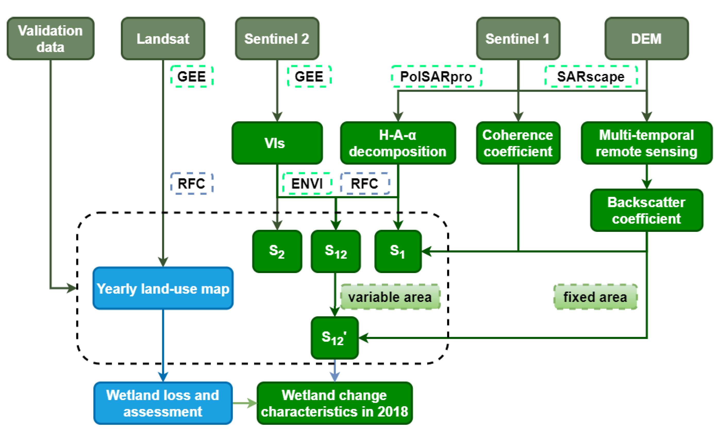
3. Methods
3.1. Yearly Land-Use Mapping in GEE
3.2. Analyzing Interannual Variation of Wetland in 2018
3.3. The Impact of Historical Wetland Change Patterns on Current Wetland Characteristics
4. Results
4.1. Yearly Land-Use Mapping in GEE
4.2. Wetland Change Characteristics in 2018
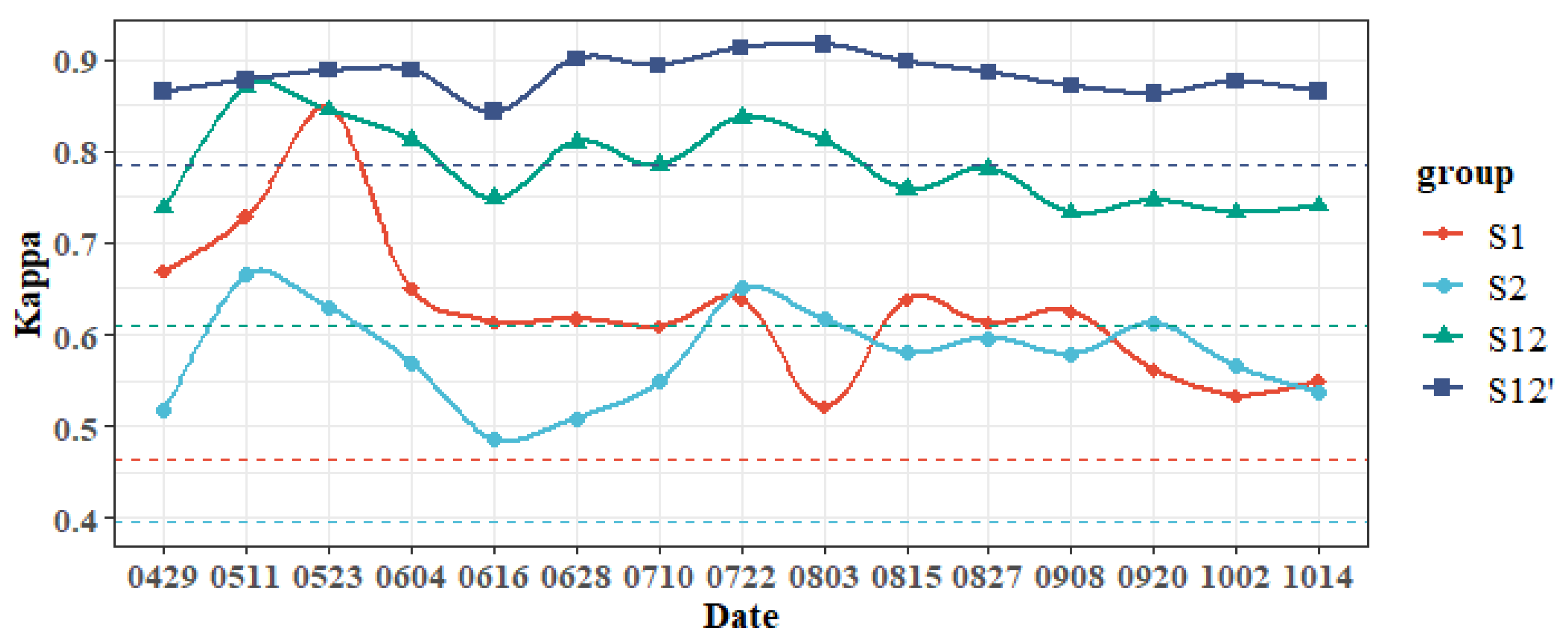
4.2.1. Twelve Days of Land-Use Mapping with Optical and SAR Data
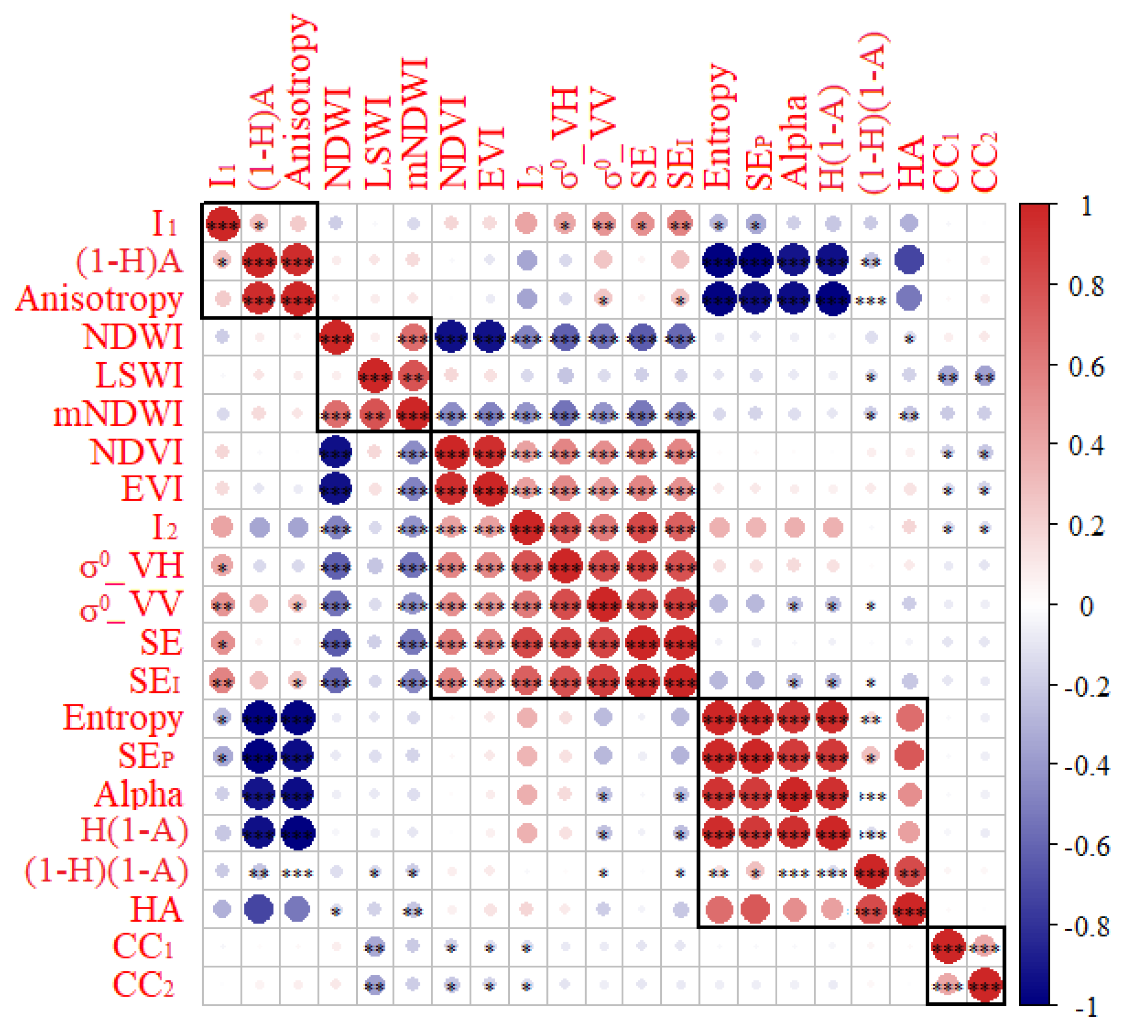
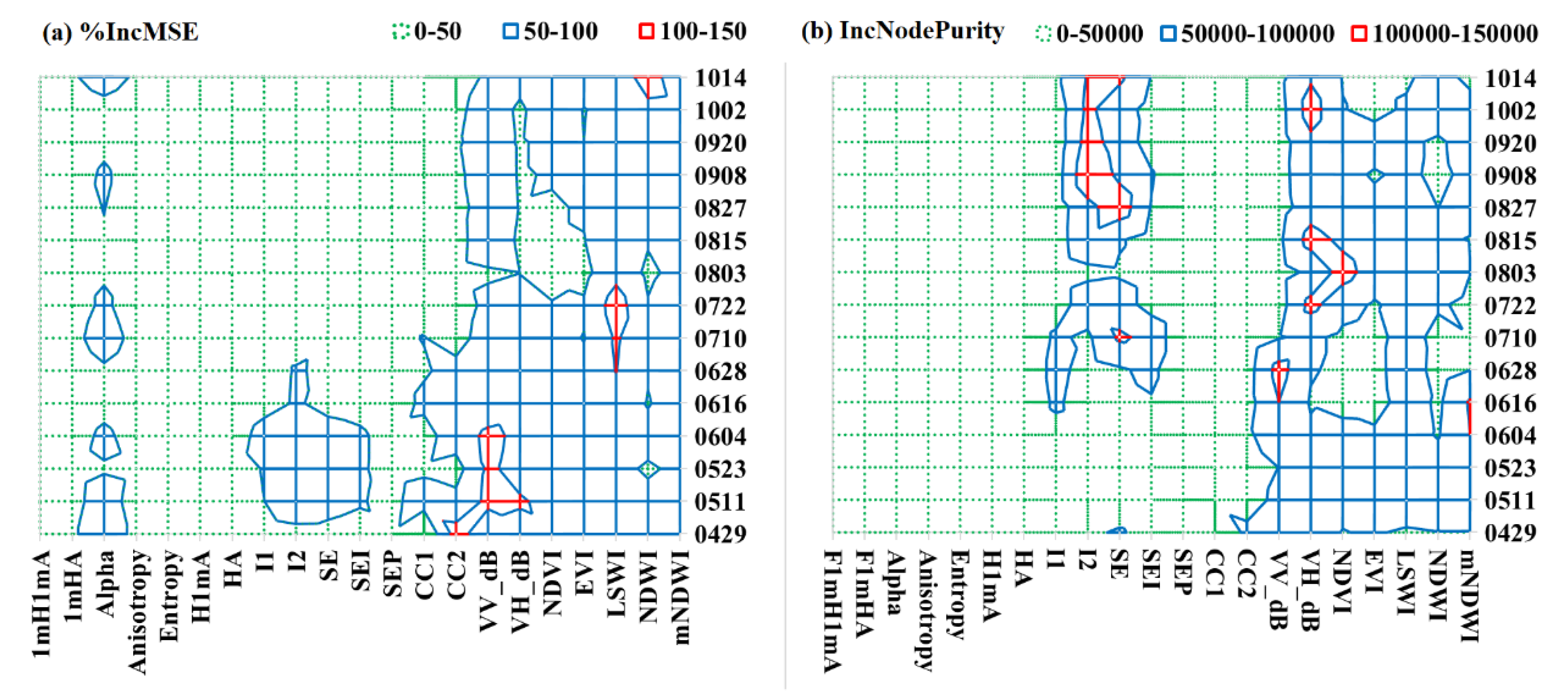
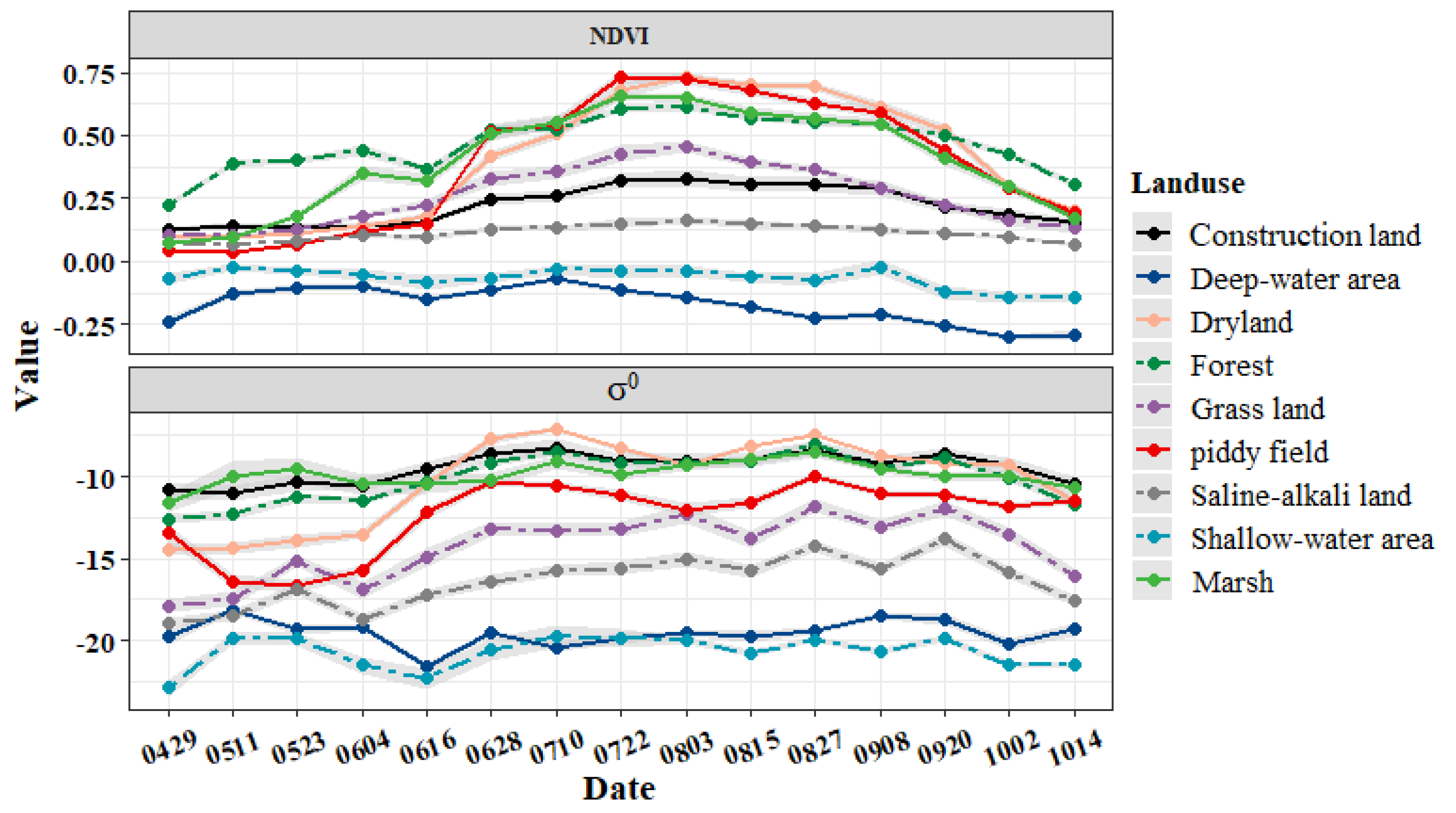
4.2.2. The Parameter Characteristics in Different Land-Use Types
4.3. The Impact of Historical Wetland Changes on Current Wetland Dynamics
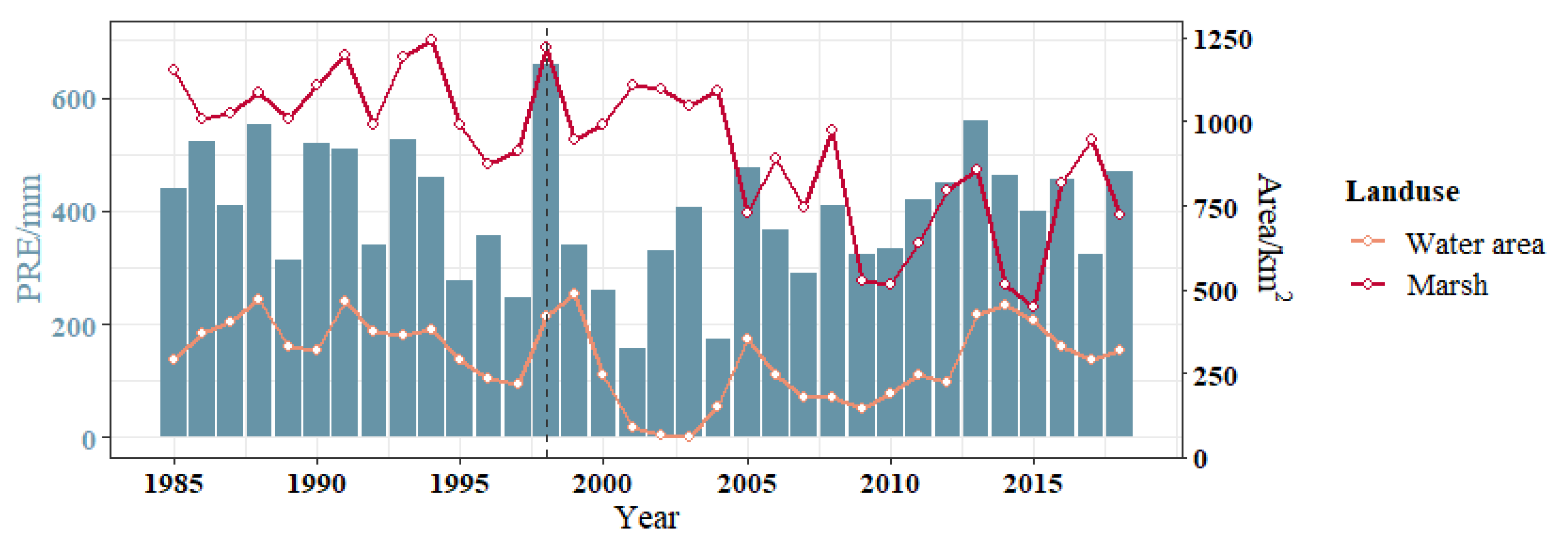
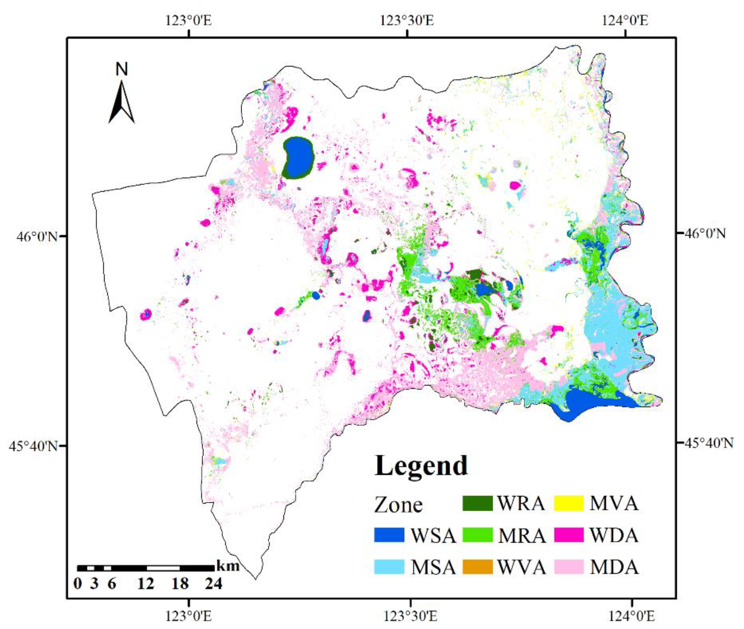
4.3.1. Wetland Loss Assessment
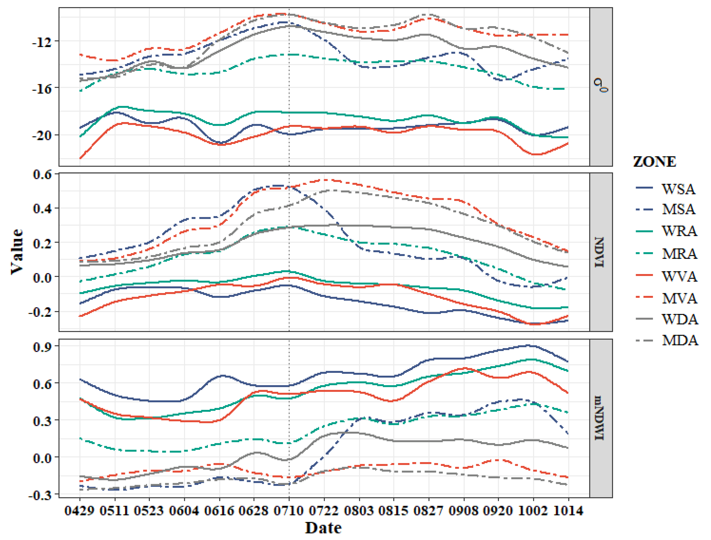
4.3.2. The Impact of Historical Wetland Changes on Current Wetland Dynamics
5. Discussion
5.1. Wetland Mapping
5.1.1. Quickly and Accurately Generating Annual Land-Use Maps in GEE
5.1.2. High Spatiotemporal Land-Use Mapping
5.2. Wetland Loss Assessment
5.3. Influences of Historic Wetland Change Characteristics on Its Current States
6. Conclusions
Supplementary Materials
Author Contributions
Funding
Data Availability Statement
Conflicts of Interest
References
- Morris, M.; Chew, C.; Reager, J.T.; Shah, R.; Zuffada, C. A novel approach to monitoring wetland dynamics using CYGNSS: Everglades case study. Remote Sens. Environ. 2019, 233, 111417. [Google Scholar] [CrossRef]
- Ogawa, H.; Male, J.W. Simulating the flood mitigation role of wetlands. J. Water Resour. Plan. Manag. 1986, 112, 114–128. [Google Scholar] [CrossRef]
- Casanova, M.T.; Brock, M.A. How do depth, duration and frequency of flooding influence the establishment of wetland plant communities? Plant Ecol. 2000, 147, 237–250. [Google Scholar] [CrossRef]
- Mitsch, W.J.; Bernal, B.; Nahlik, A.M.; Mander, Ü.; Zhang, L.; Anderson, C.J.; Brix, H. Wetlands, carbon, and climate change. Landsc. Ecol. 2013, 28, 583–597. [Google Scholar] [CrossRef]
- Davidson, N.C. How much wetland has the world lost? Long-term and recent trends in global wetland area. Mar. Freshw. Res. 2014, 65, 934–941. [Google Scholar] [CrossRef]
- Mitsch, W.J.; Hernandez, M.E. Landscape and climate change threats to wetlands of North and Central America. Aquat. Sci. 2013, 75, 133–149. [Google Scholar] [CrossRef]
- Meng, W.; He, M.; Hu, B.; Mo, X.; Li, H.; Liu, B.; Wang, Z. Status of wetlands in China: A review of extent, degradation, issues and recommendations for improvement. Ocean. Coast. Manag. 2017, 146, 50–59. [Google Scholar]
- Yin, H.; Hu, Y.; Liu, M.; Li, C.; Lv, J. Ecological and Environmental Effects of Estuarine Wetland Loss Using Keyhole and Landsat Data in Liao River Delta, China. Remote Sens. 2021, 13, 311. [Google Scholar]
- Lu, C.; Ren, C.; Wang, Z.; Zhang, B.; Man, W.; Yu, H.; Liu, M. Monitoring and Assessment of Wetland Loss and Fragmentation in the Cross-Boundary Protected Area: A Case Study of Wusuli River Basin. Remote Sens. 2019, 11, 2581. [Google Scholar]
- Hu, S.; Niu, Z.; Chen, Y.; Li, L.; Zhang, H. Global wetlands: Potential distribution, wetland loss, and status. Sci. Total. Environ. 2017, 586, 319–327. [Google Scholar] [CrossRef] [PubMed]
- Lehner, B.; Doll, P. Development and validation of a global database of lakes, reservoirs and wetlands. J. Hydrol. 2004, 296, 1–22. [Google Scholar] [CrossRef]
- Mahdianpari, M.; Granger, J.E.; Mohammadimanesh, F.; Salehi, B.; Brisco, B.; Homayouni, S.; Lang, M. Meta-Analysis of Wetland Classification Using Remote Sensing: A Systematic Review of a 40-Year Trend in North America. Remote Sens. 2020, 12, 1882. [Google Scholar] [CrossRef]
- Rebelo, L.M.; Finlayson, C.M.; Nagabhatla, N. Remote sensing and GIS for wetland inventory, mapping and change analysis. J. Environ. Manag. 2009, 90, 2144–2153. [Google Scholar] [CrossRef] [PubMed]
- Davidson, N.C.; Fluet-Chouinard, E.; Finlayson, C.M. Global extent and distribution of wetlands: Trends and issues. Mar. Freshw. Res. 2018, 69, 620–627. [Google Scholar]
- Mahdianpari, M.; Salehi, B.; Mohammadimanesh, F.; Brisco, B.; Homayouni, S.; Gill, E.; Bourgeau-Chavez, L. Big Data for a Big Country: The First Generation of Canadian Wetland Inventory Map at a Spatial Resolution of 10-m Using Sentinel-1 and Sentinel-2 Data on the Google Earth Engine Cloud Computing Platform. Can. J. Remote Sens. 2020, 46, 15–33. [Google Scholar] [CrossRef]
- Muzirafuti, A.; Barreca, G.; Crupi, A.; Faina, G.; Paltrinieri, D.; Lanza, S.; Randazzo, G. The Contribution of Multispectral Satellite Image to Shallow Water Bathymetry Mapping on the Coast of Misano Adriatico, Italy. J. Mar. Sci. Eng. 2020, 8, 126. [Google Scholar] [CrossRef] [Green Version]
- Randazzo, G.; Cascio, M.; Fontana, M.; Gregorio, F.; Lanza, S.; Muzirafuti, A. Mapping of Sicilian Pocket Beaches Land Use/Land Cover with Sentinel-2 Imagery: A Case Study of Messina Province. Land 2021, 10, 678. [Google Scholar] [CrossRef]
- Rosenqvist, A.K.E.; Finlayson, C.; Lowry, J.; Taylor, D.M. The potential of long-wavelength satellite-borne radar to support implementation of the Ramsar Wetlands Convention. Aquat. Conserv. Mar. Freshw. Ecosyst. 2007, 17, 229–244. [Google Scholar] [CrossRef]
- Yang, X.; Qin, Q.; Yésou, H.; Ledauphin, T.; Koehl, M.; Grussenmeyer, P.; Zhu, Z. Monthly estimation of the surface water extent in France at a 10-m resolution using Sentinel-2 data. Remote Sens. Environ. 2020, 244, 111803. [Google Scholar]
- Adeli, S.; Salehi, B.; Mahdianpari, M.; Quackenbush, L.J.; Brisco, B.; Tamiminia, H.; Shaw, S. Wetland Monitoring Using SAR Data: A Meta-Analysis and Comprehensive Review. Remote Sens. 2020, 12, 2190. [Google Scholar] [CrossRef]
- Huang, X.; Xie, C.; Fang, X.; Zhang, L. Combining Pixel- and Object-Based Machine Learning for Identification of Water-Body Types From Urban High-Resolution Remote-Sensing Imagery. IEEE J. Sel. Top. Appl. Earth Obs. Remote Sens. 2015, 8, 2097–2110. [Google Scholar] [CrossRef]
- Tian, H.; Li, W.; Wu, M.; Huang, N.; Li, G.; Li, X.; Niu, Z. Dynamic Monitoring of the Largest Freshwater Lake in China Using a New Water Index Derived from High Spatiotemporal Resolution Sentinel-1A Data. Remote Sens. 2017, 9, 521. [Google Scholar]
- Rodrigues, S.W.P.; Souza-Filho, P.W.M. Use of Multi-Sensor Data to Identify and Map Tropical Coastal Wetlands in the Amazon of Northern Brazil. Wetlands 2011, 31, 11–23. [Google Scholar]
- Rahman, S.; Mesev, V. Change Vector Analysis, Tasseled Cap, and NDVI-NDMI for Measuring Land Use/Cover Changes Caused by a Sudden Short-Term Severe Drought: 2011 Texas Event. Remote Sens. 2019, 11, 2217. [Google Scholar] [CrossRef] [Green Version]
- Heine, I.; Jagdhuber, T.; Itzerott, S. Classification and Monitoring of Reed Belts Using Dual-Polarimetric TerraSAR-X Time Series. Remote Sens. 2016, 8, 552. [Google Scholar]
- Wilusz, D.C.; Zaitchik, B.F.; Anderson, M.C.; Hain, C.R.; Yilmaz, M.T.; Mladenova, I.E. Monthly flooded area classification using low resolution SAR imagery in the Sudd wetland from 2007 to 2011. Remote Sens. Environ. 2017, 194, 205–218. [Google Scholar] [CrossRef]
- Gorelick, N.; Hancher, M.; Dixon, M.; Ilyushchenko, S.; Thau, D.; Moore, R. Google Earth Engine: Planetary-scale geospatial analysis for everyone. Remote Sens. Environ. 2017, 202, 18–27. [Google Scholar] [CrossRef]
- Wang, X.; Xiao, X.; Zou, Z.; Hou, L.; Qin, Y.; Dong, J.; Li, B. Mapping coastal wetlands of China using time series Landsat images in 2018 and Google Earth Engine. ISPRS J. Photogramm. Remote Sens. 2020, 163, 312–326. [Google Scholar] [CrossRef]
- Xie, S.; Liu, L.; Zhang, X.; Yang, J.; Chen, X.; Gao, Y. Automatic Land-Cover Mapping using Landsat Time-Series Data based on Google Earth Engine. Remote Sens. 2019, 11, 3023. [Google Scholar] [CrossRef] [Green Version]
- Liu, H.; Gong, P.; Wang, J.; Clinton, N.; Bai, Y.; Liang, S. Annual dynamics of global land cover and its long-term changes from 1982 to 2015. Earth Syst. Sci. Data 2020, 12, 1217–1243. [Google Scholar]
- Chen, B.; Xu, B.; Zhu, Z.; Yuan, C.; Suen, H.P.; Guo, J.; Fu, H. Stable classification with limited sample: Transferring a 30-m resolution sample set collected in 2015 to mapping 10-m resolution global land cover in 2017. Sci. Bull. 2019, 64, 370–373. [Google Scholar]
- Jiang, H.; Liu, C.; Sun, X.; Lu, J.; Zou, C.; Hou, Y.; Lu, X. Remote Sensing Reversion of Water Depths and Water Management for the Stopover Site of Siberian Cranes at Momoge, China. Wetlands 2015, 35, 369–379. [Google Scholar] [CrossRef]
- Yang, Y.; Zhang, S.; Liu, Y.; Xing, X.; de Sherbinin, A. Analyzing historical land use changes using a Historical Land Use Reconstruction Model: A case study in Zhenlai County, northeastern China. Sci. Rep. 2017, 7, 1–17. [Google Scholar]
- Yang, Y.; Zhang, S. Historical Arable Land Change in an Eco-Fragile Area: A Case Study in Zhenlai County, Northeastern China. Sustainability 2018, 10, 3940. [Google Scholar] [CrossRef] [Green Version]
- Li, B.; Hu, Y.; Chang, Y.; Liu, M.; Wang, W.; Bu, R.; Qi, L. Analysis of the factors affecting the long-term distribution changes of wetlands in the Jing-Jin-Ji region, China. Ecol. Indic. 2021, 124, 107413. [Google Scholar] [CrossRef]
- Li, L.; Su, H.; Du, Q.; Wu, T. A novel surface water index using local background information for long term and large-scale Landsat images. ISPRS J. Photogramm. Remote Sens. 2021, 172, 59–78. [Google Scholar] [CrossRef]
- Cui, G.; Liu, Y.; Tong, S. Analysis of the causes of wetland landscape patterns and hydrological connectivity changes in Momoge National Nature Reserve based on the Google Earth Engine Platform. Arab. J. Geosci. 2021, 14, 1–16. [Google Scholar] [CrossRef]
- Heumann, B.W. Satellite remote sensing of mangrove forests: Recent advances and future opportunities. Prog. Phys. Geogr. 2011, 35, 87–108. [Google Scholar]
- Chen, B.; Xiao, X.; Li, X.; Pan, L.; Doughty, R.; Ma, J.; Giri, C. A mangrove forest map of China in 2015: Analysis of time series Landsat 7/8 and Sentinel-1A imagery in Google Earth Engine cloud computing platform. ISPRS J. Photogramm. Remote Sens. 2017, 131, 104–120. [Google Scholar] [CrossRef]
- Wang, Y.; Ma, J.; Xiao, X.; Wang, X.; Dai, S.; Zhao, B. Long-Term Dynamic of Poyang Lake Surface Water: A Mapping Work Based on the Google Earth Engine Cloud Platform. Remote Sens. 2019, 11, 21. [Google Scholar]
- Hird, J.N.; DeLancey, E.R.; McDermid, G.J.; Kariyeva, J. Google Earth Engine, Open-Access Satellite Data, and Machine Learning in Support of Large-Area Probabilistic Wetland Mapping. Remote Sens. 2017, 9, 1315. [Google Scholar] [CrossRef] [Green Version]
- Asmuß, T.; Bechtold, M.; Tiemeyer, B. On the Potential of Sentinel-1 for High Resolution Monitoring of Water Table Dynamics in Grasslands on Organic Soils. Remote Sens. 2019, 11, 1659. [Google Scholar] [CrossRef] [Green Version]
- Slagter, B.; Tsendbazar, N.E.; Vollrath, A.; Reiche, J. Mapping wetland characteristics using temporally dense Sentinel-1 and Sentinel-2 data: A case study in the St. Lucia wetlands, South Africa. Int. J. Appl. Earth Obs. Geoinf. 2020, 86, 102009. [Google Scholar] [CrossRef]
- Muro, J.; Canty, M.; Conradsen, K.; Hüttich, C.; Nielsen, A.A.; Skriver, H.; Menz, G. Short-Term Change Detection in Wetlands Using Sentinel-1 Time Series. Remote Sens. 2016, 8, 795. [Google Scholar] [CrossRef] [Green Version]
- Zhang, M.; Li, Z.; Tian, B.; Zhou, J.; Tang, P. The backscattering characteristics of wetland vegetation and water-level changes detection using multi-mode SAR: A case study. Int. J. Appl. Earth Obs. Geoinf. 2016, 45, 1–13. [Google Scholar] [CrossRef]
- Ludwig, C.; Walli, A.; Schleicher, C.; Weichselbaum, J.; Riffler, M. A highly automated algorithm for wetland detection using multi-temporal optical satellite data. Remote Sens. Environ. 2019, 224, 333–351. [Google Scholar] [CrossRef]
- Rodriguez-Galiano, V.F.; Ghimire, B.; Rogan, J.; Chica-Olmo, M.; Rigol-Sanchez, J.P. An assessment of the effectiveness of a random forest classifier for land-cover classification. ISPRS J. Photogramm. Remote Sens. 2012, 67, 93–104. [Google Scholar]
- Mahdianpari, M.; Salehi, B.; Mohammadimanesh, F.; Homayouni, S.; Gill, E. The First Wetland Inventory Map of Newfoundland at a Spatial Resolution of 10 m Using Sentinel-1 and Sentinel-2 Data on the Google Earth Engine Cloud Computing Platform. Remote Sens. 2019, 11, 43. [Google Scholar] [CrossRef] [Green Version]
- Jia, M.; Wang, Z.; Mao, D.; Ren, C.; Wang, C.; Wang, Y. Rapid, robust, and automated mapping of tidal flats in China using time series Sentinel-2 images and Google Earth Engine. Remote Sens. Environ. 2021, 255, 112285. [Google Scholar] [CrossRef]
- Townshend, J.R.G.; Goff, T.E.; Tucker, C.J. Multitemporal dimensionality of images of normalized difference vegetation index at continental scales. IEEE Trans. Geosci. Remote Sens. 1985, 23, 888–895. [Google Scholar]
- Huete, A.R.; Liu, H.Q.; Batchily, K.; van Leeuwen, W. A comparison of vegetation indices global set of TM images for EOS-MODIS. Remote Sens. Environ. 1997, 59, 440–451. [Google Scholar] [CrossRef]
- Xiao, X.; Hollinger, D.; Aber, J.; Goltz, M.; Davidson, E.A.; Zhang, Q.; Moore III, B. Satellite-based modeling of gross primary production in an evergreen needleleaf forest. Remote Sens. Environ. 2004, 89, 519–534. [Google Scholar] [CrossRef]
- McFeeters, S.K. The use of the Normalized Difference Water Index (NDWI) in the delineation of open water features. Int. J. Remote Sens. 1996, 17, 1425–1432. [Google Scholar] [CrossRef]
- Xu, H. Modification of normalised difference water index (NDWI) to enhance open water features in remotely sensed imagery. Int. J. Remote Sens. 2006, 27, 3025–3033. [Google Scholar] [CrossRef]
- Bu, R.; Chang, Y.; Hu, Y.; Li, X.; He, H. Measuring spatial information changes using Kappa coefficients: A case study of the city groups in central Liaoning Province. Acta Ecol. Sinica 2005, 25, 778–784. [Google Scholar]
- Nico, G.; Pappalepore, M.; Pasquariello, G.; Refice, A.; Samarelli, S. Comparison of SAR amplitude vs. coherence flood detection methods—A GIS application. Int. J. Remote Sens. 2000, 21, 1619–1631. [Google Scholar]
- Siles, G.; Trudel, M.; Peters, D.L.; Leconte, R. Hydrological monitoring of high-latitude shallow water bodies from high-resolution space-borne D-InSAR. Remote Sens. Environ. 2020, 236, 111444. [Google Scholar] [CrossRef]
- Mohammadimanesh, F.; Salehi, B.; Mahdianpari, M.; Brisco, B.; Motagh, M. Wetland Water Level Monitoring Using Interferometric Synthetic Aperture Radar (InSAR): A Review. Can. J. Remote Sens. 2018, 44, 247–262. [Google Scholar] [CrossRef]
- Chen, Y.; Qiao, S.; Zhang, G.; Xu, Y.J.; Chen, L.; Wu, L. Investigating the potential use of Sentinel-1 data for monitoring wetland water level changes in China’s Momoge National Nature Reserve. PeerJ 2020, 8, e8616. [Google Scholar]
- Cloude, S.R.; Pottier, E. An entropy based classification scheme for land applications of polarimetric SAR. IEEE Trans. Geosci. Remote Sens. 1997, 35, 68–78. [Google Scholar] [CrossRef]
- Corcoran, J.; Knight, J.; Brisco, B.; Kaya, S.; Cull, A.; Murnaghan, K. The integration of optical, topographic, and radar data for wetland mapping in northern Minnesota. Can. J. Remote Sens. 2011, 37, 564–582. [Google Scholar] [CrossRef]
- Klouček, T.; Moravec, D.; Komárek, J.; Lagner, O.; Štych, P. Selecting appropriate variables for detecting grassland to cropland changes using high resolution satellite data. PeerJ 2018, 6, e5487. [Google Scholar]
- Tian, H.; Wu, M.; Wang, L.; Niu, Z. Mapping Early, Middle and Late Rice Extent Using Sentinel-1A and Landsat-8 Data in the Poyang Lake Plain, China. Sensors 2018, 18, 185. [Google Scholar] [CrossRef] [PubMed] [Green Version]
- Bazzi, H.; Baghdadi, N.; El Hajj, M.; Zribi, M.; Minh, D.H.T.; Ndikumana, E.; Belhouchette, H. Mapping Paddy Rice Using Sentinel-1 SAR Time Series in Camargue, France. Remote Sens. 2019, 11, 887. [Google Scholar] [CrossRef] [Green Version]
- Prigent, C.; Matthews, E.; Aires, F.; Rossow, W.B. Remote sensing of global wetland dynamics with multiple satellite data sets. Geophys. Res. Lett. 2001, 28, 4631–4634. [Google Scholar] [CrossRef] [Green Version]
- Gao, B.C. NDWI–A normalized difference water index for remote sensing of vegetation liquid water from space. Remote Sens. Environ. 1996, 58, 257–266. [Google Scholar] [CrossRef]
- Liu, R. Compositing the Minimum NDVI for MODIS Data. IEEE Trans. Geosci. Remote Sens. 2017, 55, 1396–1406. [Google Scholar] [CrossRef]
- Wang, W.; Yang, X.; Liu, G.; Zhou, H.; Ma, W.; Yu, Y.; Li, Z. Random Forest Classification Of Sediments on Exposed Intertidal Flats Using Alos-2 Quad-Polarimetric Sar Data. In Proceedings of the Xxiii Isprs Congress, Prague, Czech Republic, 2–19 July 2016; Halounova, L., Ed.; pp. 1191–1194. [Google Scholar]
- Crabbe, R.A.; Lamb, D.; Edwards, C. Discrimination of species composition types of a grazed pasture landscape using Sentinel-1 and Sentinel-2 data. Int. J. Appl. Earth Obs. Geoinf. 2020, 84, 101978. [Google Scholar] [CrossRef]
- Plank, S.; Jüssi, M.; Martinis, S.; Twele, A. Mapping of flooded vegetation by means of polarimetric Sentinel-1 and ALOS-2/PALSAR-2 imagery. Int. J. Remote Sens. 2017, 38, 3831–3850. [Google Scholar]
- Charbonneau, F.J.; Brisco, B.; Raney, R.K.; McNairn, H.; Liu, C.; Vachon, P.W.; Geldsetzer, T. Compact polarimetry overview and applications assessment. Can. J. Remote Sens. 2010, 36, S298–S315. [Google Scholar] [CrossRef]
- Lee, J.S.; Pottier, E. Polarimetric Radar Imaging: From Basics to Applications; CRC Press: Boca Raton, FL, USA, 2009; pp. 1–398. [Google Scholar]
- Mahdianpari, M.; Salehi, B.; Mohammadimanesh, F.; Motagh, M. Random forest wetland classification using ALOS-2 L-band, RADARSAT-2 C-band, and TerraSAR-X imagery. ISPRS J. Photogramm. Remote Sens. 2017, 130, 13–31. [Google Scholar]
- de Almeida Furtado, L.F.; Freire Silva, T.S.; Ledo de Moraes Novo, E.M. Dual-season and full-polarimetric C band SAR assessment for vegetation mapping in the Amazon varzea wetlands. Remote Sens. Environ. 2016, 174, 212–222. [Google Scholar] [CrossRef] [Green Version]
- Amani, M.; Salehi, B.; Mahdavi, S.; Granger, J.; Brisco, B. Wetland classification in Newfoundland and Labrador using multi-source SAR and optical data integration. GIsci. Remote Sens. 2017, 54, 779–796. [Google Scholar] [CrossRef]
- Jahncke, R.; Leblon, B.; Bush, P.; LaRocque, A. Mapping wetlands in Nova Scotia with multi-beam RADARSAT-2 Polarimetric SAR, optical satellite imagery, and Lidar data. Int. J. Appl. Earth Obs. Geoinf. 2018, 68, 139–156. [Google Scholar] [CrossRef]
- Zhang, H.; Wang, T.; Liu, M.; Jia, M.; Lin, H.; Chu, L.M.; Devlin, A.T. Potential of Combining Optical and Dual Polarimetric SAR Data for Improving Mangrove Species Discrimination Using Rotation Forest. Remote Sens. 2018, 10, 467. [Google Scholar] [CrossRef] [Green Version]
- Van Beijma, S.; Comber, A.; Lamb, A. Random forest classification of salt marsh vegetation habitats using quad-polarimetric airborne SAR, elevation and optical RS data. Remote Sens. Environ. 2014, 149, 118–129. [Google Scholar] [CrossRef]
- Yang, Y.; Liu, Y.; Xu, D.; Zhang, S. Use of Intensity Analysis to Measure Land Use Changes from 1932 to 2005 in Zhenlai County, Northeast China. Chin. Geogr. Sci. 2017, 27, 441–455. [Google Scholar] [CrossRef]
- Chen, H.; Zhang, W.; Gao, H.; Nie, N. Climate Change and Anthropogenic Impacts on Wetland and Agriculture in the Songnen and Sanjiang Plain, Northeast China. Remote Sens. 2018, 10, 356. [Google Scholar]
- Zhou, D.; Gong, H.; Wang, Y.; Khan, S.; Zhao, K. Driving Forces for the Marsh Wetland Degradation in the Honghe National Nature Reserve in Sanjiang Plain, Northeast China. Environ. Model. Assess. 2009, 14, 101–111. [Google Scholar] [CrossRef]
- Mao, D.; Luo, L.; Wang, Z.; Wilson, M.C.; Zeng, Y.; Wu, B.; Wu, J. Conversions between natural wetlands and farmland in China: A multiscale geospatial analysis. Sci. Total Environ. 2018, 634, 550–560. [Google Scholar] [CrossRef]
- Zhang, D.; Qi, Q.; Tong, S.; Wang, X.; An, Y.; Zhang, M.; Lu, X. Soil Degradation Effects on Plant Diversity and Nutrient in Tussock Meadow Wetlands. J. Soil Sci. Plant Nutr. 2019, 19, 535–544. [Google Scholar] [CrossRef]
- Zhang, D.J.; Qi, Q.; Tong, S.Z. Growth of Carex Tussocks as a Response of Flooding Depth and Tussock Patterning and Size in Temperate Sedge Wetland, Northeast China. Russ. J. Ecol. 2020, 51, 144–150. [Google Scholar] [CrossRef]
- Zhang, D.; Zhang, M.; Tong, S.; Qi, Q.; Wang, X.; Lu, X. Growth and physiological responses of Carex schmidtii to water-level fluctuation. Hydrobiologia 2020, 847, 967–981. [Google Scholar] [CrossRef]
- Zhang, D.; Tong, S.; Qi, Q.; Zhang, M.; An, Y.; Wang, X.; Lu, X. Effects of drought and re-flooding on growth and photosynthesis of Carex schmidtii Meinsh: Implication for tussock restoration. Ecol. Indic. 2019, 103, 134–144. [Google Scholar] [CrossRef]
- An, Y.; Gao, Y.; Zhang, Y.; Tong, S.; Liu, X. Early establishment of Suaeda salsa population as affected by soil moisture and salinity: Implications for pioneer species introduction in saline-sodic wetlands in Songnen Plain, China. Ecol. Indic. 2019, 107, 105654. [Google Scholar] [CrossRef]
- Wu, X.; Dong, W.; Lin, X.; Liang, Y.; Meng, Y.; Xie, W. Evolution of wetland in Honghe National Nature Reserve from the view of hydrogeology. Sci. Total Environ. 2017, 609, 1370–1380. [Google Scholar] [CrossRef] [PubMed]
- Shi, S.; Chang, Y.; Wang, G.; Li, Z.; Hu, Y.; Liu, M.; Huang, W. Planning for the wetland restoration potential based on the viability of the seed bank and the land -use change trajectory in the Sanjiang Plain of China. Sci. Total Environ. 2020, 733, 139208. [Google Scholar] [CrossRef] [PubMed]
- Yang, Y.; Zhang, S.; Wang, D.; Yang, J.; Xing, X. Spatiotemporal Changes of Farming-Pastoral Ecotone in Northern China, 1954–2005: A Case Study in Zhenlai County, Jilin Province. Sustainability 2015, 7, 1–22. [Google Scholar]
- Chen, L.; Zhang, G.; Xu, Y.J.; Chen, S.; Wu, Y.; Gao, Z.; Yu, H. Human Activities and Climate Variability Affecting Inland Water Surface Area in a High Latitude River Basin. Water 2020, 12, 382. [Google Scholar] [CrossRef] [Green Version]
- Zou, Y.; Duan, X.; Xue, Z.; Mingju, E.; Sun, M.; Lu, X.; Yu, X. Water use conflict between wetland and agriculture. J. Environ. Manag. 2018, 224, 140–146. [Google Scholar] [CrossRef]


| Evaluation Zone | Calculation |
|---|---|
| MSA (Marsh stabilization area) | SM ∩ DM ∩ RM |
| WSA (Water stabilization area) | SW ∩ DW ∩ RW |
| MDA (Marsh degradation area) | SM ∩ RO |
| WDA (Water degradation area) | SW ∩ (RO ∪ RM) |
| MRA (Marsh restoration area) | SM ∩ (RM ∪ RW)-MSA-WSA |
| WRA (Water restoration area) | SW ∩ RW-MSA-WSA |
| MVA (Marsh vulnerable area) | SM50% ∩ DM50% ∩ RM50%-MSA-WSA-MDA-WDA-MRA-WRA |
| WVA (Water vulnerable area) | SW50% ∩ DW50% ∩ RW50%-MSA-WSA-MDA-WDA-MRA-WRA |
Publisher’s Note: MDPI stays neutral with regard to jurisdictional claims in published maps and institutional affiliations. |
© 2021 by the authors. Licensee MDPI, Basel, Switzerland. This article is an open access article distributed under the terms and conditions of the Creative Commons Attribution (CC BY) license (https://creativecommons.org/licenses/by/4.0/).
Share and Cite
Shi, S.; Chang, Y.; Li, Y.; Hu, Y.; Liu, M.; Ma, J.; Xiong, Z.; Wen, D.; Li, B.; Zhang, T. Using Time Series Optical and SAR Data to Assess the Impact of Historical Wetland Change on Current Wetland in Zhenlai County, Jilin Province, China. Remote Sens. 2021, 13, 4514. https://doi.org/10.3390/rs13224514
Shi S, Chang Y, Li Y, Hu Y, Liu M, Ma J, Xiong Z, Wen D, Li B, Zhang T. Using Time Series Optical and SAR Data to Assess the Impact of Historical Wetland Change on Current Wetland in Zhenlai County, Jilin Province, China. Remote Sensing. 2021; 13(22):4514. https://doi.org/10.3390/rs13224514
Chicago/Turabian StyleShi, Sixue, Yu Chang, Yuehui Li, Yuanman Hu, Miao Liu, Jun Ma, Zaiping Xiong, Ding Wen, Binglun Li, and Tingshuang Zhang. 2021. "Using Time Series Optical and SAR Data to Assess the Impact of Historical Wetland Change on Current Wetland in Zhenlai County, Jilin Province, China" Remote Sensing 13, no. 22: 4514. https://doi.org/10.3390/rs13224514