
DP-MVS: Detail Preserving Multi-View Surface Reconstruction of Large-Scale Scenes
by
 , , , ,
Liyang Zhou
1,† ,
,
Zhuang Zhang
1,†,
Hanqing Jiang
1,†,
Han Sun
1,
Hujun Bao
2 and
Guofeng Zhang
2,* 1
SenseTime Research, Beijing 100080, China
2
State Key Lab of CAD&CG, Zhejiang University, Hangzhou 310058, China
*
Author to whom correspondence should be addressed.
†
These authors contributed equally to this work.
Remote Sens. 2021, 13(22), 4569; https://doi.org/10.3390/rs13224569
Submission received: 3 September 2021
/
Revised: 5 November 2021
/
Accepted: 8 November 2021
/
Published: 13 November 2021
(This article belongs to the Special Issue Techniques and Applications of UAV-Based Photogrammetric 3D Mapping)
Abstract
:This paper presents an accurate and robust dense 3D reconstruction system for detail preserving surface modeling of large-scale scenes from multi-view images, which we named DP-MVS. Our system performs high-quality large-scale dense reconstruction, which preserves geometric details for thin structures, especially for linear objects. Our framework begins with a sparse reconstruction carried out by an incremental Structure-from-Motion. Based on the reconstructed sparse map, a novel detail preserving PatchMatch approach is applied for depth estimation of each image view. The estimated depth maps of multiple views are then fused to a dense point cloud in a memory-efficient way, followed by a detail-aware surface meshing method to extract the final surface mesh of the captured scene. Experiments on ETH3D benchmark show that the proposed method outperforms other state-of-the-art methods on F1-score, with the running time more than 4 times faster. More experiments on large-scale photo collections demonstrate the effectiveness of the proposed framework for large-scale scene reconstruction in terms of accuracy, completeness, memory saving, and time efficiency.
1. Introduction
Multi-view stereo (MVS) reconstruction of large-scale scenes is a research topic of vital importance in computer vision and photogrammetry. With the popularization of digital cameras and unmanned aerial vehicles (UAV), it is becoming more and more convenient to capture large numbers of high resolution photos of the real scenes, which makes it more feasible to reconstruct 3D digitalized models of the scenes from the captured high-quality images. With the development of smart cities and digital twin, 3D reconstruction of large-scale scenes has attracted more attentions due to its usefulness in providing digitalized content for various applications such as urban visualization, 3D navigation, geographic mapping, and model vectorization. However, these applications usually require reconstruction of high-quality dense surface models. Specifically, 3D visualization and navigation demand realistically textured 3D surface models with complete structures and few artifacts, while geographic mapping and model vectorization depends on highly accurate dense point clouds or models with geometric details as reliable 3D priors, which are great challenges to multi-view reconstruction.
Over the past few years, significant progresses have been made in MVS, especially in the reconstruction of aerial scenes. However, most existing state-of-the-art (SOTA) methods lack sufficient details in their reconstruction results, or take huge time to achieve high reconstruction accuracy. Besides, it consumes a lot of memory to fuse high resolution depth maps to dense point cloud. Learning-based multi-view depth estimation schemes do not perform so well as traditional methods in generalization and scene detail recovery, and usually have difficulties in handling high-resolution images. In this paper, we propose a novel MVS framework for detail preserving reconstruction of dense surface model from multiple images captured by a digital camera or UAV, which we named DP-MVS. Our DP-MVS framework is designed for large-scale scene reconstruction which takes accuracy, robustness and efficiency into account, to ensure that the reconstruction is carried out in a time-and-memory-efficient way to recover accurate geometric structures with fine details. The key contributions of our system can be summarized as:
- We propose a detail preserving PatchMatch approach to ensure an accurate dense depth map estimation with geometric details for each image view.
- Considering that high resolution depth map fusion is usually memory consuming, we propose a memory-efficient depth map fusion approach for handling extremely high resolution depth map fusion, to ensure accurate point cloud reconstruction of large-scale scenes without out-of-memory issues.
- We propose a novel detail-aware Delaunay meshing to preserve fine surface details for complicated scene structures.
Experiments with quantitative and qualitative evaluations demonstrate the effectiveness and efficiency of our DP-MVS method by achieving SOTA performance on large-scale image collections captured by digital cameras or UAVs.
2. Related Work
According to the taxonomy given in [1], existing multi-view reconstruction approaches can be generally divided into four categories: voxel based methods, surface evolution based methods, feature point growing based methods, and depth-map merging based methods.
2.1. Voxel Based Methods
The voxel based methods compute a cost function on a 3D volume within a bounding box of the object. Seitz et al. [2] proposed a voxel coloring framework that identifies the voxels with high photo-consistency across multiple image views in the 3D volume space of the scene. Vogiatzis et al. [3] use graph-cut optimization to compute a photo-consistent surface that encloses the largest possible volume. These methods are limited in reconstruction accuracy and space by the voxel grid resolution. Sinha et al. [4] proposed to use photo-consistency to guide the adaptive subdivision of the 3D volume to generate a multi-resolution volumetric mesh that is densely tesselated around the possible surface, which breaks through the voxel resolution limitation to some extent. However, large-scale scenes are difficult for this method due to its high computational and memory costs. Besides, these methods are only suitable for compact objects with a tight enclosing bounding box.
2.2. Surface Evolution Based Methods
The surface evolution based methods iteratively evolve from an initial surface guess to minimize the photo-consistency measurement. Faugeras and Keriven [5] deduce a set of PDEs from a variational principle to deform an initial set of surfaces toward the objects to be detected. Hernández et al. [6] proposed a deformable model framework which fuses texture and silhouette driven forces for the final object surface evolution, based on an initial surface that should be close enough to the objective one. Hiep et al. [7] use a minimum s-t cut based global optimization to generate a initial visibility consistent mesh from dense point cloud, and then capture small geometric details with a variational mesh refinement approach. Li et al. [8] use an adaptive resolution control to classify the initial mesh into significant and insignificant regions, and accelerate the stereo refinement by culling out and simplifying most insignificant regions, while still refining and subdividing the significant regions to a SOTA level of geometry details. Romanoni and Matteucci [9] proposed a model-based camera selection method to increase the quality of pairwise camera selection, and an occlusion-aware masking to improve the model refinement robustness by avoiding the influence of occlusions on photometric error computation. A common drawback of these methods is the requirement of a reliable initial surface which is usually difficult for outdoor scenes. Cremers et al. [10] formulate multi-view reconstruction as a convex functional minimization problem that does not rely on initialization, with the exact silhouette consistency imposed as convex constraints which restrict the domain of feasible functions. However, this method uses voxel representation for reconstruction space, and is therefore unsuitable for large-scale scenes.
2.3. Feature Growing Based Methods
The feature point growing based methods first reconstruct 3D feature points from regions with textures, and then expand these feature points to textureless areas. Lhuillier et al. [11] proposed a quasi-dense approach to acquire 3D surface model, which expands the sparse feature points by resampling quasi-dense points from the quasi-dense disparity maps generated by match propagation. Goesele et al. [12] proposed a method to handle challenging Internet photo collections using per-view and per-pixel image selection for stereo matching, with a region growing process to expand the reconstructed SIFT features [13]. Based on these methods, Furukawa et al. [14] presented the SOTA MVS method called Patch-based MVS (PMVS) that first reconstructs a set of sparse matched keypoints, and then iteratively expands these keypoints till visibility constraints are invoked to filter away noisy matches. Based on PMVS, Wu et al. [15] proposed Tensor-based MVS (TMVS) for quasi-dense 3D reconstruction which combines the complementary advantages of photo-consistency, visibility and geometric consistency enforcement in MVS under a 3D tensor framework. These feature point growing methods attempt reconstructing a global 3D model using all the input images, and therefore will suffer from the scalability problem with a large number of images. Although this problem can be alleviated by dividing the input images into clusters with small overlaps like [16], its computational complexity still remains to be a problem for large-scale scenes.
2.4. Depth-Map Merging Based Methods
The depth-map merging based methods first estimate a depth map for each view and then merge all the depth maps together into a single model by taking visibility into account. Strecha et al. [17] jointly model depth and visibility as a hidden Markov Random Field (MRF), and use an EM-algorithm to alternate between estimation of visibility/depth and optimization of model parameters, without merging the depth maps to a final model. Goesele et al. [18] compute depth maps using a window-based voting approach with good matches and then merge them with volumetric integration. Merrell et al. [19] proposed a real-time 3D reconstruction pipeline, which utilizes visibility-based and confidence-based fusion for multi-view depth map fusion to online large-scale 3D model. Zach et al. [20] presented a method for range image integration by globally minimizing an energy functional consisting of a total variation (TV) regularization force and an data fidelity term. Kuhn et al. [21] use a learning-based TV prior to estimate uncertainties for depth map fusion. Liu et al. [22] produced high quality MVS reconstruction using continuous depth maps generated by variational optical flow, which requires visual hull as an initialization. However, these methods use volumetric representation for depth map fusion or rely on an initial model, and are therefore limited in scalability. Some other methods fuse the estimated depth map to point cloud, and focus on estimating confidence or uncertainty constraint to guide the depth map fusion process, which turns out to be more suitable for large-scale scenes. For example, a confidence-based MVS method in [23] developed a self-supervised deep learning method to predict the spatial confidence for multiple depth maps. Bradley et al. [24] proposed to use a robust binocular scaled-window stereo matching technique, followed by adaptive filtering of the merged point clouds, and efficient high-quality mesh generation. Campbell et al. [25] use multiple depth hypotheses with a spatial consistency constraint to extract the true depth for each pixel in a discrete MRF framework, while Schönberger et al. [26] perform MVS with pixelwise view selection for depth and normal estimation and fusion. Shen [27] computes the depth map for each image using PatchMatch, and fuses multiple depth maps by enforcing depth consistency at neighboring views, which is similar to [28], with the difference that Tola et al. used DAISY features [29] to produce depth maps. Li et al. [30] also generate depth maps using DAISY, and applied two stages of bundle adjustment to optimize the positions and normals of 3D points. However, these methods usually require complex computation for high-quality depth map estimation. To expand the reconstruction scale to a larger extent at a lower computational cost, Xue et al. [31] proposed a novel multi-view 3D dense matching method for large-scale aerial images using a divide-and-conquer scheme, and Mostegel et al. [32] innovatively proposed to prioritize the depth map computation of MVS by confidence prediction to efficiently obtain compact 3D point clouds with high quality and completeness. Wei et al. [33] proposed a novel selective joint bilateral upsampling and depth propagation strategy for high-resolution unstructured MVS. Wang et al. [34] proposed a mesh-guided MVS method with pyramid architecture, which uses the surface mesh obtained from coarse-scale images to guide the reconstruction process. However, these methods do not consider too much about how to preserve the true geometric details in depth map estimation and fusion stages. Some learning-based multi-view stereo reconstruction approaches such as [35,36,37,38,39,40] have achieved significant improvements on various benchmarks, but the robustness and generalization of these methods are still limited for natural scenes compared to the traditional methods. To better tackle practical problems such as dense reconstruction of textureless regions, some recent works try to combine learning methods with traditional MVS methods to improve generalization. For example, Yang et al. [41] use a light-weight depth refinement network to improve the noisy depths of textureless regions produced by multi-view semi-global matching (SGM). Yang and Jiang [42] combine deep learning algorithms with traditional methods to extract and match feature points from light pattern augmented images to improve a practical 3D reconstruction method for weakly textured scenes. Stathopoulou et al. [43] tackle the textureless problem by leveraging semantic priors into a PatchMatch-based MVS in order to increase confidence and better support depth and normal map estimation on weakly textured areas. However, even with these combination of traditional and learning algorithms, visual reconstruction of large textureless areas commonly present in urban scenarios of building facades or indoor scenes still remains to be a challenge. Some recent works such as [44,45] focus on novel path planning methods for the high-quality aerial 3D reconstruction of urban areas. Pepe et al. [46] apply SfM-MVS approach to airborne images captured by nadir and oblique cameras to build 2.5D map and 3D models for urban scenes. These works make efforts to improve the global reconstruction completeness and scalability for large-scale urban scenes, but pay less attention to the local reconstruction geometric details or textureless challenge.
Depth map estimation is vitally important for a high-quality MVS reconstruction. Recently, PatchMatch stereo methods [26,47,48,49,50] have shown great power in depth map estimation with their fast global search for the best matches in other images, with different kinds of propagation schemes developed or improved. For example, Schönberger et al. [26], Zheng et al. [48] both use sequential propagation scheme, while [49,51] both utilize checkerboard-based propagation to further reduce runtime. ACMM [50] extends the work of [51] by introducing a coarse-to-fine scheme for better handling textureless areas. Assuming the textureless areas are piecewise planar, ACMP [52] extends ACMM by contributing a novel multi-view matching cost aggregation which takes both photometric consistency and planar compatibility into consideration, and TAPA-MVS [53] proposed novel PatchMatch hypotheses to expand reliable depth estimates to neighboring textureless regions. Furthermore, Schönberger et al. [26], Xu and Tao [50] both use a forward/backward reprojection error as an additional error term for PatchMatch. MARMVS [54] additionally select the optimal patch scale for each pixel to reduce matching ambiguities. However, these methods focus on speeding up computation and handling textureless regions, but seldom have any strategy for geometric detail preserving, which is exactly the main focus of our method.
3. Materials and Methods
3.1. System Overview
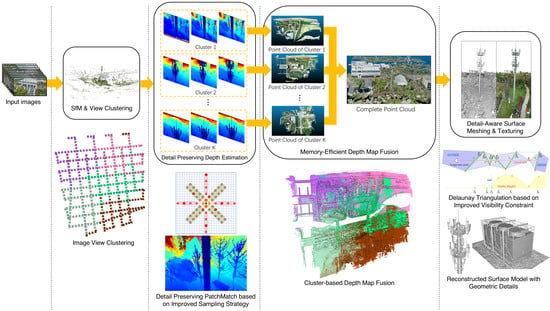
Suppose a large-scale scene is captured by multiple RGB images with digital cameras mounted on terrestrial or UAV platforms, denoted as , where N is the number of input images. Our dense 3D reconstruction system is applied for the inputed multi-view images to robustly reconstruct an accurate surface model of the captured scene. We now outline the steps of the proposed multi-view reconstruction framework, as shown in Figure 1.
Our DP-MVS framework first reconstructs a sparse map for the input multi-view images using an incremental Structure-from-Motion (SfM) framework similar to Schönberger and Frahm [55]. Then, the image views are divided into a number of clusters according to covisibility relationship based on the reconstructed sparse map. For each cluster, a novel detail preserving PatchMatch approach is applied to estimate a dense depth map for each image view i. Then, the depth maps in each cluster are fused to a noise-free dense point cloud. After that, point clouds of all the clusters are merged into a final point cloud denoted by . Finally, a detail-aware Delaunay triangulation is used to extract the final surface mesh of the captured scene from the merged point cloud, which is represented as . The main steps of our framework will be described in detail in the following subsections.
3.2. Detail Preserving Depth Map Estimation
Our method adopts a novel PatchMatch based stereo method for accurate depth map estimation with detail preservation. A well-known PatchMatch scheme is sequential propagation, which alternatively performs upward/downward propagation during odd iterations and reverse propagation during even iterations. Because only neighborhood pixels are referred during one propagation, this scheme is more sensitive to textureless regions. Furthermore, sequential propagation can only be parallelized at the row or column level, which cannot fully utilize the strength of modern multi-core GPU. Another PatchMatch scheme is checkerboard-based propagation, in which the reference image is partitioned into a checkerboard pattern of “red” and “black” pixels. Propagation and optimization is performed for all “red” pixels in odd iterations and all “black” pixels in even iterations, and is therefore more suitable for parallelized handling of high-resolution images. The standard checkerboard propagation scheme was firstly introduced by [49], which consumes a lot of time to calculate normalized cross correlation (NCC) of multiple sample points from multiple views at each single propagation. ACMM [50] improves the scheme by introducing a multi-hypothesis joint view selection strategy. The strategy is more suitable for depth estimation of planar structures, where the samples with high confidence could be propagated readily along smooth surface. However, if there is a foreground object with structure thinner than the sampling window size, the hypotheses are very likely to be sampled to the background regions, which might force the foreground depth to shift to the background position. Inspired by [26], we propose a detail preserving PatchMatch method based on the diffusion-like propagation scheme, which ensures both high accuracy and completeness of the estimated depth map, especially for accurate reconstruction of detailed structures.
Figure 2 shows the comparison results of depth estimation by ACMM and our proposed method for the experimental case “B5 Tower”, with both sampling strategies illustrated to show the difference. Take the pixel highlighted in Figure 2a as an example. Most sample points of ACMM lie in the background regions, which mistakenly wipes its depth to background level, as illustrated in Figure 2b. To better solve this problem, we change 4 V-shaped areas of ACMM to oblique long strip areas to obtain more even distribution of hypotheses. This improved sampling strategy is more favorable to the recovery of thin objects than ACMM, considering it increases the probability of sampling foreground thin object regions. In addition, we observe that the sequential-based propagation strategy is helpful to detail recovery. An important reason is that it only propagates neighboring depths and a reliable hypothesis could be spread further along horizontal and vertical directions. Inspired by this observation, we further add the four-neighboring hypotheses. Thus, there are 12 hypotheses totally, which increases the time complexity of a single propagation by half. In order to improve computational efficiency, the four-neighboring hypotheses are sorted in descending according to their NCC cost and the top-K ones are selected as the final hypotheses, with in our experiments. We exhibit the generated depth maps and normal maps of case “B5 Tower” estimated by ACMM and our strategy in Figure 2c,d. Here, we use the same multi-scale framework as ACMM for our strategy as a fair comparison. As can be seen in the red rectangles, the depth map estimated by our proposed method contains richer geometric details, with more accurate normal map, especially for thin structures. Actually, our dense matching method can reconstruct thin structures with at least 2 pixels width, the corresponding Ground Sample Distance (GSD) is cm at flying altitude of 30 m.
In the refinement step, for each pixel p of the current image view, we generate a perturbed depth and normal hypothesis by perturbing the current depth and normal estimation . A random depth and normal hypothesis is also generated denoted as . These newly generated depths and normals are combined with the current one to yield 6 additional candidate depth and normal pairs , , , , , . During each iteration, for each pixel, we choose the depth and normal estimation with the best NCC cost from the set of candidate depths and normals, to further refine its current depth and normal estimation. Usually, 3∼5 iterations are sufficient for the depth maps and normal maps to converge.
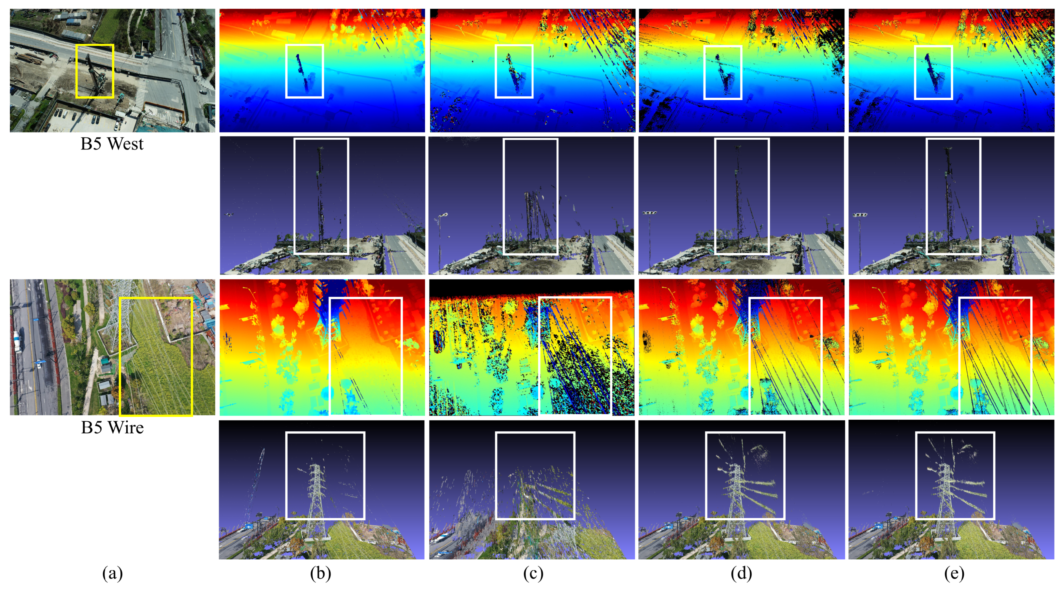
We compare our proposed scheme with SOTA methods including ACMM, OpenMVS [56] and COLMAP [26,55] in four cases “ZJU Fan”, “B5 Tower”, “B5 West” and “B5 Wire” captured by UAV with resolution . For fair comparisons, we use our SfM results as the input to these methods. Thus for COLMAP, we actually only use its MVS module [26]. We perform depth estimation by choosing 8 reference images for the current image, except OpenMVS, for which we use the default setting. The depth map results are given together with their corresponding point clouds by projecting the depth values forward to 3D space to more directly show the 3D geometry of the depth maps. As shown in the highlighted rectangle regions of the depth maps and the point clouds in Figure 3, with the proposed sampling strategy, our depth estimation method performs better than the checkerboard propagation scheme of ACMM and the sequential propagation scheme of OpenMVS and COLMAP in thin structure depth recovery. Additionally, as can be seen in Figure 3, the produced depth maps are more complete and less noisy compared with OpenMVS and COLMAP, which validates the proposed method.
3.3. Memory-Efficient Depth Map Fusion
We adopt the the graph-based framework proposed by [26] for depth map fusion, in which the consistent pixels are connected according to the geometry and depth consistency from multi-view images recursively. This method requires loading all the depth maps and normal maps into memory in advance. Therefore, for large-scale scenes of high-resolution images, out-of-memory problem will be the bottleneck. To solve this problem, we divide the scene into multiple clusters and fuse the depth maps of each cluster to an individual point cloud separately. Finally, all the clusters are merged into a complete point cloud.
Theoretically, the memory complexity of N image views with resolution is , since the main memory bottleneck is to load all the depth maps and normal maps in advance. Therefore, to avoid out-of-memory, the image views should be evenly divided into a few clusters, so that all the depth maps inside one cluster could be loaded into a single computer at once without out-of-memory risk. We adopt K-means algorithm to perform the partition. Specifically, we first estimate a cluster number K, based on the total image view number N divided by the maximum number of image views supported by each cluster denoted as n, that is:
We set for image resolution in our experiments. Then, we initialize K seed image views and iteratively classify all the other image views based on their distances to the cluster centers and covisibility scores. Therefore, for each image view , we define the distance criterion to the kth cluster for K-means as:
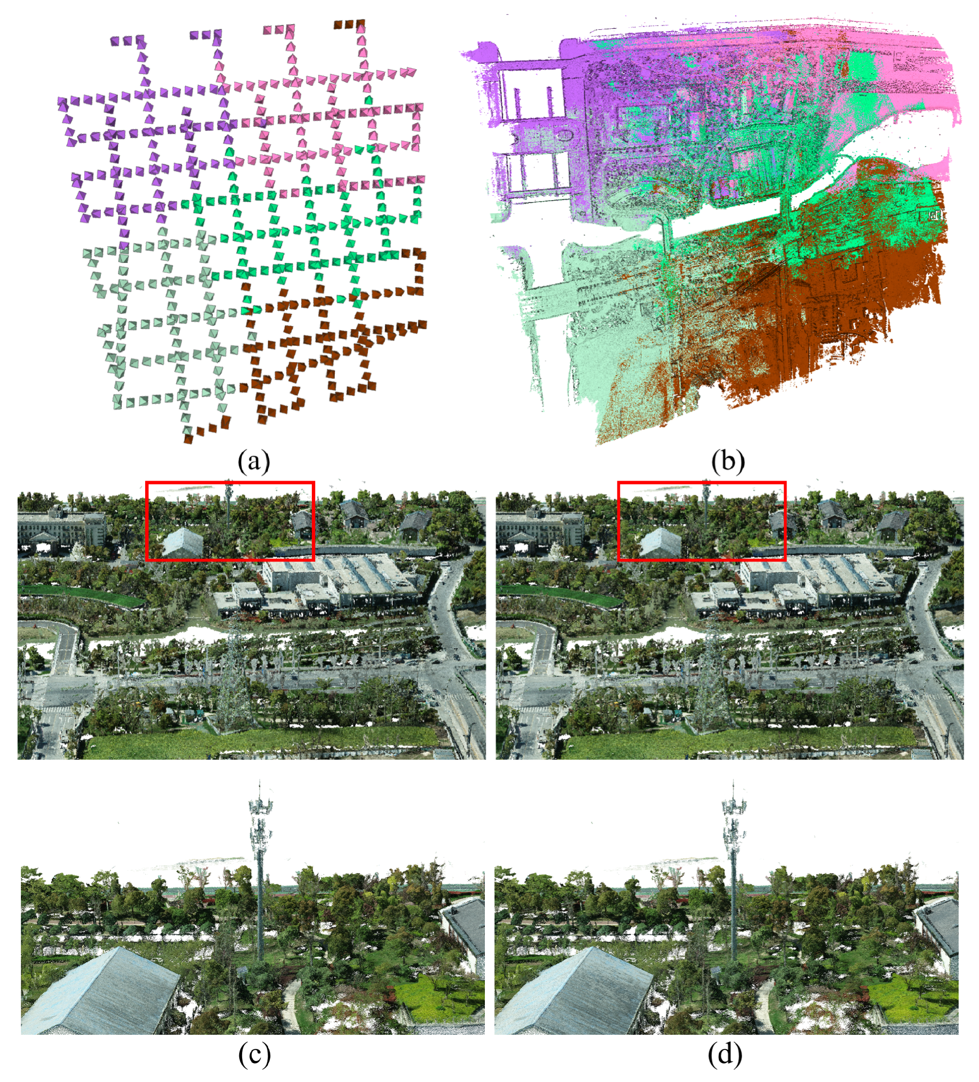
where . Here is a newly defined distance between and the kth cluster, which measures both the Euclidian distance and the covisibility between them. is the camera center of . is the barycenter of the camera centers of all the image views contained in the kth cluster. is the normalized covisibility score. is the number of SIFT feature correspondences between image views i and j, and is the set of image views in the kth cluster. Intuitively, an image view with closer distance and stronger connectivity to a cluster will be prioritized into the cluster. In order to ensure the time efficiency of fusion, the number of images contained in each cluster should be almost the same. We first choose the cluster with farthest distance to all the other clusters. If it has less than n number of views, we push image views from other clusters into it in the ascending order of until the number of views reaches n, otherwise the redundant images are popped out in the descending order of , and pushed into the cluster k with the minimal until the number of views reaches n. Meanwhile, the fused point clouds of neighboring clusters might be inconsistent at the boundary. The reason is that the partition makes the connected pixels broken into different parts, which results in a slight boundary difference from the original fused point cloud. Thus, we add additional connected images to ensure there are sufficient overlapping regions between neighboring clusters, which increases the point cloud redundancy to a certain extent. To eliminate redundancy, we merge those points from adjacent clusters if their projections on the overlapping images are the same, and the projection depth error and normal error are below certain thresholds, which are set to and respectively in the experiments. In this way, we ensure that the final point cloud is almost the same as the result without image view clustering.
We show the image view clustering result of case “B5 West” with totally 513 images of resolution and in Figure 4a,b, which runs on our server platform with 500 GB memory. We set according to Equation (1). The fused point clouds with and without image view clustering are also given in Figure 4c,d to show the effectiveness of our memory-efficient depth map fusion, which saves the memory cost from 87 GB without clustering, to 28 GB with 5 clusters for the case “B5 West”, but brings almost no difference to the quality of the final fused point cloud, with the point cloud redundancy increased only by of the total fused point cloud size.
3.4. Detail-Aware Surface Meshing
After obtaining a dense point cloud fused with multiple depth maps, we can reconstruct a surface mesh from this point cloud using Delaunay triangulation. Conventional Delaunay triangulation usually has difficulty in reconstructing geometric details such as thin structures or rough surfaces, due to its sensitivity to the noisy points that easily drones out surface details. One straightforward idea to handle thin structures is to extract 3D curves from multi-view image edges, and generate mesh from the tetrahedra topologized by both points and curves, which is used in [57]. However, since detailed structures like rough surfaces cannot be represented by curves, these methods are designed to better handle line structures specially. In this subsection, we propose a more general visibility-based Delaunay triangulation method for meshing dense point cloud, which pays more attention to the reconstruction of thin structures and rough surfaces by improving the visibility constraint to further eliminate the impact of noisy points, and using point density as a new density constraint to better preserve detailed geometry.
Each point P in the dense point cloud contains the set of image views from which it has been triangulated and visible. 3D Delaunay triangulation is applied to these points to build tetrahedra . Then, the tetrahedra are labeled inside or outside the surface through an energy minimization framework, with the labeling denoted by . We follow the previous methods [58,59] by using MRF approach to solve the tetrahedron binary labeling problem. Here, we use a graph-cuts framework similar to [58] to set up the graph of tetrahedra. Denote the directed graph as , where each node is a tetrahedron, and each edge is the triangular facet shared by two neighboring tetrahedra. For each tetrahedron , . The energy function for tetrahedron labeling problem is defined as:
where is the data term for tetrahedron , and is the smooth term for facet f which is shared by two neighboring tetrahedra . All the data terms and smooth terms are initialized to 0. As shown in Figure 5a, for each point and one of its visible image view , a line of sight shoots from the camera center of to P, and intersects with a number of facets in . For the tetrahedron that lies in, we consider it more likely to be outside the surface, and penalize its data term for case. For the tetrahedron that contains P and intersects with the extended line of sight, we consider it inside the surface, and penalize its data term for case. For each facet intersected with the line of sight, we consider it less likely to be shared by two tetrahedra with different labels, and penalize its smooth term for the case of different labels. Therefore, for each shooting of line of sight, we follow the strategies discussed above to accumulate the data terms and smooth terms as follows:
where is a constant parameter, which we set to 1 in our experiments. , and are the density weight, visibility weight and quality weight respectively. Labatut et al. [58] only use visibility weight and quality weight, which has limitation in preserving geometric details. In comparison, we propose this novel density weight to enforce the accuracy of rough surface geometry, considering the output surface should be closer to where the point cloud has denser spacing, while the sparse points are more likely to be outliers. The density weight is computed for each facet by:
where is the total edge length of f divided by the total number visible image views for vertices of f, which encourage the facet to be denser in spacing and have more sufficient visible images to be reliable. The value of is set according to the distribution of , which we set to be -order minimum of . controls the the influence of density weight, which is set to in our experiments. Affected by this weight, the surface will tend to appear in denser point regions with more visible image view supports, which is helpful to preserving rough surface details.
As in [58], visibility weight is used to penalize the visibility conflicts of dense points. Labatut et al. define the visibility weight as:
where is the distance between the intersection of f with the line of sight and the point P, which penalizes the facet far from P to appear in the final surface. However, considering that noisy points may introduce the incorrect accumulations of visibility weights along the line of sight, which might lead to the loss of thin structures. To better handle the influence of noisy points, we propose an intersection stop mechanism for smooth term accumulation. Denoting the distance between and P as , when a facet intersected with the line of sight satisfies the two conditions which are and , this facet will be the end of the intersection process, and the facets left to be intersected will be ignored. Here is the score of uncertainty of P computed in Section 3.3. In this way, the incorrect accumulation caused by noisy points will be relieved by reliable facets with sufficient visible image views and dense vertex spacing, to better reconstruct details with thin structure.
As defined in [58], the quality weight , where and are the angles between and the circumspheres of the two neighboring tetrahedra and respectively, which ensures the global surface quality by giving stronger smoothness connection between tetrahedra of better shape.
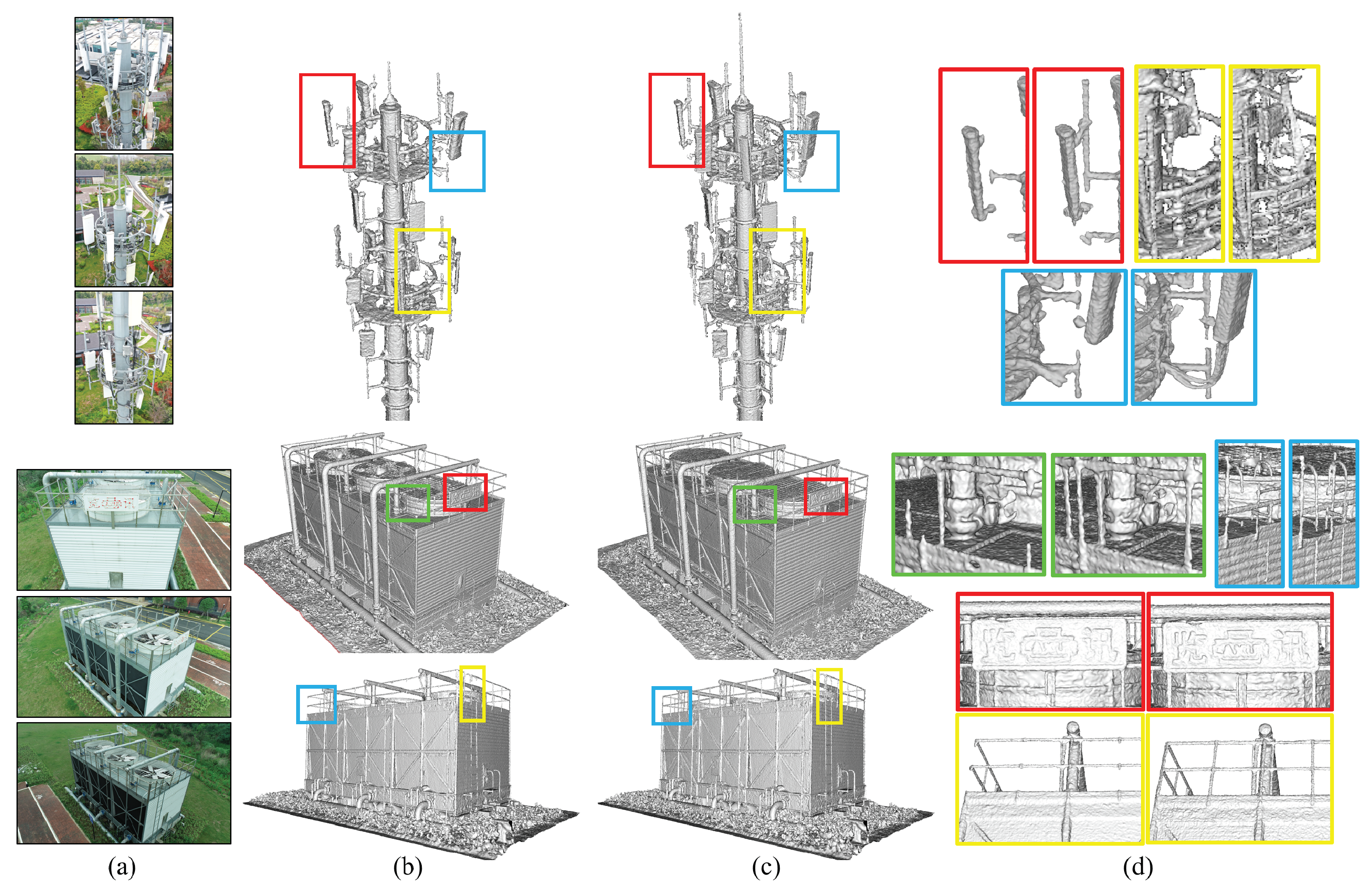
The defined energy function is finally solved by applying s-t cut on the graph to determine the binary labels, and the surface is extracted from the labeled tetrahedra by collecting the triangular facets between two neighboring tetrahedra with different labels as the final mesh surface. Experiments of cases “B5 Tower” and “ZJU Fan” in Figure 6 show that our detail-aware surface meshing approach can reconstruct more accurate surface mesh than the approach of [58], with more complete details preserved, such as the thin structures of tower antennas and fan railings, and the rough surface details of the fans, by using our improved visibility-based Delaunay triangulation.
After surface mesh of the scene being reconstructed, we can use the input multi-view images with poses to perform texture mapping for the reconstructed surface mesh. We follow the approach in [60] to perform a multi-view texture mapping to get a final textured 3D model.
4. Results
In this section, we exhibit quantitative and qualitative comparisons of our DP-MVS framework with other SOTA methods on several experimental cases. We also report the time consumption on the stages of depth estimation, fusion and meshing of different methods to show the runtime efficiency of our method. All the cases were captured by DJI PHANTOM 4 RTK UAV, except for the case “Qiaoxi Street” that was recorded by a Huawei Mate 30 mobile phone. The image resolution is for DJI PHANTOM 4 RTK and for Huawei Mate 30.
4.1. Qualitative Evaluation
We first give the qualitative comparisons of our surface reconstruction method with other SOTA methods implemented by third party source libraries including OpenMVS [56] and COLMAP [26]. For fair comparisons of surface reconstruction, we run OpenMVS and COLMAP based on our SfM input. Figure 7 shows the reconstruction results of all the methods on 5 cases “B5 West”, “B5 Tower”, “B5 Wire”, “Qiaoxi Street”, “ZJU Fan”, each of which contains some thin objects or detailed structures. For fairness to other methods, we turned off the mesh optimization process when experimenting with OpenMVS. From the experimental results we can see that our DP-MVS approach performs better than the other methods in the finally generated 3D models, especially in those regions which contain rough surface structures and thin structures, which validates the effectiveness of our DP-MVS method. As shown in the rectangle regions of Figure 7, the geometric details of the rough surface structures of the buildings, and the thin structures of the tower antennas and fan railings are better reconstructed by our detail preserving depth map estimation and detail-aware surface meshing, compared to other SOTA methods.
We also qualitatively compare our surface reconstruction method with the third party software RealityCapture v1.2 by Capturing Reality (www.capturingreality.com accessed on 3 September 2021) on the cases “ZJU Fan” and “B5 West”, as shown in Figure 8. From the reconstructed models, we can see that RealityCapture loses geometric details especially in thin structures. In comparison, our DP-MVS performs better in both reconstruction completeness and geometric details, as can be seen in the highlighted rectangle regions.
4.2. Quantitative Evaluation
Table 1 provides the quantitative comparison of our DP-MVS system with other SOTA methods on the case “ZJU CCE” which captures an academic building and a clock tower occupying an area of almost 3000 m. The ground truth (GT) 3D model of “ZJU CCE” was captured by laser scanning for accuracy evaluation on both Root Mean Squared Error (RMSE) and Mean Absolute Error (MAE). For model accuracy evaluation, we use CloudCompare (http://cloudcompare.org accessed on 3 September 2021) to compare the reconstructed meshes with GT: we align the mesh with GT using manual rough registration followed by ICP fine registration, then evaluate the mesh-point-to-GT-plane distances. This routine is achieved with CloudCompare’s built-in functions. We can see from the model accuracy evaluation in Table 1 that compared to OpenMVS and COLMAP, our DP-MVS system reconstructs the surface model of the scene with a centimeter-level accuracy, which turns out to be the best in both RMSE and MAE. Also, from the comparison of the finally reconstructed 3D models with other methods on “ZJU CCE” in Figure 9, we can see that our approach preserves better geometric details than other methods, especially for thin structures as highlighted in the rectangles.
We further evaluate our fused point clouds on the high resolution multi-view datasets of ETH3D benchmark [61]. Table 2 lists the F1-score, accuracy and completeness of the point clouds estimated by ACMM [50], OpenMVS, COLMAP and DP-MVS. ACMM obtains higher accuracy than our DP-MVS, because it performs depth map estimation with geometric consistency guidance twice and final median filter with multiple scales to suppress depth noises, but its detailed structures are also lost. OpenMVS generates point clouds with more noise and higher redundancy, resulting in lower F1-score and accuracy. COLMAP achieves higher accuracy at the cost of lower completeness by filtering the points with low confidence and large reprojection error. In comparison, our proposed system outperforms other methods in terms of F1-score and completeness because of our detail preserving depth estimation with even distribution of four-neighboring hypotheses.
4.3. Time Statistics
Table 3 gives the time consumption of the depth map estimation, fusion and meshing of our DP-MVS and other SOTA methods. The experiments are conducted on a server platform with a 14-Core Intel Xeon E5-2680 CPU, 8 GeForce 1080Ti GPUs, and 500 GB memory. It can be seen that our pipeline is the most efficient on high-resolution images, which is more than twice faster than OpenMVS and COLMAP. Note that the time consumption of our depth map fusion step is extremely more efficient because of our memory-efficient fusion strategy as mentioned in Section 3.3, which also verifies the practical usefulness of our cluster-based depth map fusion strategy for large-scale scenes with multiple high-resolution images as input, for which other SOTA works might have both time and memory limitations.
5. Discussion
Our method reconstructs 3D models with too dense faces even in the planar regions, which results in oversampled mesh topology that gives pressure to both storage and rendering. How to further optimize and simplify the reconstructed 3D models with more optimal and more compact topology is a problem worth studying in future. Besides, our DP-MVS method focuses on how to preserve detailed structures, but does not consider too much about how to preserve good surface structures for textureless regions or non-lambertian surfaces, which are as usual as detailed structures in the natural scenes. How to jointly consider and handle these problems to develop a more powerful multi-view reconstruction strategy remains to be our future work.
6. Conclusions
In this work, we propose a detail preserving large-scale scene reconstruction pipeline called DP-MVS. We first present a detail preserving multi-view stereo method to generate rich detailed structures such as thin objects in the estimated depth maps. Then, a cluster-based depth map fusion method is proposed to handle large-scale high-resolution images with limited memory. Moreover, we alter the conventional Delaunay triangulation method by imposing new visibility constraint and density constraint to extract complete detailed geometry. The effectiveness of the proposed DP-MVS method for large-scale scene reconstruction is validated in our experiments.
Author Contributions
Conceptualization, L.Z. and Z.Z.; methodology, L.Z., Z.Z. and H.J.; software, L.Z., Z.Z. and H.S.; validation, H.S.; formal analysis, G.Z.; investigation, L.Z.; resources, G.Z. and H.B.; data curation, L.Z.; writing—original draft preparation, L.Z., H.J. and G.Z.; writing—review and editing, H.J. and G.Z.; visualization, Z.Z.; supervision, G.Z. and H.B.; project administration, H.J.; funding acquisition, G.Z. and H.B. All authors have read and agreed to the published version of the manuscript.
Funding
This research was partially supported by the National Key Research and Development Program of China under Grant 2020YFF0304300, and the National Natural Science Foundation of China (No. 61822310).
Institutional Review Board Statement
Not applicable.
Informed Consent Statement
Not applicable.
Data Availability Statement
Not applicable.
Acknowledgments
The authors wish to thank Jinle Ke, Chongshan Sheng, Li Zhou and Yi Su for their kind helps in the experiments and the development of the 3D model visualization system.
Conflicts of Interest
The authors declare no conflict of interest.
References
- Seitz, S.M.; Curless, B.; Diebel, J.; Scharstein, D.; Szeliski, R. A Comparison and Evaluation of Multi-View Stereo Reconstruction Algorithms. In Proceedings of the IEEE Conference on Computer Vision and Pattern Recognition, New York, NY, USA, 17–22 June 2006; Volume 1, pp. 519–528. [Google Scholar]
- Seitz, S.M.; Dyer, C.R. Photorealistic scene reconstruction by voxel coloring. Int. J. Comput. Vis. 1999, 35, 151–173. [Google Scholar] [CrossRef]
- Vogiatzis, G.; Esteban, C.H.; Torr, P.H.; Cipolla, R. Multiview stereo via volumetric graph-cuts and occlusion robust photo-consistency. IEEE Trans. Pattern Anal. Mach. Intell. 2007, 29, 2241–2246. [Google Scholar] [CrossRef] [Green Version]
- Sinha, S.N.; Mordohai, P.; Pollefeys, M. Multi-view stereo via graph cuts on the dual of an adaptive tetrahedral mesh. In Proceedings of the IEEE International Conference on Computer Vision, Rio de Janeiro, Brazil, 14–21 October 2007; pp. 1–8. [Google Scholar]
- Faugeras, O.; Keriven, R. Variational Principles, Surface Evolution, PDE’s, Level Set Methods and the Stereo Problem. IEEE Trans. Image Process. 1998, 7, 336–344. [Google Scholar] [CrossRef] [PubMed]
- Esteban, C.H.; Schmitt, F. Silhouette and stereo fusion for 3D object modeling. Comput. Vis. Image Underst. 2004, 96, 367–392. [Google Scholar] [CrossRef] [Green Version]
- Hiep, V.H.; Keriven, R.; Labatut, P.; Pons, J.P. Towards high-resolution large-scale multi-view stereo. In Proceedings of the IEEE Conference on Computer Vision and Pattern Recognition, Miami, FL, USA, 20–25 June 2009; pp. 1430–1437. [Google Scholar]
- Li, S.; Siu, S.Y.; Fang, T.; Quan, L. Efficient multi-view surface refinement with adaptive resolution control. In Proceedings of the European Conference on Computer Vision, Amsterdam, The Netherlands, 11–14 October 2016; Springer: Cham, Switzerland, 2016; pp. 349–364. [Google Scholar]
- Romanoni, A.; Matteucci, M. Mesh-based camera pairs selection and occlusion-aware masking for mesh refinement. Pattern Recognit. Lett. 2019, 125, 364–372. [Google Scholar] [CrossRef] [Green Version]
- Cremers, D.; Kolev, K. Multiview stereo and silhouette consistency via convex functionals over convex domains. IEEE Trans. Pattern Anal. Mach. Intell. 2010, 33, 1161–1174. [Google Scholar] [CrossRef] [Green Version]
- Lhuillier, M.; Quan, L. A quasi-dense approach to surface reconstruction from uncalibrated images. IEEE Trans. Pattern Anal. Mach. Intell. 2005, 27, 418–433. [Google Scholar] [CrossRef] [PubMed] [Green Version]
- Goesele, M.; Snavely, N.; Curless, B.; Hoppe, H.; Seitz, S.M. Multi-view Stereo for Community Photo Collections. In Proceedings of the IEEE International Conference on Computer Vision, Rio de Janeiro, Brazil, 14–21 October 2007; pp. 1–8. [Google Scholar]
- Lowe, D.G. Distinctive image features from scale-invariant keypoints. Int. J. Comput. Vis. 2004, 60, 91–110. [Google Scholar] [CrossRef]
- Furukawa, Y.; Ponce, J. Accurate, dense, and robust multiview stereopsis. IEEE Trans. Pattern Anal. Mach. Intell. 2009, 32, 1362–1376. [Google Scholar] [CrossRef] [PubMed]
- Wu, T.P.; Yeung, S.K.; Jia, J.; Tang, C.K. Quasi-dense 3D reconstruction using tensor-based multiview stereo. In Proceedings of the 2010 IEEE Computer Society Conference on Computer Vision and Pattern Recognition, San Francisco, CA, USA, 13–18 June 2010; pp. 1482–1489. [Google Scholar]
- Furukawa, Y.; Curless, B.; Seitz, S.M.; Szeliski, R. Towards internet-scale multi-view stereo. In Proceedings of the 2010 IEEE Computer Society Conference on Computer Vision and Pattern Recognition, San Francisco, CA, USA, 13–18 June 2010; pp. 1434–1441. [Google Scholar]
- Strecha, C.; Fransens, R.; Van Gool, L. Combined depth and outlier estimation in multi-view stereo. In Proceedings of the IEEE Conference on Computer Vision and Pattern Recognition, New York, NY, USA, 17–22 June 2006; Volume 2, pp. 2394–2401. [Google Scholar]
- Goesele, M.; Curless, B.; Seitz, S.M. Multi-view stereo revisited. In Proceedings of the IEEE Conference on Computer Vision and Pattern Recognition, New York, NY, USA, 17–22 June 2006; Volume 2, pp. 2402–2409. [Google Scholar]
- Merrell, P.; Akbarzadeh, A.; Liang, W.; Mordohai, P.; Frahm, J.M.; Yang, R.; Nister, D.; Pollefeys, M. Real-time Visibility-Based Fusion of Depth Maps. In Proceedings of the IEEE International Conference on Computer Vision, Rio de Janeiro, Brazil, 14–21 October 2007; pp. 1–8. [Google Scholar]
- Zach, C.; Pock, T.; Bischof, H. A globally optimal algorithm for robust TV-L1 range image integration. In Proceedings of the IEEE International Conference on Computer Vision, Rio de Janeiro, Brazil, 14–21 October 2007; pp. 1–8. [Google Scholar]
- Kuhn, A.; Mayer, H.; Hirschmüller, H.; Scharstein, D. A TV prior for high-quality local multi-view stereo reconstruction. In Proceedings of the International Conference on 3D Vision, Tokyo, Japan, 8–11 December 2014; Volume 1, pp. 65–72. [Google Scholar]
- Liu, Y.; Cao, X.; Dai, Q.; Xu, W. Continuous depth estimation for multi-view stereo. In Proceedings of the IEEE Conference on Computer Vision and Pattern Recognition, Miami, FL, USA, 20–25 June 2009; pp. 2121–2128. [Google Scholar]
- Li, Z.; Zuo, W.; Wang, Z.; Zhang, L. Confidence-Based Large-Scale Dense Multi-View Stereo. IEEE Trans. Image Process. 2020, 29, 7176–7191. [Google Scholar] [CrossRef]
- Bradley, D.; Boubekeur, T.; Heidrich, W. Accurate multi-view reconstruction using robust binocular stereo and surface meshing. In Proceedings of the IEEE Conference on Computer Vision and Pattern Recognition, Anchorage, AK, USA, 23–28 June 2008; pp. 1–8. [Google Scholar]
- Campbell, N.D.; Vogiatzis, G.; Hernández, C.; Cipolla, R. Using multiple hypotheses to improve depth-maps for multi-view stereo. In Proceedings of the European Conference on Computer Vision, Marseille, France, 12–18 October 2008; Springer: Cham, Switzerland, 2008; pp. 766–779. [Google Scholar]
- Schönberger, J.L.; Zheng, E.; Pollefeys, M.; Frahm, J.M. Pixelwise View Selection for Unstructured Multi-View Stereo. In Proceedings of the European Conference on Computer Vision, Amsterdam, The Netherlands, 11–14 October 2016; Springer: Cham, Switzerland, 2016; pp. 501–518. [Google Scholar]
- Shen, S. Accurate multiple view 3D reconstruction using patch-based stereo for large-scale scenes. IEEE Trans. Image Process. 2013, 22, 1901–1914. [Google Scholar] [CrossRef]
- Tola, E.; Strecha, C.; Fua, P. Efficient large-scale multi-view stereo for ultra high-resolution image sets. Mach. Vis. Appl. 2012, 23, 903–920. [Google Scholar] [CrossRef]
- Tola, E.; Lepetit, V.; Fua, P. DAISY: An efficient dense descriptor applied to wide-baseline stereo. IEEE Trans. Pattern Anal. Mach. Intell. 2009, 32, 815–830. [Google Scholar] [CrossRef] [PubMed] [Green Version]
- Li, J.; Li, E.; Chen, Y.; Xu, L.; Zhang, Y. Bundled depth-map merging for multi-view stereo. In Proceedings of the 2010 IEEE Computer Society Conference on Computer Vision and Pattern Recognition, San Francisco, CA, USA, 13–18 June 2010; pp. 2769–2776. [Google Scholar]
- Xue, J.; Chen, X.; Hui, Y. Efficient Multi-View 3D Dense Matching for Large-Scale Aerial Images Using a Divide-and-Conquer Scheme. In Proceedings of the Chinese Automation Congress, Xi’an, China, 30 November–2 December 2018; pp. 2610–2615. [Google Scholar]
- Mostegel, C.; Fraundorfer, F.; Bischof, H. Prioritized multi-view stereo depth map generation using confidence prediction. ISPRS J. Photogramm. Remote Sens. 2018, 143, 167–180. [Google Scholar] [CrossRef] [Green Version]
- Wei, M.; Yan, Q.; Luo, F.; Song, C.; Xiao, C. Joint bilateral propagation upsampling for unstructured multi-view stereo. Vis. Comput. 2019, 35, 797–809. [Google Scholar] [CrossRef] [Green Version]
- Wang, Y.; Guan, T.; Chen, Z.; Luo, Y.; Luo, K.; Ju, L. Mesh-Guided Multi-View Stereo With Pyramid Architecture. In Proceedings of the IEEE Conference on Computer Vision and Pattern Recognition, Seattle, WA, USA, 13–19 June 2020; pp. 2039–2048. [Google Scholar]
- Yao, Y.; Luo, Z.; Li, S.; Fang, T.; Quan, L. MVSNet: Depth Inference for Unstructured Multi-view Stereo. In Proceedings of the European Conference on Computer Vision, Munich, Germany, 8–14 September 2018; pp. 767–783. [Google Scholar]
- Yao, Y.; Luo, Z.; Li, S.; Shen, T.; Fang, T.; Quan, L. Recurrent mvsnet for high-resolution multi-view stereo depth inference. In Proceedings of the IEEE Conference on Computer Vision and Pattern Recognition, Long Beach, CA, USA, 15–20 June 2019; pp. 5525–5534. [Google Scholar]
- Chen, R.; Han, S.; Xu, J.; Su, H. Point-based multi-view stereo network. In Proceedings of the IEEE International Conference on Computer Vision, Seoul, Korea, 27 October–2 November 2019; pp. 1538–1547. [Google Scholar]
- Luo, K.; Guan, T.; Ju, L.; Huang, H.; Luo, Y. P-MVSNet: Learning patch-wise matching confidence aggregation for multi-view stereo. In Proceedings of the IEEE International Conference on Computer Vision, Seoul, Korea, 27 October–2 November 2019; pp. 10452–10461. [Google Scholar]
- Gu, X.; Fan, Z.; Zhu, S.; Dai, Z.; Tan, F.; Tan, P. Cascade cost volume for high-resolution multi-view stereo and stereo matching. In Proceedings of the IEEE Conference on Computer Vision and Pattern Recognition, Seattle, WA, USA, 13–19 June 2020; pp. 2495–2504. [Google Scholar]
- Kuhn, A.; Sormann, C.; Rossi, M.; Erdler, O.; Fraundorfer, F. DeepC-MVS: Deep confidence prediction for multi-view stereo reconstruction. In Proceedings of the International Conference on 3D Vision, Fukuoka, Japan, 25–28 November 2020; pp. 404–413. [Google Scholar]
- Yang, X.; Zhou, L.; Jiang, H.; Tang, Z.; Wang, Y.; Bao, H.; Zhang, G. Mobile3DRecon: Real-time Monocular 3D Reconstruction on a Mobile Phone. IEEE Trans. Vis. Comput. Graph. 2020, 26, 3446–3456. [Google Scholar] [CrossRef] [PubMed]
- Yang, X.; Jiang, G. A Practical 3D Reconstruction Method for Weak Texture Scenes. Remote Sens. 2021, 13, 3103. [Google Scholar] [CrossRef]
- Stathopoulou, E.K.; Battisti, R.; Cernea, D.; Remondino, F.; Georgopoulos, A. Semantically Derived Geometric Constraints for MVS Reconstruction of Textureless Areas. Remote Sens. 2021, 13, 1053. [Google Scholar] [CrossRef]
- Yan, F.; Xia, E.; Li, Z.; Zhou, Z. Sampling-Based Path Planning for High-Quality Aerial 3D Reconstruction of Urban Scenes. Remote Sens. 2021, 13, 989. [Google Scholar] [CrossRef]
- Liu, Y.; Cui, R.; Xie, K.; Gong, M.; Huang, H. Aerial Path Planning for Online Real-Time Exploration and Offline High-Quality Reconstruction of Large-Scale Urban Scenes. ACM Trans. Graph. 2021, 40, 226:1–226:16. [Google Scholar]
- Pepe, M.; Fregonese, L.; Crocetto, N. Use of SfM-MVS approach to nadir and oblique images generated throught aerial cameras to build 2.5 D map and 3D models in urban areas. Geocarto Int. 2019. [Google Scholar] [CrossRef]
- Barnes, C.; Shechtman, E.; Finkelstein, A.; Goldman, D.B. PatchMatch: A randomized correspondence algorithm for structural image editing. ACM Trans. Graph. 2009, 28, 24. [Google Scholar] [CrossRef]
- Zheng, E.; Dunn, E.; Jojic, V.; Frahm, J.M. Patchmatch based joint view selection and depthmap estimation. In Proceedings of the IEEE Conference on Computer Vision and Pattern Recognition, Columbus, OH, USA, 23–28 June 2014; pp. 1510–1517. [Google Scholar]
- Galliani, S.; Lasinger, K.; Schindler, K. Massively parallel multiview stereopsis by surface normal diffusion. In Proceedings of the IEEE International Conference on Computer Vision, Santiago, Chile, 7–13 December 2015; pp. 873–881. [Google Scholar]
- Xu, Q.; Tao, W. Multi-scale geometric consistency guided multi-view stereo. In Proceedings of the IEEE Conference on Computer Vision and Pattern Recognition, Long Beach, CA, USA, 15–20 June 2019; pp. 5483–5492. [Google Scholar]
- Xu, Q.; Tao, W. Multi-view stereo with asymmetric checkerboard propagation and multi-hypothesis joint view selection. arXiv 2018, arXiv:1805.07920. [Google Scholar]
- Xu, Q.; Tao, W. Planar prior assisted patchmatch multi-view stereo. Proc. AAAI Conf. Artif. Intell. 2020, 34, 12516–12523. [Google Scholar] [CrossRef]
- Romanoni, A.; Matteucci, M. TAPA-MVS: Textureless-aware patchmatch multi-view stereo. In Proceedings of the IEEE International Conference on Computer Vision, Seoul, Korea, 27 October–2 November 2019; pp. 10413–10422. [Google Scholar]
- Xu, Z.; Liu, Y.; Shi, X.; Wang, Y.; Zheng, Y. MARMVS: Matching Ambiguity Reduced Multiple View Stereo for Efficient Large Scale Scene Reconstruction. In Proceedings of the IEEE Conference on Computer Vision and Pattern Recognition, Seattle, WA, USA, 13–19 June 2020; pp. 5981–5990. [Google Scholar]
- Schönberger, J.L.; Frahm, J.M. Structure-from-Motion Revisited. In Proceedings of the IEEE Conference on Computer Vision and Pattern Recognition, Las Vegas, NV, USA, 27–30 June 2016; pp. 4104–4113. [Google Scholar]
- Cernea, D. OpenMVS: Multi-View Stereo Reconstruction Library. Available online: https://cdcseacave.github.io/openMVS (accessed on 3 September 2021).
- Li, S.; Yao, Y.; Fang, T.; Quan, L. Reconstructing thin structures of manifold surfaces by integrating spatial curves. In Proceedings of the IEEE Conference on Computer Vision and Pattern Recognition, Salt Lake City, UT, USA, 18–23 June 2018; pp. 2887–2896. [Google Scholar]
- Labatut, P.; Pons, J.P.; Keriven, R. Robust and efficient surface reconstruction from range data. Comput. Graph. Forum 2009, 28, 2275–2290. [Google Scholar] [CrossRef] [Green Version]
- Vu, H.H.; Labatut, P.; Pons, J.P.; Keriven, R. High accuracy and visibility-consistent dense multiview stereo. IEEE Trans. Pattern Anal. Mach. Intell. 2011, 34, 889–901. [Google Scholar] [CrossRef] [PubMed]
- Waechter, M.; Moehrle, N.; Goesele, M. Let there be color! Large-scale texturing of 3D reconstructions. In Proceedings of the European Conference on Computer Vision, Zurich, Switzerland, 6–12 September 2014; pp. 836–850. [Google Scholar]
- Schops, T.; Schonberger, J.L.; Galliani, S.; Sattler, T.; Schindler, K.; Pollefeys, M.; Geiger, A. A multi-view stereo benchmark with high-resolution images and multi-camera videos. In Proceedings of the IEEE Conference on Computer Vision and Pattern Recognition, Honolulu, HI, USA, 21–26 July 2017; pp. 3260–3269. [Google Scholar]
Figure 1.
System framework of DP-MVS, which consists of six modules including SfM, image view clustering, detail preserving depth map estimation, cluster-based depth map fusion, detail-aware surface meshing, and multi-view texture mapping.
Figure 1.
System framework of DP-MVS, which consists of six modules including SfM, image view clustering, detail preserving depth map estimation, cluster-based depth map fusion, detail-aware surface meshing, and multi-view texture mapping.

Figure 2.
Illustration of our PatchMatch sampling strategy: (a) A source image view of case “B5 Tower”. (b) The ACMM [50] sampling strategy of a pixel in the red rectangle of (a), and our improved sampling strategy. (c) The estimated depth map and normal map by ACMM. (d) Our estimated depth map and normal map, which contain better details highlighted in the red and yellow rectangles.

Figure 3.
(a) A source image view for each case of “ZJU Fan”, “B5 Tower”, “B5 West” and “B5 Wire”. (b) The depth map results of ACMM [50] and their corresponding point clouds by projecting the depths forward to 3D space. (c) The depth maps and point clouds of OpenMVS [56]. (d) The depth maps and point clouds of COLMAP [26]. (e) Our results of depth maps and point clouds, which turn out to be the best in both details and noisylessness.


Figure 4.
(a) Camera views of case “B5 West” divided into 5 clusters. (b) The final fused point cloud with points from different clusters visualized in different colors. (c) The fused point cloud without clustering. (d) The clustering-based point cloud fusion, with magnified rectangle regions to show almost no difference from (c).

Figure 5.
Illustration of our visibility weight strategy: (a) A line of sight from the camera center of an image view traverses a sequence of tetrahedra to a 3D point to accumulate the visibility weighted smooth terms. (b) The visibility weights proposed by [58]. (c) The visibility weights by our strategy, which are stopped by the end facet.

Figure 6.
(a) Three representative image views for each case of “B5 Tower” and “ZJU Fan”. (b) The reconstructed surface models of the two cases by [58]. (c) The surface models generated by our meshing approach. (d) Comparisons of the details in the rectangles of (b,c), which shows the effectiveness of our detail-aware surface meshing.

Figure 7.
Comparison of our DP-MVS pipeline with other SOTA methods on 5 cases: “B5 Tower”, “B5 West”, “Qiaoxi Street”, “ZJU Fan” and “B5 Wire”. (a) Some representative source images of each case. (b) The reconstructed surface models of OpenMVS [56]. (c) The reconstruction results of COLMAP [26]. (d) The reconstructed 3D models by our DP-MVS. Some detailed structures are highlighted in the rectangles to show the effectiveness of our reconstruction pipeline.

Figure 8.
Comparison of our method with the third party software RealityCapture, on the cases “ZJU Fan” and “B5 West”. (a) Some representative source images of each case. (b) The reconstructed 3D models using RealityCapture. (c) The reconstructed 3D models by our DP-MVS. Some detailed structures are highlighted in the rectangles to show the effectiveness of our proposed method.

Figure 9.
Comparison of our method with other SOTA methods on the case “ZJU CCE”, whose true 3D model is captured by a 3D laser scanner as GT. (a) Some representative source images. (b) The GT model captured by the 3D laser scanner. (c) The reconstructed surface model of OpenMVS [56]. (d) The reconstruction result of COLMAP [26]. (e) The reconstructed 3D model by our DP-MVS. Some detailed structures are highlighted in the rectangles to show the effectiveness of our reconstruction method.


Table 1.
The Root Mean Squared Error (RMSE) and Mean Absolute Error (MAE) of the reconstruction results by our system, OpenMVS [56] and COLMAP [26] on the case “ZJU CCE”, whose GT model is used as reference for error computation. We use bold format to highlight the smallest errors among all the methods.
| Case | Measures [cm] | OpenMVS | COLMAP | DP-MVS |
|---|---|---|---|---|
| ZJU CCE | RMSE/MAE | 4.337/2.084 | 4.476/2.275 | 3.698/1.859 |
Table 2.
Evaluation on high resolution multi-view datasets of ETH3D benchmark. It shows F1-score, accuracy and completeness at different error levels (2 cm and 10 cm), with bold format highlighting the best evaluation among all the methods including ACMM [50], OpenMVS [56], COLMAP [26] and DP-MVS.
| Dataset | Error | Measure | ACMM | OpenMVS | COLMAP | DP-MVS |
|---|---|---|---|---|---|---|
| Training dataset | 2 cm | F1-score | 78.86 | 76.15 | 67.66 | 80.11 |
| accuracy | 90.67 | 78.44 | 91.85 | 83.56 | ||
| completeness | 70.42 | 74.92 | 55.13 | 77.56 | ||
| 10 cm | F1-score | 91.70 | 92.51 | 87.61 | 94.77 | |
| accuracy | 98.12 | 95.75 | 98.75 | 95.95 | ||
| completeness | 86.40 | 89.84 | 79.47 | 93.72 | ||
| Test dataset | 2 cm | F1-score | 80.78 | 79.77 | 73.01 | 83.11 |
| accuracy | 90.65 | 81.98 | 91.97 | 84.05 | ||
| completeness | 74.34 | 78.54 | 62.98 | 82.73 | ||
| 10 cm | F1-score | 92.96 | 92.86 | 90.40 | 95.68 | |
| accuracy | 98.05 | 95.48 | 98.25 | 95.55 | ||
| completeness | 88.77 | 90.75 | 84.54 | 95.85 |
Table 3.
We report detailed time consumptions of our DP-MVS system and other SOTA methods including OpenMVS [56] and COLMAP [26] in all the steps of cases “B5 Tower”, “B5 West”, “Qiaoxi Street” and “B5 Wire”. All the time consumptions are calculated by minutes, with bold format highlighting the fastest time of all the methods.
| Case | #Images | Stages | OpenMVS | COLMAP | DP-MVS |
|---|---|---|---|---|---|
| B5 Tower | 1163 | Depth Estimation | 757.57 | 135.795 | 54.207 |
| Fusion | 99.55 | 1810.244 | 48.139 | ||
| Meshing | 132.65 | 125.49 | 158.803 | ||
| Total | 989.77 | 2071.529 | 261.149 | ||
| B5 West | 513 | Depth Estimation | 312.56 | 148.484 | 26.833 |
| Fusion | 47.53 | 214.713 | 8.413 | ||
| Meshing | 163.62 | 64.92 | 63.191 | ||
| Total | 523.71 | 428.117 | 98.437 | ||
| Qiaoxi Street | 305 | Depth Estimation | 168.87 | 69.313 | 11.318 |
| Fusion | 18.33 | 42.538 | 3.862 | ||
| Meshing | 156 | 54.1 | 56.227 | ||
| Total | 343.2 | 165.951 | 71.407 | ||
| B5 Wire | 1251 | Depth Estimation | 728.58 | 224.183 | 40.826 |
| Fusion | 99.57 | 1168.048 | 56.312 | ||
| Meshing | 220.62 | 165.4 | 130.764 | ||
| Total | 1048.77 | 1557.631 | 227.902 |
Publisher’s Note: MDPI stays neutral with regard to jurisdictional claims in published maps and institutional affiliations. |
© 2021 by the authors. Licensee MDPI, Basel, Switzerland. This article is an open access article distributed under the terms and conditions of the Creative Commons Attribution (CC BY) license (https://creativecommons.org/licenses/by/4.0/).
Share and Cite
MDPI and ACS Style
Zhou, L.; Zhang, Z.; Jiang, H.; Sun, H.; Bao, H.; Zhang, G. DP-MVS: Detail Preserving Multi-View Surface Reconstruction of Large-Scale Scenes. Remote Sens. 2021, 13, 4569. https://doi.org/10.3390/rs13224569
AMA Style
Zhou L, Zhang Z, Jiang H, Sun H, Bao H, Zhang G. DP-MVS: Detail Preserving Multi-View Surface Reconstruction of Large-Scale Scenes. Remote Sensing. 2021; 13(22):4569. https://doi.org/10.3390/rs13224569
Chicago/Turabian StyleZhou, Liyang, Zhuang Zhang, Hanqing Jiang, Han Sun, Hujun Bao, and Guofeng Zhang. 2021. "DP-MVS: Detail Preserving Multi-View Surface Reconstruction of Large-Scale Scenes" Remote Sensing 13, no. 22: 4569. https://doi.org/10.3390/rs13224569
Note that from the first issue of 2016, this journal uses article numbers instead of page numbers. See further details here.