Article

Reproduction of the Marine Debris Distribution in the Seto Inland Sea Immediately after the July 2018 Heavy Rains in Western Japan Using Multidate Landsat-8 Data

Graduate School of Advanced Science and Engineering, Hiroshima University, Higashi-Hiroshima 739-8527, Japan
*
Author to whom correspondence should be addressed.
Remote Sens. 2021, 13(24), 5048; https://doi.org/10.3390/rs13245048
Submission received: 19 November 2021 / Revised: 8 December 2021 / Accepted: 8 December 2021 / Published: 12 December 2021

Abstract

:
Understanding the spatiotemporal environment of the ocean after a heavy rain disaster is critical for satellite remote sensing research and disaster prevention. We attempted to reproduce changes in marine debris distributions using multidate data of Landsat-8 spectral reflectance acquired immediately after a heavy rain disaster in western Japan in July 2018. Data from cleaning ships were used for screening the marine debris area. As most of the target marine debris consisted of plant fragments, a method based on the corrected floating algae index (cFAI) was applied to Landsat-8 data. Data from cleaning ships clarify that most of the marine debris accumulated in the waters in the northern part of Aki Nada, a part of the Seto Inland Sea. The spectral characteristics of the corresponding marine debris spectral reflectance obtained from the Landsat-8 data were explained by the FAI with band 5 (central wavelength: 865 nm) as the maximum value. Unlike traditional FAI, cFAI eliminated the effect of background water turbidity. The Otsu method was effective for the automatic threshold determination for cFAI. Although Landsat-8 data have limited spatial resolution and observation frequency, these data were useful for understanding marine debris distribution after a heavy rain disaster.

1. Introduction

In 2018, the western part of Japan experienced a torrential rain disaster (28 June to 8 July 2018, and heavy rain in July 2018) that caused more than 200 deaths [1,2]. Because of the heavy rain, much sediment flowed from large and small rivers into the Seto Inland Sea adjacent to the affected area. The heavy sediment inflow destroyed the special oyster farming raft and created excessive marine debris (mainly derived from plants such as driftwood and plant fragments). The official marine debris collection completed by the Ministry of Land, Infrastructure, Transport, and Tourism in the Seto Inland Sea off Hiroshima Prefecture took more than a month (7 July to 17 August 2018). Marine debris poses a significant obstacle to the fishing industry. Collecting the debris took a long time, mainly because it was difficult to locate due to the area’s complicated topography and influence of ocean currents. Although more than 3 years have passed since this disaster, the distribution of marine debris at that time remains unknown. In addition, it is very important to establish a method for obtaining information about marine debris immediately after a disaster given the torrential rains that have become frequent in recent years.
To grasp the distribution of marine debris, buoys with global positioning system (GPS) equipment, aerial photographs [3,4], and numerical simulation methods [5,6] used for exploring plastic waste can be considered. However, emergency observation during heavy rains is not easy, and the flow of the Seto Inland Sea is complex. It is not always possible to reproduce the position of marine debris. Therefore, the locations of marine debris can be identified by satellites that observe the Earth periodically. Examples of exploration of suspended matter in water using satellites include the detection of farming rafts using synthetic aperture radar data [7,8] and the use of visible–near infrared data such as Terra/Aqua MODIS and Landsat-8 Operational Land Images (OLI) products for detecting floating algae using an external sensor [9,10]. Satellite remote sensing is further used to detect marine litter windrows for managing ocean plastic pollution [11]. In recent years, a scientific method for collecting word-of-mouth information using social network systems (SNS) or Internet information [12,13] has also attracted attention.
The floating algae index (FAI) algorithm is used to detect floating algae by employing conventional satellite remote sensing (RS). It realizes vegetation detection in a manner different from the method based on the normalized difference vegetation index (NDVI) by removing the influence of the seawater color in the background. In addition, a limitation of the traditional FAI algorithm [9] is that it erroneously recognizes floating plants and turbid water in water areas that are strongly affected by turbidity. The influence of turbidity in the sea is strong after a heavy rain disaster; hence, such misrecognition is considered likely when using the conventional FAI algorithm. Recently, Garcia et al. [14] were able to remove the influence of background water. Hu et al. [15] devised a new algorithm that improved detection performance in water areas affected by turbidity, and named this algorithm corrected FAI (cFAI). However, these algorithms are used to detect large living aquatic plants, and it is unknown whether they can be applied to detecting plant-derived disaster waste such as driftwood and plant pieces. Furthermore, the threshold for extracting suspended solids from cFAI is still mostly determined by a trial-and-error method. Hence, the results differ depending on the analyst.
With the aforementioned research in mind, this study aims to reproduce the actual conditions of the marine debris distribution in the Seto Inland Sea off the coast of Hiroshima Prefecture after the heavy rain in July 2018. The data used for this purpose were the marine debris information acquired by cleaning boats and satellite images. First, information on the location and amount of marine debris was collected. This information, which was published on the Internet by public institutions on an irregular basis, was mapped and graphed. Next, by applying the cFAI algorithm and objective binarization method to Landsat-8 data with a resolution of 30 m, plant-derived suspended matter (called marine debris in this study) is detected. The marine debris distribution map created using satellite data in this work is expected to aid the agency that manages the Seto Inland Sea in collecting marine debris immediately after a heavy rain disaster.

2. Materials and Methods

2.1. Study Area and Landsat-8 Data

As shown in Figure 1, the Seto Inland Sea is the largest inland sea in Japan. It is located in western Japan. The total length of the coastline is 500 km, and the average water depth is 30 m. More than 600 islands are located in this sea [16]. This inland sea has a complex structure in which a wide part called Nada is connected by a narrow waterway called Seto. Furthermore, the Seto Inland Sea has a large tidal range that exceeds 2 m around the innermost part of Nada. Hence, the tidal current in this sea is extremely strong, and there are many areas with rapid water flow at speeds of 1 m/s or more [16,17]. This study focuses on the central waters of the Seto Inland Sea off the coast of Hiroshima Prefecture, where the heavy rains in July 2018 resulted in many casualties.
According to the observation data of the Japan Meteorological Agency, the total rainfall from 0:00 on 28 June to 9:00 on 8 July exceeded 500 mm in the Chugoku region, including the Hiroshima Prefecture [18]. In particular, Higashi-Hiroshima City, Hiroshima Prefecture, experienced torrential rain of 426.5 mm in 48 h until 8:40 a.m. on July 7. Because of this heavy rain, the major inflow rivers, such as the Ota River (point ① in Figure 1) and Ashida River (point ②), and small- and medium-sized rivers, such as Kurose River (point ③) and Nuta River (point ④), in Hiroshima Prefecture carried a large amount of sediment and disaster waste, such as plant species, to the sea.
Landsat-8 data are available for the Seto Inland Sea off Hiroshima Prefecture, which is the research area, where two satellite orbits (Path 111 and Path 112) overlap as shown in Figure 1. Therefore, although the Landsat-8 data usually have a 16-day cycle, this overlap made it possible to obtain data with few clouds in a cycle of 7–9 days after the disaster. The Landsat-8 data used in the present study were the “Collection 2 Surface Reflectance” product of the OLI sensor distributed by the USGS Earth Explorer. This product is “atmospheric-corrected reflectance data” in which the effects of atmospheric gases, aerosols, and water vapor are removed. The downloaded Landsat-8 data were stored as 16-bit unsigned digital values (DN: digital number) and converted to ground surface reflectance (Rreal) using the following equation.
R real ( i ) = DN ( i ) × MULT ( i ) + ADD ( i )
where i is the Landsat-8 level-2 band (Table 1) and MULT and ADD are the reflectance conversion coefficients stored in the Landsat-8 level-2 data metadata file. The values of MULT and ADD are 2.75 × 10⁻⁵ and −2, respectively, for all bands. In this study, in addition to the four images from 9 July, 16 July, 25 July, and 1 August immediately after the heavy rain, one image of the freshwater state before the heavy rain (acquired on 20 April) was used for cFAI processing as described later.

2.2. Spectral Reflectance Data of Marine Debris

Almost no objective data other than satellite images are available to prove that large amounts of marine debris flowed into the Seto Inland Sea. In addition, during the studied heavy rainfall period, many of the roads to the port were cut off, and marine debris was scattered even at sea, making it impossible to verify the debris distribution even by a research vessel in the sea immediately after the heavy rain. Therefore, in this study, we collected data on the approximate position and amount of debris collected by marine environment maintenance vessels (referred to as cleaning ships in this study) owned by the Chugoku Regional Development Bureau of the Ministry of Land, Infrastructure, Transport, and Tourism. These data were published on the website of the Chugoku Regional Development Bureau. Table 2 lists the published materials on the status of marine debris collection. The authors created a compact map of the approximate location of marine debris by accumulating information from these published materials. In addition, the amount of marine debris collected was summarized as the time-series data of the debris accumulated every week.
To understand the basic spectral characteristics of coastal garbage in Hiroshima Prefecture, samples of driftwood, polyvinyl chloride (PVC), plastic bottles (polyethylene terephthalate, or PET), and sand were acquired from Bayside Beach Saka (★ in Figure 1) in Mizushiri, Saka-cho, Aki-gun, Hiroshima Prefecture, on 4 May 2018. Note that although we collected spectral data of those materials in our study area, multiple spectral datasets of various material including plastics are now available online [19,20]. The spectrometer used was FieldSpec4 (ASD Inc., Falls Church, VA, USA, spectral range: 350–2500 nm; spectral resolution: 3 nm at 700 nm and 8 nm at 1400 and 2100 nm), and the radiance of objects was measured vertically downward. The reflectance of each object was derived from the radiance ratio of the white reference plate (SRT-99-050 from Labsphere, Inc., North Sutton, NH, USA) and the object.

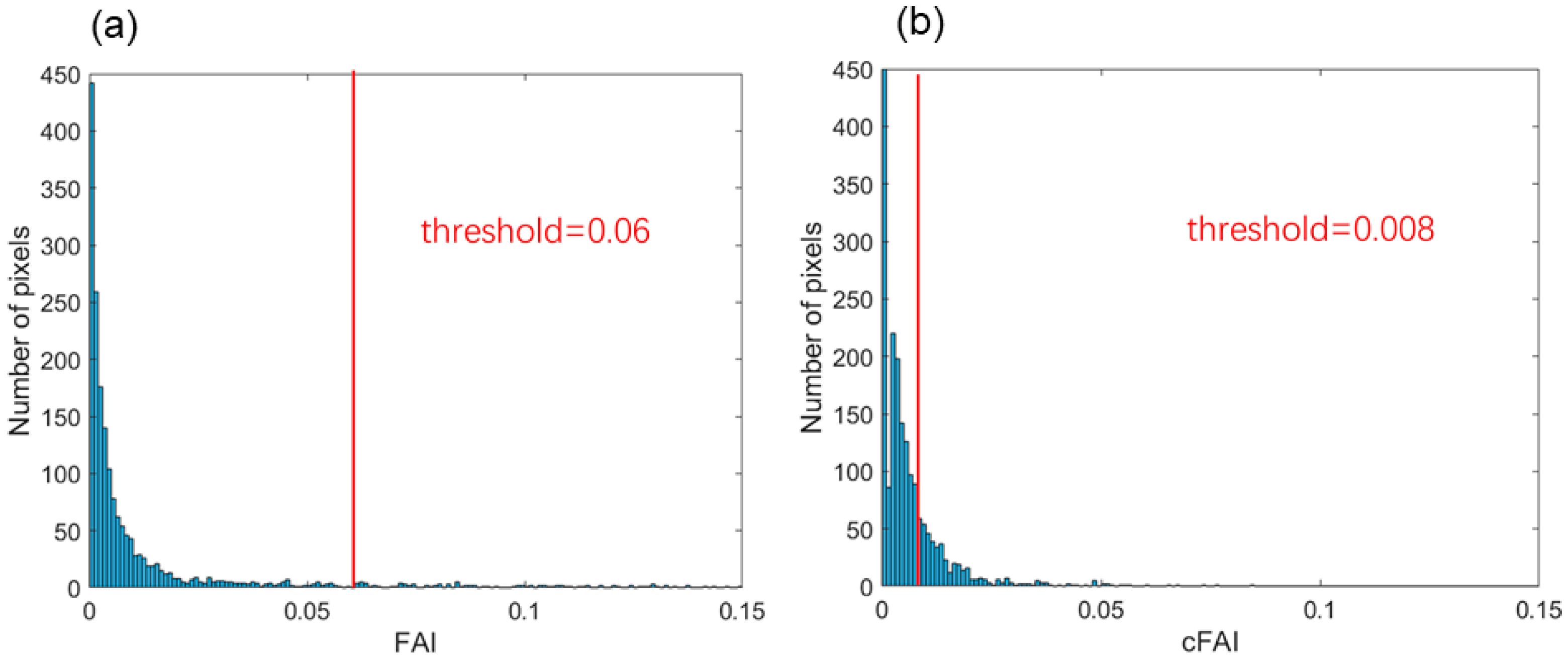
2.3. Extraction of Marine Debris from Satellite Data

In this study, to detect plant-derived marine debris, we first calculated FAI using Hu’s equation [9]:
FAI = R r c ( NIR ) R r c ( NIR )
R r c ( NIR ) = R r c ( RED ) + ( R r c ( SWIR ) R r c ( RED ) ) ( λ NIR λ RED ) ( λ SWIR λ RED )
where Rrc is the Rayleigh-corrected reflectance; however, in this study, the level-2 aerosol-corrected reflectance was used instead of the Rayleigh-corrected one. RED indicates red (OLI Band 4); NIR indicates near-infrared (OLI Band 5); SWIR indicates mid-infrared (OLI Band 6); and λ indicates wavelength. This formula is based on the fact that the high NIR reflectance (A) of a plant-derived substance and the slope of the reflectance of background water with the same wavelength as the baseline (B) formed by the NIR and SWIR reflectances are almost equal. We assumed that A–B can be used as an index of marine debris.
However, this assumption may not hold in the case of turbid background water, as is seen after heavy rain. To solve this problem, we used the method proposed by Hu et al. [15]. For the MODIS-derived FAI image of the Yellow Sea, Hu et al. [15] determined the FAI of background seawater (FAIsw) using two criteria and successfully detected drifting algae while suppressing false detection due to turbid water. Our FAI calculation performed according to the method of Hu et al. [15] is briefly described below.
For the first criterion, we calculated the difference between the gradient of the FAI image and the gradient of the Rrc (RED) image for each pixel (this difference is hereinafter referred to as the corrected gradient of FAI (cGFAI)) Subsequently, we considered the pixels with cGFAI below a certain threshold (TcG) as pixels of seawater without marine debris. For the gradient of FAI and Rrc (RED) images, the following equation given by Hu et al. [15] was used:
y i = 1 8 j = 1 8 ( y i y j x i , j ) 2 ,   j i ,
where ∇yi is the magnitude of the gradient of the ith pixel of the image y (for example, FAI); yj is the FAI value of the eight pixels adjecent to the ith pixel; and xi,j is the distance between the ith pixel and the eight adjacent pixels (i.e., 1 or 1.414 times the spatial resolution). The threshold TcG is the maximum cGFAI for the seawater that does not contain algae or marine debris. Hu et al. [15] calculated cGFAI for long-term data from several months without drifting algae and determined TcG as the long-term cGFAI with a cumulative frequency of 0.99 in all calculated frequency distributions. However, in this study, we could not obtain multiple good-quality Lansat-8 data from before the disaster. Hence, we calculated TcG using a Landsat image from 20 April 2018, which had the best image quality among images whose obtained dates are close to the heavy rain event. For the second criterion, we calculated the mean and standard deviation of the FAI in a 15 × 15 pixel kernel centered on the pixel of interest. If the FAI of the pixel of interest is less than that of the kernel (i.e., mean + 2σ), we judged that this pixel did not contain marine debris. Using these two criteria, we can divide an FAI image into two types of pixels—one that may contain marine debris and one that corresponds to seawater. For a pixel regarded as seawater, the FAI of that pixel was used as FAIsw. The FAIsw of a pixel that may contain marine debris was taken as the average value calculated using only the pixels that do not contain marine debris in the 15 × 15 kernel centered on that pixel. Finally, the background effect was removed by subtracting FAISW from the FAI for each pixel. In this study, the FAI obtained by subtracting this FAISW was called the corrected FAI (cFAI), following Hu et al. [15].
Furthermore, it was necessary to determine the threshold value to create a marine debris map from the obtained cFAI. Many of the previous methods involved searching for the threshold value by trial and error, which lacks objectivity. Therefore, we adopted the Otsu method [21], which objectively determines the threshold value. This method is one of the main image-processing methods used for automatically determining a threshold value. The procedure is as follows.
  • Obtain the histogram of the cFAI image.
  • Calculate the minimum value (Imin), maximum value (Imax), and average value (μ0) from the histogram.
  • Determine an appropriate threshold value T within the range of Imin and Imax.
  • Divide the histogram into two classes according to the threshold value T.
  • Obtain the variance ( σ 1 2 and σ 2 2 ), average (µ1 and µ2), and number of pixels (n1 and n2).
  • Obtain the intraclass variance σ w 2 and the interclass variance σ b 2 from the following equations.
    σ w 2 = n 1 σ 1 2 + n 2 σ 2 2 n 1 + n 2
    σ b 2 = n 1 ( µ 1 µ 0 ) 2 + n 2 ( µ 2 µ 0 ) 2 n 1 + n 2
  • From the two variances obtained in step 6, the degree of separation S of the following equation is obtained.
    S = σ b 2 σ w 2
  • Repeat steps 4 to 6 to find all T values with a degree of separation S within the range of minimum to maximum.
  • The T when the degree of separation S reaches its maximum is determined as the threshold value and is used for binarization processing.
Figure 2 shows the flow of marine debris extraction from Landsat-8 data and the conceptual diagram of cFAI threshold determination by the Otsu method.

3. Results

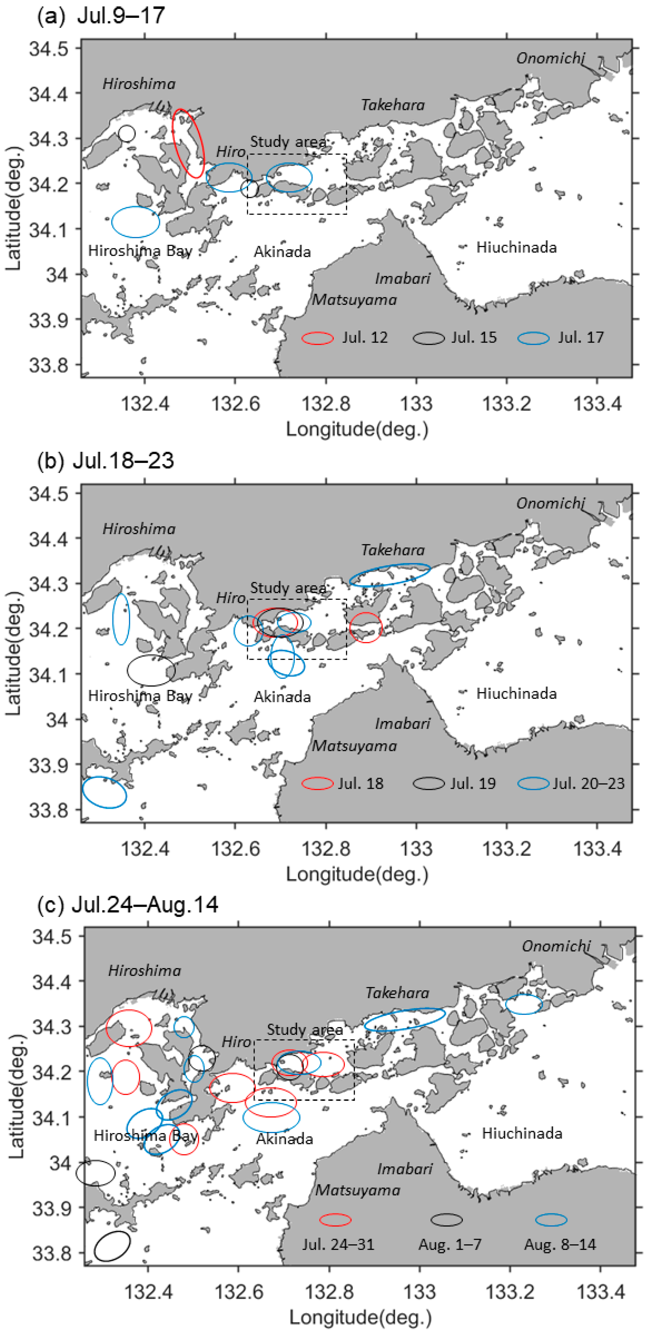
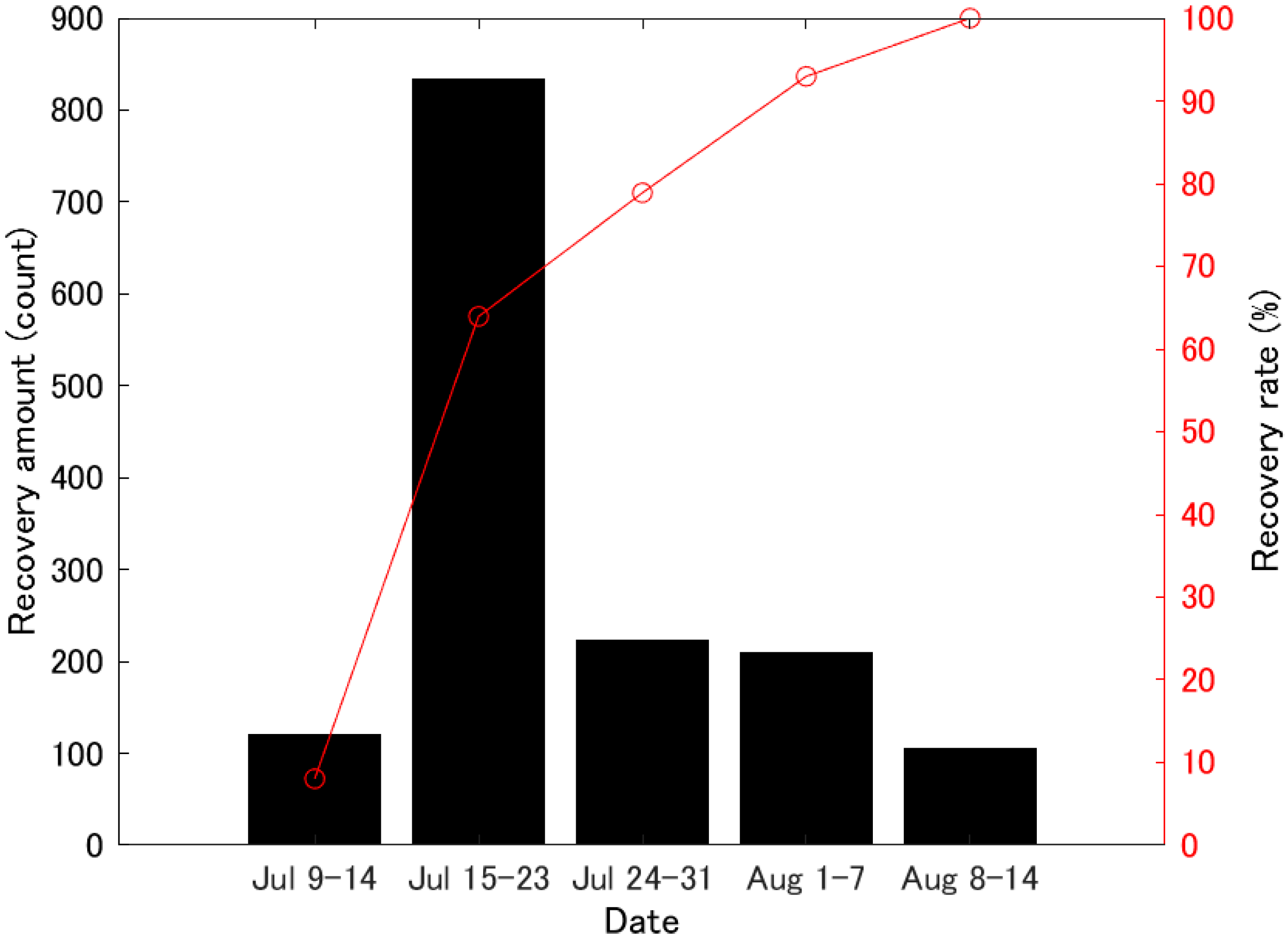
3.1. Marine Debris Collection Status by Cleaning Ships

Figure 3 shows the temporal change of marine debris distribution (over about 1 month) after the heavy rain event (see source information listed in Table 2). An overview of the marine debris acquisition locations determined by the cleaning ships is shown in the figure. Figure 3a,b shows the distribution of marine debris acquisition positions in the first half of the study period (i.e., 9 July to 23 July 2018), and Figure 3c shows the distribution of marine debris acquisition positions in the second half (i.e., 24 July to 14 August 2018). These figures show that, throughout this period, marine debris was floating in the same water area of the Seto Inland Sea off the coast of Hiroshima Prefecture. The debris frequently accumulated, in particular, in the area surrounded by the land and islands in the northern part of Aki Nada (the water area surrounded by the dotted line in Figure 3). Figure 4 summarizes the amount of garbage collected (mainly plant fragments) every week during this period. Assuming that 100% of the marine debris was collected by 14 August, the recovery rate was about 10% by 14 July, but more than 60% was recovered by 23 July. Thereafter, the amount of debris collected continued to decrease every week.

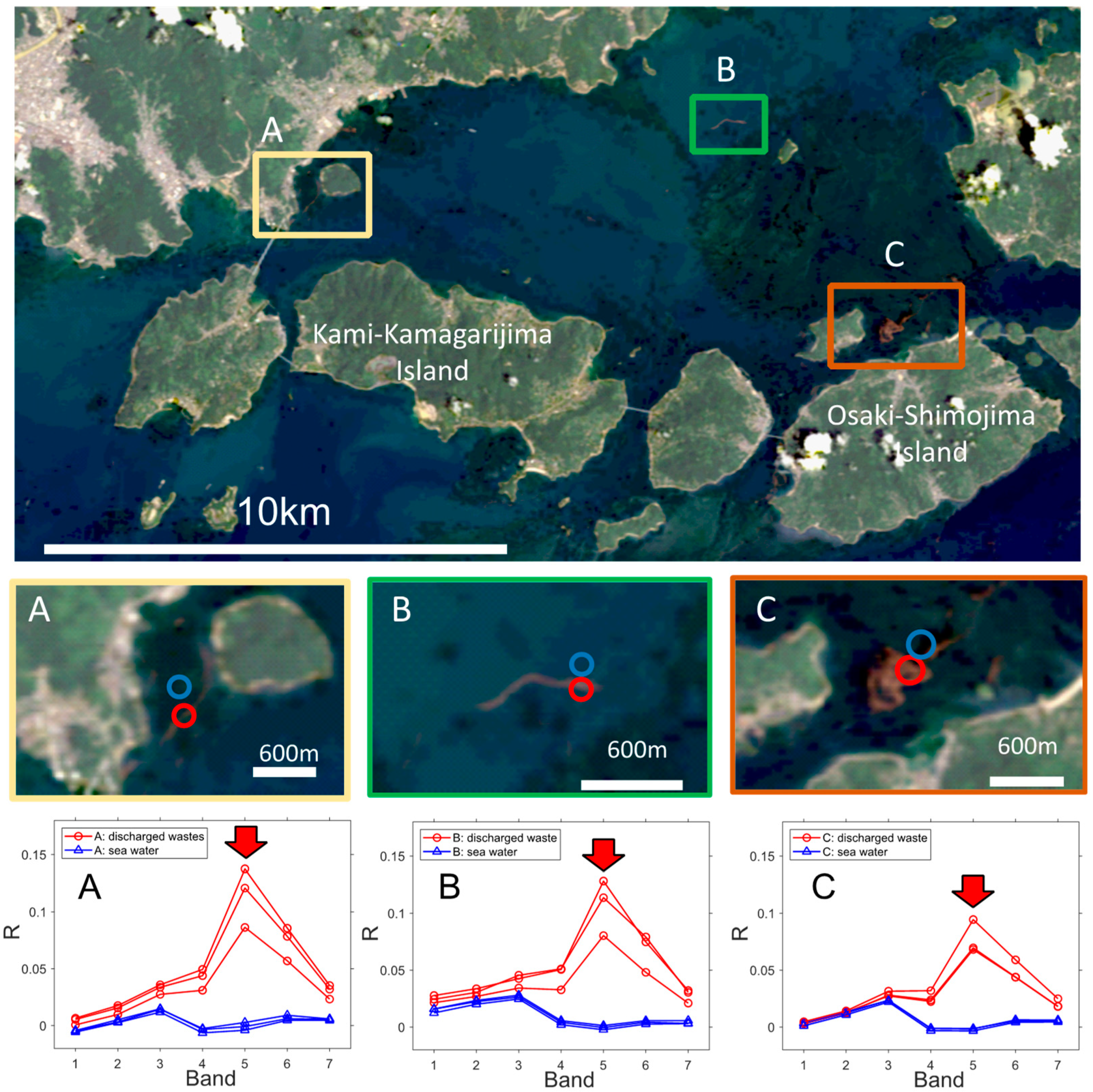
3.2. Spectral Characteristics of Marine Debris

Figure 5 shows an RGB color composite image of the Landsat-8 image taken on 9 July 2018, immediately after the heavy rain in the study area. This image shows floating objects that look red in color (examples: A, B, and C in Figure 5). The spectral reflectance characteristics extracted from the images at these three points are shown at the bottom of Figure 4. At each point, the spectral reflectance of three points of suspended matter (marked by red circles) and three points of background water (marked by blue circles) were obtained. From these spectral reflectance values, the spectral reflectance (red line) of the suspended matter was characterized by high reflectance in band 5 (central wavelength 865 nm). In addition, the reflectance gradually increased toward the long wavelength from band 1 to band 4, and the positive slopes of band 4 (central wavelength 655 nm) and band 5 were high. By contrast, the spectral reflectance of the background water was stable with a value lower than that of the suspended matter (blue lines in the bottom panels of Figure 5). With band 3 (central wavelength 560 nm) as the maximum value, the reflectance values at longer wavelengths (bands 4–7) were smaller than those at shorter wavelengths (bands 1 and 2). For bands 4–7, the reflectance values increased with wavelength. The slopes of band 4 and band 6 (central wavelength 1610 nm) used as the baseline of FAI tended to be similar for suspended matter and background clear water.
Figure 6 shows the measured spectral reflectance characteristics of marine debris along the coast of Hiroshima Prefecture. Figure 6a shows the measured original hyperspectral data, and Figure 6b shows the data obtained by extracting only the Landsat-8 band data. Unlike the results shown in Figure 6, driftwood targeted in this study had the maximum value in band 6; however, the difference between bands 4 and 5, which is the basis of the height of FAI, is considerably larger than that between other substances.

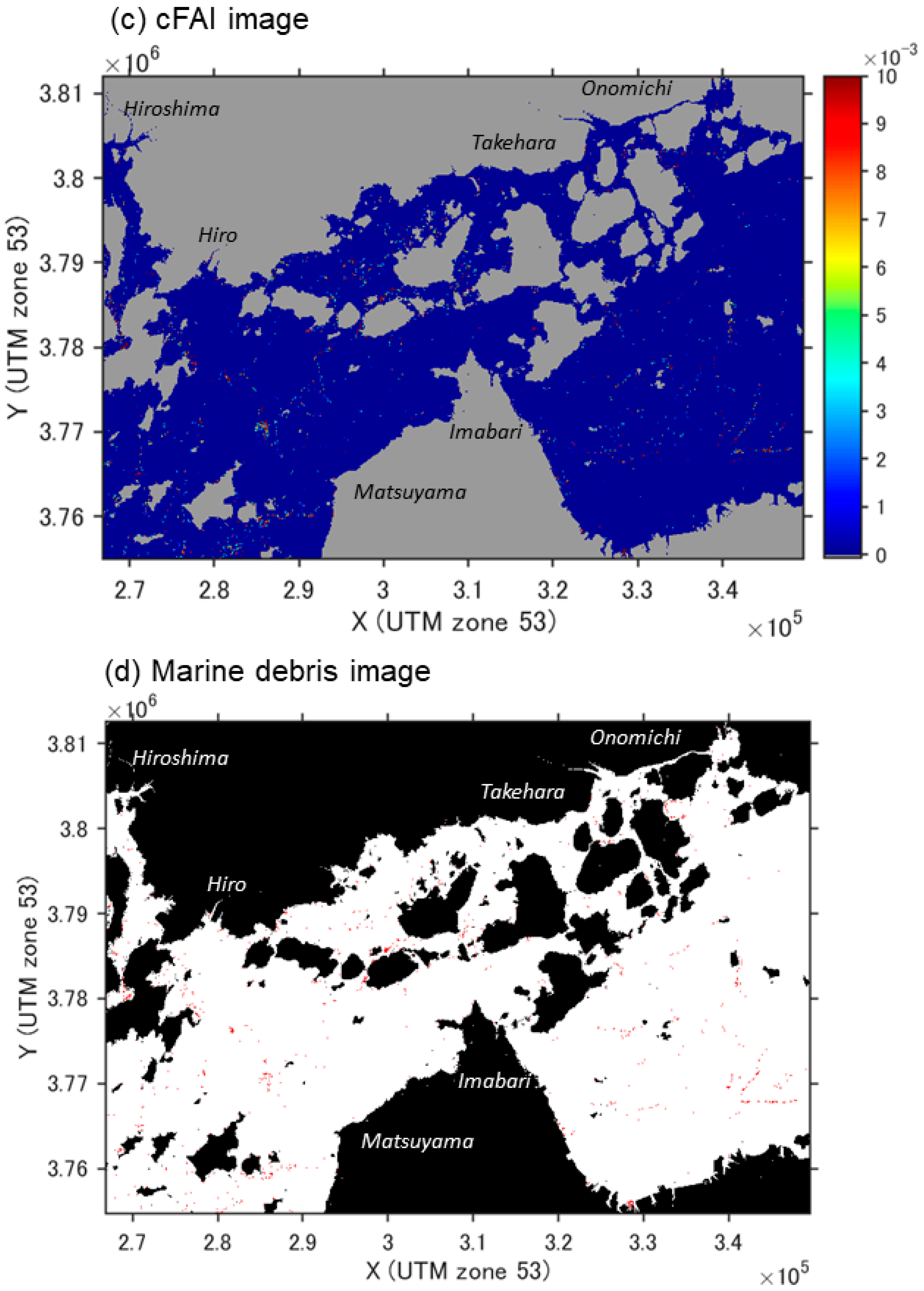
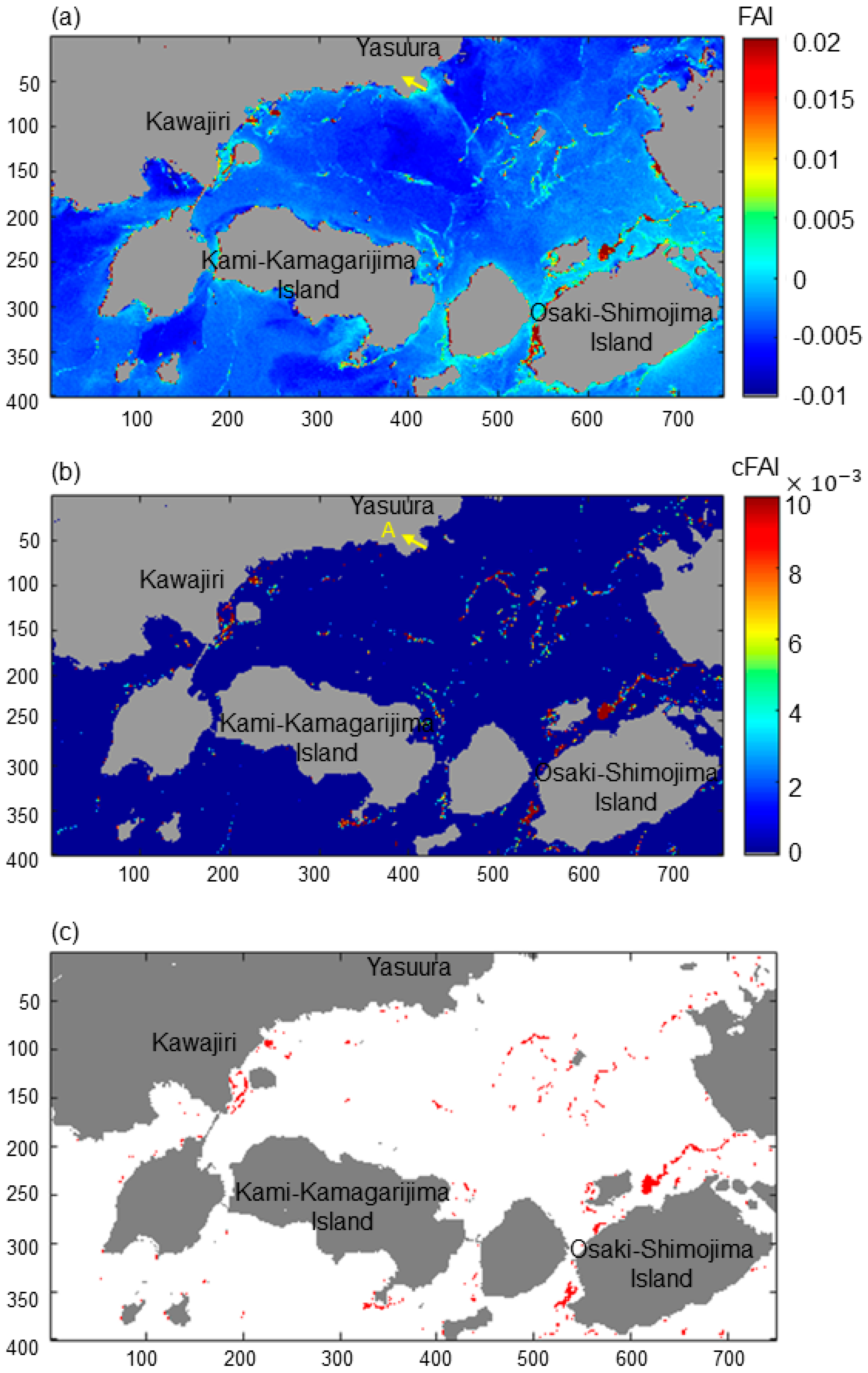
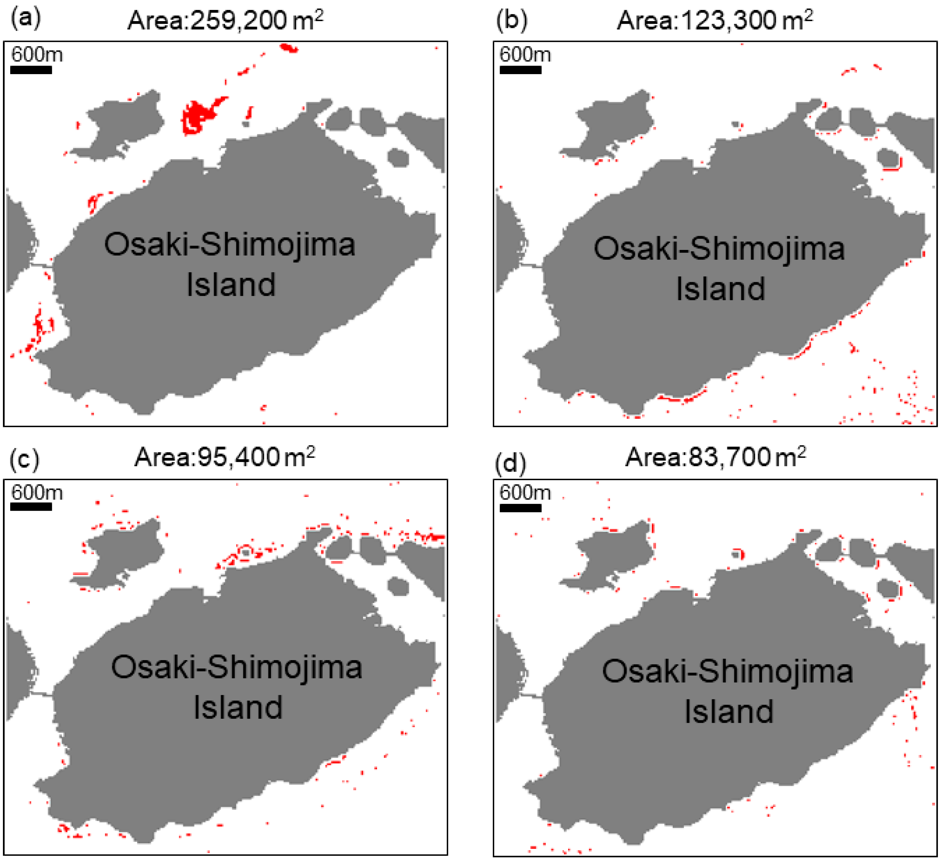
3.3. Marine Debris Detection Results Obtained Using Satellite Data

Figure 7 shows (a) FAI, (b) cFAI and (c) marine debris images calculated from Landsat-8 data on 9 July 2018. Similarly, Figure A1 (in Appendix A) shows the calculation results for the same wide area as that shown in Figure 3. From Figure 7 and Figure A1, we can confirm the presence of innumerable linear marine debris that cannot be visually read in Figure 5 from the FAI image in Figure 7a. However, it is possible to confirm a high FAI water area that is difficult to distinguish from the background water, such as water area A. In the cFAI image in Figure 7b, only marine debris, which excludes the influence of background water, was detected. In the automatic binarized image of Figure 7c, the relatively high cFAI value detected by cFAI can be clearly observed.
Figure 8 shows the threshold comparison of cFAI when the Otsu method is applied to the acquired images of locations near Osaki-Shimojima at (a) 9 July, (b) 16 July, (c) 25 July and (d) 1 August 2018. The cFAI thresholds determined by using the Otsu method show similar values with small differences for each date (0.002 to 0.008). Without the use of the Otsu method, since the distribution of the cFAI histogram is not a bimodal distribution but a continuous one, it is difficult to determine the threshold value by trial and error. Furthermore, when we applied the Otsu method for FAI and cFAI on 9 July 2018, as shown in Figure 9, a considerably larger threshold value was obtained for FAI (0.06) than for cFAI (0.008). With such high threshold for FAI (0.06), most of the suspended matter could not be detected from the corresponding FAI image (see Figure 7a).
Figure 10 shows the change in marine debris distribution near Osaki-Shimojima detected using the cFAI threshold as shown in Figure 7. Figure 10 shows that within this range, on 9 July, the distribution extended 259,200 m2 (about 0.26 km2), and marine debris continued to decrease every week. About 3 weeks later, on 1 August, the debris extended only about 83,700 m2 (0.08 km2), which is about one-fourth of the extent on 9 July. In addition, the significant marine debris accumulation seen in the northern part of Osaki-Shimojima Island (point C in Figure 5) on 9 July was not observed 1 week later on 16 July.

4. Discussion

4.1. Validity of the FAI-Based Method for Marine Debris Detection

The spectral characteristics of marine debris as obtained from Landsat-8 images are characterized by high reflectance in band 5 (around 865 nm) as shown in Figure 5. These characteristics are almost identical to the spectral characteristics of the floating marine algae detected using the FAI [9]. Therefore, it can be concluded that marine debris is detected relatively reasonably by FAI, as shown in Figure 7a. Conversely, the spectral characteristics of driftwood measured along the coast reach their maximum value in band 6 (around 1620 nm) as evident in Figure 6. This means that if driftwood floats in the sea without getting wet, it is better to consider a method for detecting marine debris using band 6. However, it is probable that most of the marine debris that flowed out after the heavy rain in the studied event was pieces of wet wood or thin pieces of wood such as reeds (see the images provided in the sources listed in Table 2). Oyama et al. [22] analyzed the measured spectral reflectance from 400 to 2400 nm and Landsat-5 data of large aquatic plants to observe the maximum reflectance near 1600 nm (Landsat-5 band 5). The FAI showed the effectiveness of separation of the target from the background water. These facts indicate that the FAI-based method is appropriate for marine debris detection. Note that, in this study, we did not intend precise classification of the types of debris. The detected debris (in Figure 7 and Figure 10) included multiple types of debris that have red edge characteristics. For the purpose of classification of marine debris, Biermann et al. [23] suggested that the use of NDVI leads to better classification results than the use of FAI (FDI; floating debris index in their paper).

4.2. Validity of Marine Debris Detection by cFAI and Otsu Methods

Figure 7a shows that the detection of marine debris by the original FAI method [9] yields many places where the values of marine debris and background water are similar. In particular, when the background of the marine debris was seawater that has become turbid because of heavy rain, it was easier to extract marine debris using cFAI, as seen from Figure 7b and Figure 9. This indicates that the methods of Hu et al. [15] are effective for marine debris extraction. When setting cGFAI that calculates the spatial gradient of reflectance, images with a relatively low resolution, such as MODIS data, may be more effective for detecting large-scale marine debris. This is because if the spatial resolution is too high, the gradient will be zero. However, most of the marine debris treated in this study was linearly distributed, and the scale was relatively small (Figure 7a); hence, it is considered that cGFAI treatment was not very difficult. Moreover, the histogram of cFAI in the target water area (Figure 8) clearly shows that it is difficult to determine the threshold value objectively from the shape. The Otsu method automatically determines the threshold value and provides reliable results such as those shown in Figure 7c and Figure 10. Thus, its use as an automatic threshold value determination in the event of such a rainfall disaster is validated.

4.3. Reason for Change in the Amount of Marine Debris Detected

On the premise that the marine debris collected was the total amount present, the rate of recovery of the marine debris by the cleaning ships by 14 July was about 10%; however, by the end of July, about 80% of the marine debris was recovered, as shown in Figure 4. Figure 10 shows that the amount of debris recovered decreased. A large amount was recovered on 9 July, while one-fourth of that amount was recovered on 1 August. This result is assumed to be the effect of marine debris collection by the cleaning ships and the result of some of the debris being washed away to the open ocean or settling on the seabed because of the strong tidal current [16,17] in the Seto Inland Sea.

4.4. Limitations of Marine Debris Detection Using Landsat-8 Data

In the event of a disaster, it is important to grasp the current situation of debris distribution over a wide area, and, as shown in this study, the Landsat-8 data are useful for this purpose. A limitation is its temporal resolution; the observation cycle of Landsat-8 is 16 days, and even if overlapping paths are present, as in the present case, the observation frequency is only about once a week. Hence, marine debris locations detected by Landsat-8 data are approximate information that cannot be completely relied upon for practical recovery works. This is because the tidal current is strong in the Seto Inland Sea, and the marine debris is quickly displaced from the locations detected by Landsat-8 data. As shown in Figure 10, the large amount of marine debris identified on 9 July is not found in the data after a week. While we presume that the cleaning ship recovered the marine debris during this period, it is possible that it was dispersed from that area by the strong tidal currents. The fate of this marine debris (in Figure 10a) was not provided by the weekly Landsat-8 data in this study. In the Seto Inland Sea, which has strong tidal currents, we believe that at least hourly images are required to follow marine debris. Providing realtime-processed debris locations on an hourly basis helps aids in efficient recovery.
There are satellites and sensors that provides hourly images. For example, the Geostationary Ocean Color Imager (GOCI) onboard the COMS satellite is a satellite sensor with a high repeat cycle and can capture images at 1-h intervals. Although GOCI does not have a band corresponding to band 6 of Landsat-8, Son et al. [24] and Qiu et al. [25] have made it possible to employ GOCI data to detect floating algae using FAI. Therefore, it can be assumed that marine debris can be detected at an early stage. However, because the spatial resolution of GOCI is 500 m, only large marine debris can be detected. Landsat-8 has a spatial resolution of 30 m, enabling it to detect marine debris better than GOCI, but it is still difficult to detect small-scale marine debris. Using sensors with insufficient spatial resolution would lead to the underestimation of amounts of marine debris. However, satellites or sensors with both sufficient temporal and spatial resolution are not yet available. Therefore, research that combines Sentinel-2 mission with a spatial resolution of 10 m and satellites with a spatial resolution of about 50 cm to 3 m such as DOVE, WorldView, and Pleiades [26] will be important.

5. Conclusions

In this study, an attempt was made to reproduce the actual state of marine debris distribution in the Seto Inland Sea off the coast of Hiroshima Prefecture during the heavy rains in July 2018. For this purpose, marine debris acquisition information from cleaning ships and Landsat-8 images was used. The following conclusions were drawn from our work.
  • From the data acquired by the cleaning ships on multiple days, the distribution of marine debris immediately after the heavy rain was approximated. In particular, the debris was concentrated in the water area surrounded by land and islands in the northern part of Aki Nada.
  • From the spectral reflectance data of Landsat-8 level-2, we confirmed that the marine debris had a high peak reflectance in band 5 (central wavelength 865 nm).
  • Unlike the original FAI method, the cFAI method enabled us to remove the background water signals from the Landsat-8 images.
  • The Otsu method for the automatic binarization of cFAI was effective in detecting marine debris from Landsat-8 images because it set an appropriate threshold value.
In the future, we would like to use data such as GOCI data, which obtains data more frequently than Landsat, and WorldView-2, which has a high spatial resolution. Using such data, we will aim to track the detailed movement of marine debris (movement vector) and achieve higher spatial resolution. In recent years, heavy rainfall disasters have occurred frequently in Japan, and we would like to validate the effectiveness of this method in water areas other than the Seto Inland Sea.

Author Contributions

Conceptualization and methodology, Y.S.; formal analysis and visualization, S.S.; supervision, Y.S., N.T. and H.I.; investigation and writing—original draft preparation, S.S., Y.S. and N.T.; writing—review and editing, all authors. All authors have read and agreed to the published version of the manuscript.

Funding

This research was funded by JSPS KAKENHI Grant Numbers 19H04292, 20KK0141, and 21H03650.

Acknowledgments

The Landsat-8 product used in this paper was supplied by the Earth Explorer system (https://earthexplorer.usgs.gov/, accessed on 1 November 2021) of USGS.

Conflicts of Interest

The authors declare no conflict of interest.

Appendix A

Figure A1. (a) True color, (b) FAI, (c) cFAI, and (d) marine debris images calculated from Landsat-8 data acquired on 9 July 2018. Results over a wider area than that in Figure 7 are shown.
Remotesensing 13 05048 g0a1aRemotesensing 13 05048 g0a1b

References

  1. Tsuguti, H.; Seino, N.; Kawase, H.; Imada, Y.; Nakaegawa, T.; Takayabu, I. Meteorological overview and mesoscale characteristics of the Heavy Rain Event of July 2018 in Japan. Landslides 2019, 16, 363–371. [Google Scholar] [CrossRef]
  2. Hirota, K.; Konagai, K.; Sassa, K.; Dang, K.; Yoshinaga, Y.; Wakita, E.K. Landslides triggered by the West Japan Heavy Rain of July 2018, and geological and geomorphological features of soaked mountain slopes. Landslides 2019, 16, 189–194. [Google Scholar] [CrossRef]
  3. Opfer, S.; Arthur, C.; Lippiatt, S. NOAA Marine Debris Shoreline Survey Field Guide; NOAA Marine Debris Program: Silver Spring, MD, USA, 2012. [Google Scholar]
  4. Moy, K.; Neilson, B.; Chung, A.; Meadows, A.; Castrence, M.; Ambagis, S.; Davidson, K. Mapping coastal marine debris using aerial imagery and spatial analysis. Mar. Pollut. Bull. 2012, 132, 52–59. [Google Scholar] [CrossRef]
  5. Kubota, M. A mechanism for the accumulation of floating marine debris north of Hawaii. J. Phys. Oceanogr. 2019, 24, 1059–1064. [Google Scholar] [CrossRef]
  6. Isobe, A.; Iwasaki, S.; Uchida, K.; Tokai, T. Abundance of non-conservative microplastics in the upper ocean from 1957 to 2066. Nat. Commun. 2019, 10, 417. [Google Scholar] [CrossRef] [PubMed] [Green Version]
  7. Komatsu, T.; Sagawa, T.; Sawayama, S.; Tanoue, H.; Mohri, A.; Sakanishi, Y. Mapping is a key for sustainable development of coastal waters: Examples of seagrass beds and aquaculture facilities in Japan with use of ALOS images. In Sustainable Development: Education, Business and Management—Architecture and Building Construction—Agriculture and Food Security; Books on Demand: Norderstedt, Germany, 2012; pp. 145–160. [Google Scholar]
  8. Murata, H.; Komatsub, T.; Yonezawac, C. Detection and discrimination of aquacultural facilities in Matsushima Bay, Japan, for integrated coastal zone management and marine spatial planning using full polarimetric L-band airborne synthetic aperture radar 5. Int. J. Remote Sens. 2019, 40, 5141–5157. [Google Scholar] [CrossRef]
  9. Hu, C. A novel ocean color index to detect floating algae in the global oceans. Remote Sens. Environ. 2009, 113, 2118–2129. [Google Scholar] [CrossRef]
  10. Hu, C.; Li, D.; Chen, C.; Ge, J.; Muller-Karger, F.E.; Liu, J.; Yu, F.; He, M.X. On the recurrent Ulva prolifera blooms in the Yellow Sea and East China Sea. J. Geophys. Res. 2010, 115, C05017. [Google Scholar] [CrossRef] [Green Version]
  11. Cózar, A.; Aliani, S.; Basurko, O.C.; Arias, M.; Isobe, A.; Topouzelis, K.; Rubio, A.; Morales-Caselles, C. Marine litter windrows: A strategic target to understand and manage the ocean plastic pollution. Front. Mar. Sci. 2021, 8, 571796. [Google Scholar] [CrossRef]
  12. Sato, H.; Takeda, K.; Matsumoto, K.; Anai, H.; Yamakage, Y. Efforts for disaster prevention/mitigation to protect society from major natural disasters. Fujitsu Sci. Tech. J. 2016, 52, 107–113. [Google Scholar]
  13. Cheng, J.W.; Mitomo, H. Multi-channel information dissemination for disaster evacuees–the case of the 2016 Kumamoto Earthquake in Japan. In Proceedings of the 29th ITS European Conference, Trento, Italy, 1–4 August 2018. [Google Scholar]
  14. Garcia, R.A.; Fearns, P.; Keesing, J.K.; Liu, D. Quantification of floating macroalgae blooms using the scaled algae index. J. Geophys. Res. 2013, 118, 26–42. [Google Scholar] [CrossRef] [Green Version]
  15. Hu, L.; Zeng, K.; Hu, C.; He, M.X. On the remote estimation of Ulva prolifera areal coverage and biomass. Remote Sens. Environ. 2019, 223, 194–207. [Google Scholar] [CrossRef]
  16. Takasugi, Y.; Hoshika, A.; Noguchi, H.; Tanimoto, T. The role of tidal vortices in material transport around straits. J. Oceanogr. 1994, 50, 65–80. [Google Scholar] [CrossRef]
  17. Takeoka, H. Progress in Seto Inland Sea research. J. Oceanogr. 2002, 58, 93–107. [Google Scholar] [CrossRef]
  18. Hashimoto, R.; Tsuchida, T.; Moriwaki, T.; Kano, S. Hiroshima Prefecture geo-disasters due to Western Japan Torrential rainfall in July 2018. Soils Found. 2020, 60, 283–299. [Google Scholar] [CrossRef]
  19. Garaba, S.P.; Dierssen, H.M. Hyperspectral ultraviolet to shortwave infrared characteristics of marine-harvested, washed-ashore and virgin plastics. Earth Syst. Sci. Data 2020, 12, 77–86. [Google Scholar] [CrossRef] [Green Version]
  20. Moshtaghi, M.; Knaeps, E.; Sterckx, S.; Garaba, S.; Meire, D. Spectral reflectance of marine macroplastics in the VNIR and SWIR measured in a controlled environment. Sci. Rep. 2021, 11, 5436. [Google Scholar] [CrossRef]
  21. Otsu, N. A threshold selection method from gray-level histograms. IEEE Trans. Syst. Man. Cybern. 1979, 9, 62–66. [Google Scholar] [CrossRef] [Green Version]
  22. Oyama, Y.; Matsushita, B.; Fukushima, T. Distinguishing surface cyanobacterial blooms and aquatic macrophytes using Landsat/TM and ETM+ shortwave infrared bands. Remote Sens. Environ. 2015, 157, 35–47. [Google Scholar] [CrossRef]
  23. Biermann, L.; Clewley, D.; Martinez-Vicente, V.; Topouzelis, K. Finding plastic patches in coastal waters using optical satellite data. Sci. Rep. 2020, 10, 5364. [Google Scholar] [CrossRef] [PubMed] [Green Version]
  24. Son, Y.B.; Choi, B.J.; Kim, Y.H.; Park, Y.G. Tracing floating green algae blooms in the Yellow Sea and the East China Sea using GOCI satellite data and Lagrangian transport simulations. Remote Sens. Environ. 2015, 156, 21–33. [Google Scholar] [CrossRef]
  25. Qiu, Z.; Li, Z.; Bilal, M.; Wang, S.; Sun, D.; Chen, Y. Automatic method to monitor floating macroalgae blooms based on multilayer perceptron: Case study of Yellow Sea using GOCI images. Opt. Express 2018, 26, 26810–26829. [Google Scholar] [CrossRef] [PubMed]
  26. Qi, L.; Hu, C.; Mikelsons, K.; Wang, M.; Lance, V.; Sun, S.; Barnes, B.B.; Zhao, J.; Van der Zande, D. In search of floating algae and other organisms in global oceans and lakes. Remote Sens. Environ. 2020, 239, 111659. [Google Scholar] [CrossRef]
Figure 1. Location map of the study area with the orbital information of Landsat-8. Points labeled ①, ②, ③, and ④ indicate the positions of Ohta River, Ashida River, Kurose River, and Nuta River, respectively.
Remotesensing 13 05048 g001
Figure 2. (a) Flow of marine debris extraction by Landsat-8 data and (b) conceptual diagram of corrected floating algae index (cFAI) threshold determination by the Otsu method.
Remotesensing 13 05048 g002
Figure 3. Summary of marine debris acquisition locations as determined by the cleaning ships.
Remotesensing 13 05048 g003
Figure 4. Time series of the amount of marine debris collected by the cleaning ships. The bar graph and line graph show the number of plant fragments and the recovery rate, respectively.
Remotesensing 13 05048 g004
Figure 5. Landsat-8 RGB color composite image acquired on 9 July 2018 immediately after the heavy rainfall disaster. The areas labeled A, B, and C in the (top panel) are enlarged in the (middle panels). The (bottom panels) show the spectral characteristics of the pixels in the red circle (suspended matter) and blue circle (background water) in each middle panel.
Remotesensing 13 05048 g005
Figure 6. Example of spectral characteristics of the marine debris collected from the coast. (a) Hyperspectral data and (b) the data of Ladsat-8 band only.
Remotesensing 13 05048 g006
Figure 7. (a) FAI, (b) cFAI, and (c) marine debris images calculated from Landsat-8 data acquired on 9 July 2018.
Remotesensing 13 05048 g007
Figure 8. Comparison of the cFAI thresholds obtained by the Otsu method for four periods: (a) 9 July (b) 16 July (c) 25 July, and (d) 1 August 2018.
Remotesensing 13 05048 g008
Figure 9. Comparison of the thresholds of FAI and cFAI data obtained by the Otsu method for 9 July 2018.
Remotesensing 13 05048 g009
Figure 10. Changes in the marine debris distribution near Osaki-Shimojima Island using Landsat-8 data. The debris distributions on (a) 9 July, (b) 16 July, (c) 25 July, and (d) 1 August 2018 are shown.
Remotesensing 13 05048 g010
Table 1. Bands of landsat-8 operational land imager (OLI) level 2.
BandWavelength (μm)Spatial Resolution (m)
10.43–0.4530
20.45–0.5130
30.53–0.5930
40.64–0.6730
50.85–0.8830
61.57–1.6530
72.11–2.2930
Table 2. List of published reports (press releases; accessed on 1 November 2021) on marine debris collections by cleaning ships from the Ministry of Land, Infrastructure, Transport and Tourism after the heavy rain in July 2018.
Publisher’s Note: MDPI stays neutral with regard to jurisdictional claims in published maps and institutional affiliations.

