1. Introduction
Air temperature (Ta), defined as the temperature at 2 m above the land surface, is one of the most important variables in regional and global weather models of the terrain and its characteristics [
1,
2]. Ta affects the rates of biotic processes in the ecosystem, including phonologies, growth, carbon, fixation, insolation, and respiration through vegetation–moisture/water relationships [
3,
4,
5,
6,
7,
8]. Thus, Ta is used in many areas of research that monitor climate change, global warming, and abnormal temperature phenomenon. The accuracy of Ta readings is essential, but it only represents a relatively small area because it is measured locally at in-situ stations.
In general remote sensing, most of retrieved data from satellite data were retrieved using various ways in a large area like atmosphere, land and ocean. For example, threshold method was generally used in various satellites cloud mask algorithm, which needed to retrieve existence of cloud in each pixel [
9,
10]. And satellite data were used to retrieve the state of various environments, such as Land Surface Temperature (LST), using the characteristics of wavelengths. And satellite also can be used as input data in climate model to retrieve information over the Ocean are crucial to improve the numerical weather prediction model’s initial condition to predict severe weather events like tropical cyclones and hurricanes accurately in ocean area [
11,
12]. LST which means the radiological surface temperature, depends on the surface conditions, such as landcover, land moisture, and air conditions, and is one of the most important variables of ecosystems [
13]. In remote sensing, LST is retrieved from satellite and sensor data, and can represent a large area because it is retrieved by satellite observation. And Surface observation of satellite can be used to extracting information of near-surface environmental conditions such as Ta because satellite observation can represent better spatial coverage [
14,
15,
16,
17]. Therefore, many studies proposed Ta retrieval method with LST of satellite data to retrieve Ta in a large area [
17,
18,
19,
20]. In many studies and satellite algorithms, LST is calculated by observing the energy emitted from Earth’s surface through satellite remote sensing. To retrieve LST, these studies and algorithms commonly use the split-window algorithm. The split-window algorithm, generally known as the LST retrieval algorithm, is based on water vapor absorption obtained using two infrared (IR) channels, specifically, the atmospheric window channels corresponding to 11 and 12 µm.
Ta is generally only representative of the small area surrounding the measurement location, as opposed to that covered by satellite imagery. Because Ta and LST are highly correlated, it may be possible to retrieve Ta from the readings of the two IR channels (11 and 12 µm) used for LST retrieval method. In [
17,
18,
19,
20], Ta has been measured from LST by multiple regression. But there is no official LST data from Landsat-8 therefore we needed to use other data which was validated. Moreover, studies in similar study area can be found in [
17,
20], but as I mentioned these studies used the multiple regression method. Therefore, we investigated the ability to retrieve Ta with IR channels data using a deep neural network (DNN) to try to find another method.
A DNN is an artificial neural network (ANN) consisting of several hidden layers between an input layer and an output layer. DNNs, like ordinary ANNs, can model complex nonlinear relationships. For example, in a DNN structure for object identification, each object can be represented as a hierarchical organization of the basic elements of the image. At this point, additional layers can incorporate the characteristics of the lower layers, which are gradually aggregated. These features of DNNs allow complex data to be modeled with fewer units (units, nodes) compared to the modeling via ANNs [
21].
To estimate Ta with IR channels, several variables must be chosen for applying the DNN. Here, we focused on variables related to LST, specifically, the Normalized Difference Vegetation Index (NDVI) and the Normalized Difference Water Index (NDWI). We tested each variable in the DNN to identify the best variable for retrieving Ta with high accuracy.
2. Study Area
The study area included South Korea, extending from about 33° N to 39° N and from 124° E to 130° E (
Figure 1). South Korea is part of Northeast Asia, which experiences four seasons with considerably different characteristics regarding atmospheric readings. There are four air masses that affect the seasons of South Korea: the North Pacific air mass, characterized by a very high temperature and very high humidity in summer; the Siberian air mass, characterized by a very low temperature and low humidity in winter; the Yangtze-river air mass, which comes from China and brings warm temperatures in spring and autumn; and the Okhotsk Sea air mass, characterized by cool temperatures and high humidity. The Okhotsk Sea air mass brings rain to South Korea during the rainy season in summer and early autumn. Additionally, South Korea is surrounded on three sides by the sea; thus, both land and sea conditions affect the region’s temperature. And especially, previous studies referred effect to cold surges by arctic oscillation [
22,
23]. We thought if we can retrieve Ta from satellite, the result can be used to analyze effects of arctic oscillation. For this reason, we chose South Korea as our study area to investigate the correlation between Ta and various conditions in the area.
3. Data
3.1. Ta Data
In South Korea, the Korea Meteorological Administration operates an in-situ data collecting system, the Automated Synoptic Observing System (ASOS). ASOS has 102 locations throughout South Korea which have various land types, thus, we divided the land type into four categories, urban, plain, forest, mixed. Urban means case that ASOS point was surrounded by urban structures, such as building, factory, road. Plain means case that ASOS point was surrounded by crop land. Forest means case that ASOS point was surrounded by trees including mountains. Mixed means case that two or more of the three are mixed (
Figure 1). And ASOS collects meteorological data, including temperature, air pressure, wind, humidity, evapotranspiration, and snow data, from every ASOS point at certain times throughout the day. ASOS Ta, Ta quality, latitude, and longitude were collected on an hourly basis from 2014 to 2017. We used ASOS Ta data as input and validation data and this allowed the data to be matched with other datasets, including that of Landsat-8. And we also used ASOS data from 2018 to 2019 for testing applicability of model which was made in this study.
3.2. Landsat-8 Data
Landsat satellites have been conducting remote sensing missions since 1972. Landsat-8 observes the earth in near-polar orbit and its temporal resolution is longer the satellite in geostationary orbit. The temporal resolution of Landsat-8 is 16 days, this means retrieves data over the entire Earth in 16 days using two sensors: the Operational Land Imager (OLI) and the Thermal Infrared Sensor (TIRS) and the period that satellite observes the same area is 16 days. The OLI has 30-m resolution for surface reflectance and the TIRS has 100 m spatial resolution for brightness temperature (
Table 1). The United States Geological Survey processes TIR data with 30 m spatial resolution through resampling [
24]. To calculate the variables of Landsat-8 data, we used L2 data and top-of-canopy reflectance data, referring to the surface reflectance data-applied atmospheric correction of OLI data used to remove atmospheric effects, which is important for land surface observations [
25,
26]. In addition, we used L1 top-of-atmosphere data from the TIRS. The brightness temperature of TIRS and the reflectance of OLI were used by calculating binary data arriving from satellites. Therefore, we thought that verification of the accuracy of the data was secured. We collected 334 scenes each of L1 and L2 data for matching up with ASOS Ta data; notably, the observation time offset was less than 30 min. All Landsat-8 data included reflectance or brightness temperature information and QA (Quality Assurance) information. The QA information was made with 16 bits, and you can check the condition of the pixel by interpreting each bit. Therefore we were checked to ensure good and clear conditions. [
27]
4. Methods
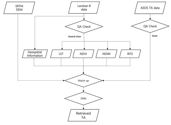
This work aimed to apply satellite data and in-situ data to the DNN model to produce an optimal DNN model for Ta retrieval (
Figure 2). First, we conducted a quality check of the collected Landsat-8 data. And then, we used Landsat-8 data for application to the DNN model. All data of this study have clear weather condition and good observation condition. For this reason, we needed to check the condition of all data. Therefore we checked quality before we retrieved NDVI and NDWI in good quality and we set Band10, Band11, NDVI and NDWI to the DNN model.
ASOS Ta was served both temperature, QA, spatial information such as latitude and longitude. Therefore, we check quality with QA data and we set Ta data to the DNN model.
Satellite-based Landsat-8 is available in “Scene” form; however, ASOS Ta assumes the “Point” form, as it is ground truth data. For this reason, we performed spatial match- up based on the ASOS Ta data to produce optimized data for input into the DNN model. The characteristics of satellite observations are such that temporal and spatial matching is essential. Therefore, the nearest ASOS Ta data were obtained based Landsat-8 observed the research area and data of the difference in observation time within 30 min. Because Landsat-8 observes South Korea at 11:00 (KST) every 16 days, we collected ASOS Ta data from 2014 to 2017 to obtain as much data as possible. Spatial matching of the Landsat-8 and ASOS Ta data required calculating the Great Circle Distance (GCD) method with latitudes and longitudes of Landsat-8 and ASOS points. As a result, all inputs had complete spatiotemporal matching of the dependent variables of ASOS Ta and the input variables of Band 10, Band 11, NDVI, and NDWI, with a total of 3139 produced data.
A DNN performs verifications of the application results by randomly dividing all input variables by 70% and 30% ratios. Using 70% of the data, the application of the DNN model first tested the conditions that could affect the model outcome, including various input variables, nodes, batch sizes, and epochs, and determined the optimal conditions with the remaining 30% of the data, in an attempt to yield the most accurate Ta retrieval. In validation, we validated throughout spatial matching the retrieved Ta and ASOS Ta data with each latitude and longitude. After validation of each condition of models, we finally selected the most accurate DNN model in this study. And we additionally validated the result with various step. The first step was validated in condition of each used variable and the second step was seasonal validation, the third step was point validation which means we validated the result in various ASOS point, not combined results of all points.
Deep Neural Network
DNN is a type of machine learning in which computers form large ANNs that resemble the human brain. Deep learning provides learning algorithms and an ever-increasing amount of data to large ANNs, thus allowing for continuous improvement in their ability to “think” and “learn” data. And ANN is used various studies using satellite data in remote sensing, for example, it was used to retrieve the surface rain rate [
28,
29,
30,
31].
The word “deep” in DNN refers to the multiple layers of neural networks that accumulate over time. Deep neural networks result in better performance. Deep learning is an artificial intelligence technology that combines more active unsupervised learning with conventional supervised learning that requires human intervention, allowing computers to learn on their own like humans. Technically, deep learning is a collection of machine learning that teaches computers how to think like people.
DNNs are the new norm in signal and data processing, achieving state-of-the-art performance in image, audio, and natural language understanding; additionally, they are used to enhance remote sensing techniques [
32]. Deep learning performs well in various kinds of pattern recognition, based on classification and retrieval [
33]. Here, DNN learning should help to resolve the correlation between Ta and data obtained from Landsat-8.
5. Results
5.1. Model Condition Selection
Various factors can affect the DNN model. In this study, the optimal model was selected by comparing the differences in accuracy according to input variables, nodes, batch size, and epoch. Verification for optimal model selection was performed by randomly dividing the entire dataset into 70% and 30% portions for use as data for Ta production and verification, respectively.
5.1.1. Variables
In our DNN model, ASOS Ta was the dependent variable, and Band 10, Band 11, NDVI, and NDWI were applied as the independent variables. Changes in the independent variables affect the accuracy of the results obtained using the model. Therefore, we tested various cases of individual variables to establish the relevance of each variable.
Figure 3 shows result of correlation between Ta and each variable. To test each variable, we made 4 DNN model and Ta was applied as a dependent variable and each of Band 10, Band 11, NDVI and NDWI was applied to the model as an independent variable. We set DNN condition with 32 batch size, epoch 100, node 50 to test in same condition. And we used Colaboratory of Google, its specifications are T4 GPU, 25.51 GB RAM. We tested availability of each variable; Band 10 and Band 11 and NDVI and NDWI.
Generally, the atmospheric window is assumed to range from 8 to 12 µm; in this wavelength range, there is little absorption by the atmosphere such that it easily reaches the Earth’s surface unless absorbed by cloud. LST, as mentioned earlier, is calculated by detecting the energy of 11 and 12 µm released from the Earth’s surface to satellites, i.e., the split window method [
13,
34,
35,
36]. Emissivity must be considered, given that an uncertainty of 1% in emissivity results in an error of 0.5 K in the calculation of the LST [
37]. Ref. [
38] proposed the method to derive a log-linear relation between NDVI and we calculated emissivity using the log-linear relationship between the NDVI and ε11 from previous studies [
39,
40,
41,
42]. Emissivity of 11 µm, ε11, as given below:
The Band 10 and Band 11 represented the emissivity of the blackbody, which differs from the actual emissivity from the Earth. For this reason, Bands 10 and 11 were used by multiplying emissivity in this study. And we applied Band 10 and Band 11 with Ta to the DNN model. The result of Band 10 was shown in
Figure 3a and the R value was 0.96, and the root mean square error (RMSE) was 2.73 K and bias was 0.4819 K. The result of Band 11 was shown in
Figure 3b. The R value was 0.97, and the RMSE was 2.33 K and bias was −0.0791 K. These results were shown that Band 10 and Band 11 were highly correlated with Ta.
NDVI uses the difference in red (band4, 0.64~0.67 µm) and NIR (band5, 0.85~0.88 µm) reflectance readings to distinguish dense and sparse vegetation coverage. Dense (sparse) vegetation coverage shows high (low) NIR reflectance, which affects the NDVI (Equation (2)) Thus, the NDVI is used to resolve land surface changes as they relate to global change, the carbon cycle, land coverage/use, and terrestrial ecology research [
43]. The NDVI was obtained from data collected by the OLI from two bands (Band 2 and Band 4); each pixel has a 30-m spatial resolution. The relationship between NDVI and LST has been investigated in numerous studies [
44]. A previous study [
45] investigated LST retrieval algorithms with various NDVI-based land surface emissivity models. From these earlier studies, NDVI and LST are correlated; thus, NDVI should be related to Ta. In this study, the NDVI was calculated for each pixel and the pixel condition was checked with QA data before being included in the calculations:
And we applied NDVI with Ta to the DNN model.
Figure 3c showed result of Ta and NDVI. The R value was 0.97 and the RMSE was 2.44 K and bias was 0.7418 K. This result means NDVI was highly correlated with Ta.
LST was generally observed to be higher than Ta during the day, as the heat at the Earth’s surface was lower than that in the atmosphere [
46]. Ta values higher than LST suggest that the satellite observations may have been affected by moisture from cirrus cloud coverage or haze in the air in summer [
17,
20,
47]. In remote sensing, the NDWI represents the surface water condition and is widely used in various methods, such as those described by [
48] using NIR and short-wave IR and [
49] using green and NIR wavelengths. Our approach to inferring the surface moisture of a pixel is based on Gao’s method, as it is commonly used in remote exploration [
50,
51]. Here, we calculated the NDWI with Band 3 and Band 6 using Gao’s method (Equation (3)). NDWI was calculated for each pixel, and the pixel condition was cross-checked against QA data to ensure that the reading coincided with the appropriate NDWI reading:
And we applied NDWI with Ta to the DNN model. And result of Ta and NDWI was shown in
Figure 3d. The correlation coefficient (R) value was 0.97 and the RMSE was 2.29 K and bias was −0.0427 K. Band 10, Band 11, NDVI and NDWI were highly correlated with Ta in these tests. In all result of them, the R values were over 0.96 and the RMSEs were under 2.73 K. We confirmed availability of these variables, and selected variables as input variables of DNN model in this study.
5.1.2. Batch Size
Batch size, which exploits unit data size in applying the model once, has a significant impact on the accuracy of the DNN model. A batch size that is too small will result in a model that overfits the data, showing a high RMSE (
Figure 4). We tested the DNN model with batch sizes applied as a multiple of 2. The input variables from the LST, NDVI, and NDWI data were identified in the previous step. We confirmed an optimal batch size of 256 over the range of batch sizes tested from 32 to 1024, with epoch 10 conditions. Given a batch size of 256, the R value was over 0.94 and the lowest RMSE was 2.35 K.
5.1.3. Selected Model
In the previous steps, we selected the best conditions for the DNN model, four independent variables (Band 10, Band 11, NDVI, and NDWI), and a batch size of 256 for the highest accuracy. Using these conditions, we constructed a DNN model with 70% of the total matchup data, which were selected randomly, and validated the model with the remaining 30% (
Figure 5). We achieved an R value of 0.98 and an RMSE of 2.19 K; the mean absolute error (MAE) was 1.75 K for the DNN model, such that it exceeded the accuracy of the other conditions combined. Compared with the results of previous studies, our results showed better accuracy (
Table 2). An MAE value of 2.21 K was found by [
19] compared with 1.75 in this study. [
17] estimated Ta with 3.30 K of RMSE, lower in accuracy than this study. In [
18], the RMSE and MAE were calculated for day and night conditions; our results showed higher accuracy than those of [
19] in both RMSE and MAE. [
20] estimated Ta with water conditions using multiple regression, showing an RMSE of 2.89 K, the highest accuracy of the earlier studies; however, the RMSE was higher by about 0.7 K compared with our results.
5.2. Spatial Representativeness
Because Ta is readily altered by convection currents, the LST has a higher standard error if the Ta and LST have the same values. Conversely, surface heat transfer cannot be determined easily because there is no transmitter [
52]. In a previous study, the deviation in Ta was about 0.6 K when the horizontal distance was 6 km [
53]. Here, we tested 25 additional cases, varying in window size from 1 × 1 to 297 × 297, which corresponded to areas of 30 m × 30 m and 9 km × 9 km, respectively (
Figure 6). We checked the changes in RMSE and bias for spatial representativeness. As the window size increased, the RMSE decreased up to a 231 × 231 window size (1.95 K). There was little difference in the RMSE after reaching a window size of 132 × 132. The difference between the RMSE values of the 231 × 231 and 132 × 132 window sizes was 0.0102 K. This variability was similar for the bias. As the window size increases, the bias decreases. The lowest bias was shown for the 132 × 132 window size. As a result, we considered that the spatial representativeness was optimal for the 132 × 132 window size, representing 4 km × 4 km, with an RMSE of 1.96 K and a bias of −0.00856 K.
5.3. Analysis of Individual Variables
It was necessary to identify changes in the estimated temperature of the calculation as the variables changed. We tested the Ta difference between the retrieved Ta and the reference Ta from ASOS data for each variable (
Figure 7). When comparing the Ta difference, changes were identified for Band 10, Band 11, NDVI, and NDWI.
In
Figure 7, the Ta difference showed little change as the individual variables were varied. The slope of Band 10 was −0.015, and the slope of Band 11 was −0.0031. Thus, the changes in Bands 10 and 11 did not affect the accuracy of the temperature calculation (
Figure 7a,b). A similar pattern occurred for the NDVI and NDWI with respect to Band 10 and Band 11 (
Figure 7c,d). Their slopes were 0.4948 and 0.2225. The slopes of NDVI and NDWI were larger than those of the IR bands; however, from the small amount of changes in the NDVI and NDWI, it was determined that the change in temperature was also very small.
Because Ta exists in the form of fluids, it is necessary to verify the accuracy of seasonal Ta due to the relatively smooth delivery of temperatures to the surrounding area compared to surface temperatures. In this study, additional verification was performed for each season with RMSE and bias. Each season was divided into March, April, and May (MAM) for the spring period; June, July, and August (JJA) for the summer period; September, October, and November (SON) for the autumn period; and December, January, and February (DJF) for the winter period. There were 268, 146, 285, and 225 verified data for MAM, JJA, SON, and DJF, respectively. There was a relatively small amount of data in summer due to the presence of clouds during the rainy season and typhoon season in Korea.
The results of the verification differed seasonally as follows: MAM (2.82 K), JJA (2.27 K), SON (1.99 K), and DJF (2.00 K), based on the RMSE; and MAM (1.7859), JJA (0.0085), SON (0.0699), and DJF (0.8295) based on the bias (
Figure 8). Summer and autumn showed the highest accuracy and spring showed the lowest accuracy.
5.4. Time Series Analysis
The selected model showed a high accuracy, with an R value of 0.98, an RMSE of 2.19 K, and a bias of 0.0837 K. Next, we attempted to apply our DNN model to other data. The data chosen were from a different period, 2018-2019, obtained from six points (
Figure 7). To provide a good test, the data were spread throughout the Republic of Korea. The data used corresponded to good and clear conditions, similar to the data used in the QA procedure described in
Section 5.1.1.
The first was ASOS point data from Seoul, an urban area surrounded by buildings and roads. The model showed high accuracy, with an R value of 0.98, an RMSE of 1.75 K, a bias of −0.2338 K, and a temperature residual under 4 K (
Figure 9a).
The second point was located in Incheon within 500 m of the sea, close to ports and industrial areas. We attempted to check the data in a low NDVI and high NDWI area. In this location, our model showed an R value of 0.98, an RMSE of 2.21 K, a bias of 0.2472 K, and a temperature difference of less than 5 K (
Figure 9b).
The Busan point results are shown in
Figure 9c; the characteristics of this area were mixed between those of the Seoul and Incheon locations. This location was positioned within 500 m of the sea and near a port; thus, it had a low NDVI and high NDWI similar to Incheon. However, Busan is more of an urban area like Seoul, and is surrounded by roads and buildings. Here, the model showed an R value of 0.97, an RMSE of 2.41 K, and a bias of −1.22 K. This point had lower accuracy than any other point.
The fourth result was for Gimhae, located in an agricultural and residential area (
Figure 10a). This point showed greater variation in the NDVI. Similar to the other points, the R value was 0.99; however, the RMSE was 1.80 K, and the bias was −0.0768 K. Thus, our DNN model was capable of resolving changes in the NDVI.
The fifth point was located in Seosan, which is surrounded by forest (
Figure 10b). This point represented the characteristics of a high NDVI. The R value was 0.98, the RMSE was 1.86 K, and the bias was −0.5173 K. Thus, our DNN model appears to be useful for forest areas.
The last point was in Yangpyeong, a residential area (
Figure 10c). The R was 0.99, the RMSE was 2.00 K, and the bias was 0.9749 K. Thus, Ta was retrieved with high accuracy.
We applied the data from the six points to our DNN model and obtained a very high R value of over 0.97 and a very low RMSE of under 2.41 K. The values were similar to the validated results when constructing the DNN model, confirming the usability of the model.
6. Conclusions and Discussion
Ta is one of the key parameters representing Earth’s energy cycle; thus, accurate calculation of Ta is important. And Ta was used in climate model as input data generally. However, it is physically impossible to produce a large area of Ta. Ta is normally measured directly and it can represent a narrow area. But satellite observation in remote sensing in performed in a large area. But satellite observation retrieve LST instead of Ta because it cannot observe Ta directly. For these reasons, we thought if we could retrieve Ta by satellite data, retrieved Ta represent a large area and it can be widely used in various fields like climate model. In previous studies, they studied Ta retrieval methods using LST data from satellite [
17,
18,
19,
20]. In those study, spatial resolution of the result is about 1 km and multiple regression methods were used. We wanted to retrieve Ta with high spatial resolution and used different method, thus, we studied the method using DNN with Landsat-8 data which have 30 m spatial resolution. Because USGS does not offer official LST data of Landsat-8 with high accuracy using validation, we needed to estimate Ta using the correlation between Landsat-8 other data and the measured Ta.
To confirm correlation Ta with other variables with application to DNN model, we tested 4 Landsat-8 data, such as Band 10, Band 11, NDVI, NDWI. Ta was correlated with Band 10 Band 11, which are essential in retrieving the LST; thus, these bands were expected to be highly correlated with Ta. As a result of Band 10 and Band 11, Band 10 showed 0.96 R value, 2.73 K RMSE value, Band 11 showed 0.97 R value, 2.33 K RMSE value. We confirmed both Band 10 and Band 11 are correlated with Ta, and Band 11 is correlated with Ta more than Band 10. And We checked the correlation of Ta with vegetation using the NDVI and confirmed that it was correlated with the moisture state of the indicator and the atmosphere using the NDWI. NDVI showed 0.97 R value, 2.44 K RMSE value and NDWI showed 0.97 R value, 2.29 K RMSE value. it means NDVI and NDWI are correlated with Ta. In previous study, the results were shown about 3 K RMSE value, we thought our 4 variables showed under 3K RMSE value and could be used to apply DNN model of Ta retrieval in this study [
17,
18,
19,
20]. These results imply that the variables chosen for our DNN model play an important role in Ta estimation and are conducive to increasing the accuracy of Ta measurements.
After establishing the relevance of these variables, we applied them to a DNN model, and tested our DNN model to determine the optimal conditions. Our model showed an R value of 0.98, an RMSE of 2.19 K, and a bias of 0.0837. This result indicated a higher accuracy for our proposed model compared with those of previous studies as I mentioned [
17,
18,
19,
20]. Therefore, we thought the retrieved Ta can represent a large area which is same as Landsat-8 observation area.
After retrieving proposed model, we tested spatial representativeness, as a result, the result of 132 × 132 window size showed the lowest bias value and we confirmed the model represent well in about 4 km × 4 km area. And then we tested further, validation with 4 seasons and the result showed the highest RMSE value is about 2.8 K in spring and each accuracy maintained in every season. And then we tested additionally applicability of the model with data of different periods to several points. To check the accuracy of the model, we applied data from six ASOS point locations using data from 2018 to 2019 to the DNN model which made by data from 2014 to 2017. Because each point had different land condition, thus, it was useful to check the accuracy of the model for the various conditions presented by the six locations. The results of applicability were similar to those obtained from 2014 to 2017, with a minimum R of 0.97 and a maximum RMSE of 2.41 K.
After all test, we confirmed the accuracy of retrieved Ta and representativeness and applicability. As a result, we also confirmed Ta can be retrieved with satellite data with high spatial resolution. This results also mean the retrieved Ta can be used climate models or other studies which use high spatial resolution data. For this reasons, we can expect that the retrieved Ta can be used to analyze urban problems which are very sensitive to temperature such as urban heat islands.
In addition, this study was conducted only on the Korean Peninsula to facilitate Ta data acquisition; however, further research on various regions will be possible in the future, which will strengthen the model with regard to its application over a broader area. And we thought another study could be performed with another satellite data which has high spatial resolution.
Author Contributions
Conceptualization, S.C. and K.-s.H.; methodology, S.C., D.J. (Donghyun Jin), N.-H.S. and K.-s.H.; software, S.C. and D.J. (Daeseong Jung); validation, S.C., D.J. (Donghyun Jin) and N.-H.S.; formal analysis, S.C.; investigation, S.C., S.S. and J.W.; data curation, S.C.; U.J. and Y.B.; writing—original draft preparation, S.C.; writing—review and editing, S.C. and K.-s.H.; visualization, S.C.; supervision, K.-s.H.; project administration, K.-s.H.; funding acquisition, K.-s.H. All authors have read and agreed to the published version of the manuscript.
Funding
This work was funded by the National Research Foundation of Korea (NRF) grant funded by the Korea government (MSIT). (No. 2021R1A2C2010976).
Institutional Review Board Statement
Not applicable.
Informed Consent Statement
Not applicable.
Data Availability Statement
The ASOS data presented in this study are provided by Korea Meteorological Administration (KMA). And the Landsat-8 data presented in this study are provided by U.S. Geological Survey (USGS).
Conflicts of Interest
The authors declare no conflict of interest.
References
- Bolstad, P.V.; Swift, L.; Collins, F.; Regniere, J. Measured and predicted air temperatures at basin to regional scales in the southern Appalachian Mountains. Agric. For. Meteorol. 1998, 91, 161–176. [Google Scholar] [CrossRef]
- Sun, Y.J.; Wang, J.F.; Zhang, R.H.; Gillies, R.R.; Xue, Y.; Bo, Y.C. Air temperature retrieval from remote sensing data based on thermodynamics. Theor. Appl. Climatol. 2004, 80, 37–48. [Google Scholar] [CrossRef]
- Cantlon, J.E. Vegetation and Microclimates on North and South Slopes of Cushetunk Mountain, New Jersey. Ecol. Monogr. 1953, 23, 241–270. [Google Scholar] [CrossRef]
- Leowicz, M.J. Why Do Temperate Deciduous Trees Leaf Out at Different Times? Adaptation and Ecology of Forest Communities. Am. Nat. 1984, 124, 821–842. [Google Scholar] [CrossRef]
- Aber, J.D.; Melillo, J.M. Terrestrial Ecosystems; Saunders College Publishing: Philadelphia, PA, USA, 1991; p. 429. [Google Scholar]
- Waring, R.H.; Schlesinger, W.H. Forest Ecosystems: Concepts and Management; Academic Press: Orlando, FL, USA, 1985. [Google Scholar]
- Larcher, W. Physiological Plant Ecology; Springer: Berlin, Germany, 2003; p. 252. [Google Scholar]
- Kramer, P.J. Water Relations of Plants; Academic Press: San Diego, CA, USA, 1983; p. 489. [Google Scholar]
- Heidinger, A.K.; Straka, W., III. Algorithm Theoretical Basis Document: ABI Cloud Mask. NOAA/NESDIS; Center for Satellite Applications and Research Tech.: Madison, WI, USA, 2010.
- Ackerman, S.; Strabala, K.; Menzel, P.; Frey, R.; Moeller, C.; Gumley, L. Discriminating clear-sky from cloud with MODIS algorithm theoretical basis document (MOD35). In MODIS Cloud Mask Team, Cooperative Institute for Meteorological Satellite Studies; University of Wisconsin: Madison, WS, USA, 2010. [Google Scholar]
- Chandrasekar, R.; Balaji, C. Impact of physics parameterization and 3DVAR data assimilation on prediction of tropical cyclones in the Bay of Bengal region. Nat. Hazards 2016, 80, 223–247. [Google Scholar] [CrossRef]
- Subramani, D.; Chandrasekar, R.; Ramanujam, K.S.; Balaji, C. A new ensemble-based data assimilation algorithm to improve track prediction of tropical cyclones. Nat. Hazards 2014, 71, 659–682. [Google Scholar] [CrossRef]
- Becker, F.; Li, Z.L. Towards a local split window method over land surfaces. Remote. Sens. 1990, 11, 369–393. [Google Scholar] [CrossRef]
- Goward, S.N.; Waring, R.H.; Dye, D.G.; Yang, J. Ecological remote sensing at OTTER: Satellite macroscale observations. Ecol. Appl. 1994, 4, 322–343. [Google Scholar] [CrossRef]
- Czajkowski, K.P.; Mulhern, T.; Goward, S.N.; Cihlar, J.; Dubayah, R.O.; Prince, S.D. Biospheric environmental monitoring at BOREAS with AVHRR observations. J. Geophys. Res. Atmos. 1997, 102, 29651–29662. [Google Scholar] [CrossRef]
- Nieto, H.; Sandholt, I.; Aguado, I.; Chuvieco, E.; Stisen, S. Air temperature estimation with MSG-SEVIRI data: Calibration and validation of the TVX algorithm for the Iberian Peninsula. Remote. Sens. Environ. 2011, 115, 107–116. [Google Scholar] [CrossRef] [Green Version]
- Kim, D.Y.; Han, K.S. Remotely sensed retrieval of midday air temperature considering atmospheric and surface moisture conditions. Int. J. Remote. Sens. 2013, 34, 247–263. [Google Scholar] [CrossRef]
- Zeng, L.; Wardlow, B.D.; Tadesse, T.; Shan, J.; Hayes, M.J.; Li, D.; Xiang, D. Estimation of Daily Air Temperature Based on MODIS Land Surface Temperature Products over the Corn Belt in the US. Remote. Sens. 2015, 7, 951–970. [Google Scholar] [CrossRef] [Green Version]
- Hou, P.; Chen, Y.; Qiao, W.; Cao, G.; Jiang, W.; Li, J. Near-surface air temperature retrieval from satellite images and influence by wetlands in urban region. Theor. Appl. Climatol. 2013, 111, 109–118. [Google Scholar] [CrossRef]
- Ryu, J.H.; Han, K.S.; Cho, J.; Lee, C.S.; Yoon, H.J.; Yeom, J.M.; Ou, M.L. Estimating midday near-surface air temperature by weighted consideration of surface and atmospheric moisture conditions using COMS and SPOT satellite data. Int. J. Remote. Sens. 2015, 36, 3503–3518. [Google Scholar] [CrossRef]
- Bengio, Y.; Courville, A.; Vincent, P. Representation learning: A review and new perspectives. IEEE Trans. Pattern Anal. Mach. Intell. 2013, 35, 1798–1828. [Google Scholar] [CrossRef]
- Woo, S.H.; Choi, J.; Jeong, J.H. Modulation of ENSO teleconnection on the relationship between arctic oscillation and wintertime temperature variation in South Korea. Atmosphere 2020, 11, 950. [Google Scholar] [CrossRef]
- Jeong, J.H.; Ho, C.H. Changes in occurrence of cold surges over East Asia in association with Arctic Oscillation. Geophys. Res. Lett. 2005, 32, L14704. [Google Scholar] [CrossRef]
- Cho, K.; Kim, Y.; Kim, Y. Disaggregation of Landsat-8 thermal data using guided SWIR imagery on the scene of a wildfire. Remote. Sens. 2018, 10, 105. [Google Scholar] [CrossRef] [Green Version]
- Lee, K.S.; Chung, S.R.; Lee, C.; Seo, M.; Choi, S.; Seong, N.H.; JIN, D.; Kang, M.; Yeom, J.M.; Roujean, J.L.; et al. Development of Land Surface Albedo Algorithm for the GK-2A/AMI Instrument. Remote. Sens. 2020, 12, 2500. [Google Scholar] [CrossRef]
- Lee, K.S.; Lee, C.S.; Seo, M.; Choi, S.; Seong, N.H.; Jin, D.; Yeom, J.M.; Han, K.S. Improvements of 6S Look-Up-Table Based Surface Reflectance Employing Minimum Curvature Surface Method. Asia-Pac. J. Atmos. Sci. 2020, 56, 235–248. [Google Scholar] [CrossRef] [Green Version]
- Ihlen, V.; Zanter, K. Landsat 8 (L8) Data Users Handbook; USGS: Sioux Falls, SD, USA, 2016.
- Ramanujam, S.; Radhakrishnan, C.; Subramani, D.; Chakravarthy, B. On the effect of non-raining parameters in retrieval of surface rain rate using TRMM PR and TMI measurements. IEEE J. Sel. Top. Appl. Earth Obs. Remote. Sens. 2012, 5, 735–743. [Google Scholar] [CrossRef]
- Ramanujam, S.; Chandrasekar, R.; Chakravarthy, B. A new PCA-ANN algorithm for retrieval of rainfall structure in a precipitating atmosphere. Int. J. Numer. Methods Heat Fluid Flow 2011, 21, 1002–1025. [Google Scholar] [CrossRef]
- Balaji, C.; Krishnamoorthy, C.; Chandrasekar, R. On the possibility of retrieving near-surface rain rate from the microwave sounder SAPHIR of the Megha-Tropiques mission. Curr. Sci. 2014, 25, 587–593. [Google Scholar]
- Chen, H.; Chandrasekar, V.; Tan, H.; Cifelli, R. Rainfall estimation from ground radar and TRMM precipitation radar using hybrid deep neural networks. Geophys. Res. Lett. 2019, 46, 10669–10678. [Google Scholar] [CrossRef]
- Tsagkatakis, G.; Aidini, A.; Fotiadou, K.; Giannopoulos, M.; Pentari, A.; Tsakalides, P. Survey of deep-learning approaches for remote sensing observation enhancement. Sensors 2019, 19, 3929. [Google Scholar] [CrossRef] [PubMed] [Green Version]
- Gu, Y.; Wang, Y.; Li, Y. A survey on deep learning-driven remote sensing image scene understanding: Scene classification, scene retrieval and scene-guided object detection. Appl. Sci. 2019, 9, 2110. [Google Scholar] [CrossRef] [Green Version]
- Price, J.C. Land surface temperature measurements from the split window channels of the NOAA 7 Advanced Very High Resolution Radiometer. J. Geophys. Res. Atmos. 1984, 89, 7231–7237. [Google Scholar] [CrossRef]
- Ulivieri, C.; Castronuovo, M.M.; Francioni, R.; Cardillo, A. A split window algorithm for estimating land surface temperature from satellites. Adv. Space Res. 1994, 14, 59–65. [Google Scholar] [CrossRef]
- Coll, C.; Caselles, V.; Sobrino, J.A.; Valor, E. On the atmospheric dependence of the split-window equation for land surface temperature. Remote. Sens. 1994, 15, 105–122. [Google Scholar] [CrossRef]
- Chen, F.; Yang, S.; Su, Z.; Wang, K. Effect of emissivity uncertainty on surface temperature retrieval over urban areas: Investigations based on spectral libraries. ISPRS J. Photogramm. Remote. Sens. 2015, 114, 53–65. [Google Scholar] [CrossRef]
- Cihlar, J.; Ly, H.; Li, Z.; Chen, J.; Pokrant, H.; Huang, F. Multitemporal, multichannel AVHRR data sets for land biosphere studies—artifacts and corrections. Remote. Sens. Environ. 1997, 60, 35–57. [Google Scholar] [CrossRef]
- Wan, Z.; Dozier, J. Land-surface temperature measurement from space: Physical principles and inverse modelling. IEEE Trans. Geosci. Remote. Sens. 1989, 27, 268–277. [Google Scholar]
- Nerry, F.; Labed, J.; Stoll, M.P. Spectral properties of land surfaces in the thermal infrared band, 1: Laboratory measurements of absolute spectral emissivity and reflectivity signatures. J. Geophys. Res. 1990, 95, 7027–7054. [Google Scholar] [CrossRef]
- Van de Griend, A.A.; OWE, M. On the relationship between thermal emissivity and the normalized difference vegetation index for natural surfaces. Int. J. Remote. Sens. 1993, 14, 1119–1131. [Google Scholar] [CrossRef]
- Salisbury, J.W.; D’aria, D.M. Emissivity of terrestrial materials in the 8–14 mm atmospheric window. Remote. Sens. Environ. 1994, 47, 345–361. [Google Scholar] [CrossRef]
- Seong, N.H.; Jung, D.; Kim, J.; Han, K.S. Evaluation of NDVI Estimation Considering Atmospheric and BRDF Correction through Himawari-8/AHI. Asia-Pac. J. Atmos. Sci. 2020, 56, 265–274. [Google Scholar] [CrossRef] [Green Version]
- Guha, S.; Govil, H.; Diwan, P. Monitoring LST-NDVI relationship using Premonsoon Landsat datasets. Adv. Meteorol. 2020, 2020, 15. [Google Scholar] [CrossRef]
- Sekertekin, A.; Bonafoni, S. Land surface temperature retrieval from Landsat 5, 7, and 8 over rural areas: Assessment of different retrieval algorithms and emissivity models and toolbox implementation. Remote. Sens. 2020, 12, 294. [Google Scholar] [CrossRef] [Green Version]
- Cresswell, M.P.; Morse, A.P.; Thomson, M.C.; Connor, S.J. Estimating surface air temperatures, from Meteosat land surface temperatures, using an empirical solar zenith angle model. Int. J. Remote. Sens. 1999, 20, 1125–1132. [Google Scholar] [CrossRef]
- Vancutsem, C.; Ceccato, P.; Dinku, T.; Connor, S.J. Evaluation of MODIS land surface temperature data to estimate air temperature in different ecosystems over Africa. Remote. Sens. Environ. 2010, 114, 449–465. [Google Scholar] [CrossRef]
- Gao, B.C. NDWI—A normalized difference water index for remote sensing of vegetation liquid water from space. Remote. Sens. Environ. 1996, 58, 257–266. [Google Scholar] [CrossRef]
- McFeeters, S.K. The use of the Normalized Difference Water Index (NDWI) in the delineation of open water features. Int. J. Remote. Sens. 1996, 17, 1425–1432. [Google Scholar] [CrossRef]
- Ustin, S.L.; Roberts, D.A.; Pinzon, J.; Jacquemoud, S.; Gardner, M.; Scheer, G.; Castaneda, C.M.; Palacios-Orueta, A. Estimating canopy water content of chaparral shrubs using optical methods. Remote. Sens. Environ. 1998, 65, 280–291. [Google Scholar] [CrossRef]
- Serrano, L.; Ustin, S.L.; Roberts, D.A.; Gamon, J.A.; Penuelas, J. Deriving water content of chaparral vegetation from AVIRIS data. Remote. Sens. Environ. 2000, 74, 570–581. [Google Scholar] [CrossRef]
- Kawashima, S.; Ishida, T.; Minomura, M.; Miwa, T. Relations between surface temperature and air temperature on a local scale during winter nights. J. Appl. Meteorol. Climatol. 2000, 39, 1570–1579. [Google Scholar] [CrossRef]
- Prihodko, L.; Goward, S.N. Estimation of air temperature from remotely sensed surface observations. Remote. Sens. Environ. 1997, 60, 335–346. [Google Scholar] [CrossRef]
Figure 1.
Study Area & ASOS points.
Figure 1.
Study Area & ASOS points.
Figure 2.
Flow chart of the study.
Figure 2.
Flow chart of the study.
Figure 3.
Result of variables for input variables selection, (a) Band 10, (b) Band 11, (c) NDVI, (d) NDWI.
Figure 3.
Result of variables for input variables selection, (a) Band 10, (b) Band 11, (c) NDVI, (d) NDWI.
Figure 4.
Result of retrieved Ta with each batch size, bar indicates R, Line and dots indicate RMSE.
Figure 4.
Result of retrieved Ta with each batch size, bar indicates R, Line and dots indicate RMSE.
Figure 5.
Correlation between retrieved Ta, (Variables: Band 10, Band 11, NDVI, NDWI, Batch size: 256) and reference.
Figure 5.
Correlation between retrieved Ta, (Variables: Band 10, Band 11, NDVI, NDWI, Batch size: 256) and reference.
Figure 6.
Results of RMSE and BIAS according to windows size for spatial representation verification.
Figure 6.
Results of RMSE and BIAS according to windows size for spatial representation verification.
Figure 7.
Analysis results of selected models with respect to the following variables: (a) Band 10, (b) Band 11, (c) NDVI, and (d) NDWI. NDVI: Normalized Difference Vegetation Index; NDWI: Normalized Difference Water Index.
Figure 7.
Analysis results of selected models with respect to the following variables: (a) Band 10, (b) Band 11, (c) NDVI, and (d) NDWI. NDVI: Normalized Difference Vegetation Index; NDWI: Normalized Difference Water Index.
Figure 8.
Seasonal results and the RMSE and bias. RMSE: root mean square error.
Figure 8.
Seasonal results and the RMSE and bias. RMSE: root mean square error.
Figure 9.
Timeseries about result 3 another points with 2018~2019 data. (a) Seoul, (b) Incheon, (c) Busan, Black points indicate reference Ta, Red points indicate estimated Ta, Green triangles indicate residual between reference Ta and estimated Ta.
Figure 9.
Timeseries about result 3 another points with 2018~2019 data. (a) Seoul, (b) Incheon, (c) Busan, Black points indicate reference Ta, Red points indicate estimated Ta, Green triangles indicate residual between reference Ta and estimated Ta.
Figure 10.
Timeseries about result 3 another points with 2018~2019 data. (a) Gimhae, (b) Seosan, (c) Yangpyeong, Black points indicate reference Ta, Red points indicate estimated Ta, Green triangles indicate residual between reference Ta and estimated Ta.
Figure 10.
Timeseries about result 3 another points with 2018~2019 data. (a) Gimhae, (b) Seosan, (c) Yangpyeong, Black points indicate reference Ta, Red points indicate estimated Ta, Green triangles indicate residual between reference Ta and estimated Ta.
Table 1.
Used Bands of Landsat-8 in this study.
Table 1.
Used Bands of Landsat-8 in this study.
| Band | Wavelength (μm) | Spatial Resolution (m) |
|---|
| Band 3 | 0.53~0.59 | 30 |
| Band 4 | 0.64~0.67 | 30 |
| Band 5 | 0.85~0.88 | 30 |
| Band 6 | 1.57~1.65 | 30 |
| Band 10 | 10.6~11.19 | 100 |
| Band 11 | 11.5~12.51 | 100 |
Table 2.
Comparison of previous studies.
Table 2.
Comparison of previous studies.
| | Hou et.al. (2013) | Kim and Han (2013) | Zeng et.al. (2015) | Ryu et.al. (2015) | This Study |
|---|
| Satellite | Landsat-4/5 | MODIS &
SPOT VGT | MODIS | COMS &
SPOT VGT | Landsat-8 |
| Spatial resolution(m) | 30 | 1000 | 1000 | 1000 | 30 |
| RMSE (K) | - | 3.30 | 3.32~5.13 | 2.89 | 2.19 |
| MAE (K) | 2.21 | - | 2.55~4.06 | - | 1.75 |
| Bias | - | 0.04 | - | 0.49 | 0.084 |
| Publisher’s Note: MDPI stays neutral with regard to jurisdictional claims in published maps and institutional affiliations. |
© 2021 by the authors. Licensee MDPI, Basel, Switzerland. This article is an open access article distributed under the terms and conditions of the Creative Commons Attribution (CC BY) license (https://creativecommons.org/licenses/by/4.0/).


 ,
, 


