Contemporaneous Monitoring of the Whole Dynamic Earth System from Space, Part I: System Simulation Study Using GEO and Molniya Orbits


1
Imaging Group, Mullard Space Science Laboratory, UCL Department of Space & Climate Physics, Holmbury St. Mary, Surrey RH5 6NT, UK
2
CGI, Keats House Park, Springfield Drive, Leatherhead KT22 7LP, UK
*
Author to whom correspondence should be addressed.
Remote Sens. 2021, 13(5), 878; https://doi.org/10.3390/rs13050878
Submission received: 4 January 2021
/
Revised: 15 February 2021
/
Accepted: 23 February 2021
/
Published: 26 February 2021
(This article belongs to the Section Satellite Missions for Earth and Planetary Exploration)
Abstract
:Despite the wealth of data produced by previous and current Earth Observation platforms feeding climate models, weather forecasts, disaster monitoring services and countless other applications, the public still lacks the ability to access a live, true colour, global view of our planet, and nudge them towards a realisation of its fragility. The ideas behind commercialization of Earth photography from space has long been dominated by the analytical value of the imagery. What specific knowledge and actionable intelligence can be garnered from these evermore frequent revisits of the planet’s surface? How can I find a market for this analysis? However, what is rarely considered is what is the educational value of the imagery? As students and children become more aware of our several decades of advance in viewing our current planetary state, we should find mechanisms which serve their curiosity, helping to satisfy our children’s simple quest to explore and learn more about what they are seeing. The following study describes the reasons why current GEO and LEO observation platforms are inadequate to provide truly global RGB coverage on an update time-scale of 5-min and proposes an alternative, low-cost, GEO + Molniya 3U CubeSat constellation to perform such an application.
1. Introduction
Since the beginning of Astronaut film photography and its successor Earth Observation (EO) using analogue and later digital cameras starting in the early 1960’s, the public and scientists alike have been fascinated by what this “godlike” view shows us about our home planet [1]. EO civilian missions began acquiring sub-100 m in 1972 with Landsat/ERTS and in 1986, sub-15 m imagery with the French SPOT satellite with repeat-pass across-track viewing capable of capturing stereo views. Such imagery has been employed both for generating land cover classification and 3D maps of the first observable surface of the Earth and together with multispectral and now hyperspectral imagery have many and varied uses. These applications include mapping minerals across the whole of Australia [2] to forecasting crop yields [3] through to observing the relentless destruction of natural habitats [4] and the changing surface from global heating [5] and its associated climate change expressions such as glacier retreat [6]. However, as with so many human endeavours, this ever-increasing focus on spatial resolution, repeat observation and faster, better cheaper technology developments seeking commercial and scientific applications, EO has lost sight of the wonder of seeing the whole Earth which was first captured by the Crew of Apollo 17 on the last journey out to the Moon from some 40,000 km (see Figure 1) on 7 December 1972. This image is sometimes referred to as a “blue marble” but aside from the fact that this is a freeze-frame, it is an instantaneous snapshot of a dynamic Earth on which the atmosphere (clouds and aerosols) changes minute-by-minute and aurora and lightning change on millisecond and microsecond timescales respectively.
In parallel, several nations have recognised that to protect their own citizens a monitoring system with high temporal cadence is required to observe the Earth. Such a monitoring system includes providing warnings to the 60% of the world’s population that live within 60 km of coastlines from the ravages of storm surges brought on by global heating [7] or by tsunamis such as the Sumatra triggered on 26 December 2004 [8].
On 7 December 1966, NASA launched ATS-1, including the Spin-Scan Camera cloud cover video system to geostationary orbit some 37,000 km from Earth where the rotation around the Earth makes the satellite appear to be stationary in the heavens. ATS-1 lasted 17 years providing geostationary imagery over the Americas. There are now two (2) such GEO satellites, GOES-17 (over the western US and Pacific) and GOES-16 (over the eastern US and Atlantic) for the Americas. GMS-1 was Japan’s first geostationary satellite launched on 14 July 1977 and is now in its third generation with Himawari-8 launched on 7 October 2014 with similar 16 spectral bands as GOES-ABI. Meteosat-1 was the first European meteorological geosynchronous satellite, launched on 23 November 1977 and in 2023 the third generation of METEOSAT is due to be launched with the Flexible Combined Imager (FCI) instrument. GOES-ABI (Advanced Baseline Imager) data is collected every 10 min for the whole disk, 5 min for CONUS (Continental US) and 1-min when severe storm areas are targeted.
Details of the spectral, spatial and temporal characteristics of the Himawari system are given in [9]. Only Himawari-8 (and in future FCI) has true colour RGB capabilities as the other systems sacrifice the green channel for other meteorologically interesting spectral regions such as 1.38µm on GOES-ABI. Synthetic green channels can be created but the colour quality is much poorer.
US and Japanese data are free and publicly available within a minute of acquisition through servers such as the AWS S3 bucket or the Google Cloud Platform including all their derived meteorological products [10]. The European + African real-time GEO products are all secured behind a paywall and only a spatial and temporal subset are publicly available after three hours. This is in stark contrast to the situation with the EU-ESA Copernicus Sentinel data products which are all freely and publicly available very shortly after they have been acquired. The situation regarding MTG-FCI is currently under discussion (EUMETSAT User helpdesk, private communication). This situation appears egregious given that funding for the EUMETSAT system comes from European taxpayers.
Unfortunately, the rest of the world is extremely poorly serviced with no publicly available multispectral data covering the missing region over India and Siberia. Recently, since 8 September 2020, the EWS-G1 (former GOES-13), was placed over the Indian Ocean, at 61.5°E. A second generation METEOSAT-8 system was also recently placed at 41.5°E, known as the IODC orbit. Prior to this, Meteosat-5 provided a service at 63°E from 01/07/1998–16/04/2007 and Meteosat-7 at 57°E from 05/12/2006–31/03/2017. None of these level-1 radiance data are available in near-real-time through any of the European cloud services such as WEkEO-DIAS. Several other systems such as the Korean GEO-KOMPSAT-2A system was launched on 04 December 2018 [11] and a large number of Chinese meteorological satellites known as Fēngyún (‘wind cloud’), abbreviated FY-3 (LEO) or FY-2 (old GEO) and FY-4 series (GEO) have been in orbit since 1997. The public availability of such data in real-time are all unknown. Characteristics of FY-4 are available at [12] and of FY-3 (LEO) at [13].
In parallel to such geostationary systems acquiring data at up to ten minute intervals for full disks, there are many sun-synchronous polar orbiting satellites. These began with the NASA Nimbus satellites in the mid 1960s [14]. The US Navy DMSP series was launched in 1972, acquiring its first night-time images one week before the famous Apollo 17 image. The first night-time images were shown publicly in the Nature magazine by Croft in 1973 [15]. Twenty years of daily DMSP-OLS orbits (1972–1992) in film hardcopy were provided to NOAA for archival (now in the Federal Records Center, Denver, CO) and a subset of the best images displaying night-time lights were digitally scanned in a large program led by C. Elvidge (private communication, 2019). Since 1992, digital DMSP-OLS data have been publicly available and applied to a vast number of different applications of anthropogenic (e.g., cities, oil-gas flares, fishing-fleets) and natural activities (e.g., forest fires) since the first publications in 1997 [16]. The most cited instrument for polar orbiters which has operated since March 2000 on NASA EOS-Terra and since May 2002 on EOS-Aqua is MODIS with 36 spectral bands [17], of which the 16 IR bands operate at night. Since 2009, the operational successor to MODIS and DMSP-OLS, includes the DNB (Day-Night Band) which has recorded night-time lights, aurora, airglow and lightning [18,19]. The Black Marble product now shows such derived night-time products on a daily basis [20].
On the dayside, launched just a few weeks before the famous Apollo 17 whole Earth overview picture, the NOAA VHRR was launched on October 15. 1972. VHRR began dayside panchromatic visible and thermal IR (VIS/TIR) and nightside TIR observations. From 1978, TIROS-N followed by the NOAA 6–19 satellite series have captured moderate resolution AVHRR (mainly 4.4 km with global 1.1 km since the early 2000s) with 5 spectral bands (including one visible and one NIR band) up to NOAA-15 and with 6 bands from NOAA-16 in 2000. AVHRR has now been replaced since NOAA-20 (launched in November 2017) by a derivative of MODIS, the VIIRS instrument [19] whose DNB sensor was mentioned previously. EUMETSAT still employs the AVHRR/3 sensor onboard METOP but these data like METEOSAT are extremely difficult to access. In addition the unique MISR instrument [21] which generates stereo and multi-angle (up to 70° along-track with 9 looks) colour imagery since March 2000 from which 3D cloud and aerosol heights [22] and BRDF [23] can be retrieved within a short time period (7 min), albeit with a small swath-width so repeat passes vary between 3–8 days depending on latitude.
Polar orbiting spacecraft sample any one point at most once a day at the equator and multiple times a day over the poles. However, the shortest repeat time period, every 45 min, is only at the poles. All of these systems are highly reliable, lasting for decades in some cases but only a subset of these data are publicly available in near-real-time, such as through the MODIS Rapid Response products [24]). Such real-time services play a critical role in monitoring natural disasters such as the Australia bush-fires of New Year 2020 and the US west coast fires in the Autumn of 2020.
Finally, the NASA-NOAA DSCOVR EPIC camera acquires 1-hourly during NH summer and approximately 2-hourly [25] repeat data during NH winter from its singular vantage point at L1 using extremely narrow spectral band imagery (see example captured on 7 December 2018 in Figure 2). None of these systems allow repeat, frequent imaging of the whole planet in “true colour” as if viewed by an astronaut in an arbitrary position in space. The closest we are able to achieve today in true colour is from ISS photography including film cameras but from a very low orbit.
Why do we need images of the entire planet in near real-time? To satisfy the needs of human populations around the world to experience the wonders of the visible and observable Earth system [1] and in particular children and young adults to share common views of the Earth and visualize large scale events, such as storms, aurora and smoke from large-scale fires around the world as and when they occur.
Why do we need images of the whole Earth every 5 min? The Earth is a highly dynamic system with geophysical phenomena which have a huge range of timescales; from subsecond such as lightning or aurora to forest fires which change in seconds, through to smoke-plumes, urban pollution, atmospheric gravity waves and clouds which change from seconds to several minutes. Refs. [26,27] showed the importance of 1–5 min intervals to capture the dynamics of growing thunderstorms. GOES-16 image acquisition at 5 min of the conterminous USA is defined as the minimum time period to capture rapidly changing atmospheric phenomena such as thunderstorms which lead to tornadoes and NOAA offer a rapid repeat imaging mode, called “Mesoscale” of 1 min for such severe weather systems (ibid).
Five minutes is a compromise between these different timescales and the communications bandwidth of GEO and other LEO platforms along with the time taken for ground processing on a computing cloud for subsequent stitching of all of these different sensors into one common view and subsequent re-broadcast through the internet. Currently, NOAA delivers 5-min interval raw and derived products within 1 min of data acquisition.
We take these requirements for ‘5 min global’, whole Earth imaging as our goal and will examine in this paper how we can achieve such a goal using (a) existing (GEO+LEO); and future (b) “New space” imaging from a constellation of Cubesats in GEO and special polar-geosynchronous type orbits such as so-called Molniya [28], named after the Russian Molniya Satellite Communications program [29]. Our target spatial resolution is 1–2 km to allow stereo computation of clouds (including low-level boundary-layer clouds) and aerosols (e.g., smoke-plume, sandstorms, urban pollution) top-heights and wind-fields.
We perform a system simulation study of these 2 configurations to find out how these conventional orbits can be used to achieve the goals of: (1) minimum changes in GSD across the FoV; (2) sufficient overlap to achieve stereo coverage over as large an area as possible to retrieve 3D atmospheric properties; (3) sufficient multi-angular views to allow BRDF sampling to correct phase angle effects when stitching overlapping instruments. We assess the strengths and weaknesses of each configuration with respect to the ability to generate the most frequent possible global imagery. We also assess the camera characteristics and the radiation environment and preclusive measures which could be undertaken with a 3U Cubesat system that would allow multiple Cubesats on a single launch.
2. Materials and Methods
2.1. Simulation Structure
In deducing the applicability of both current EO assets and a future CubeSat constellation for the purpose of global imaging, the commercial of-the-shelf (COTS) software application, FreeFlyer [30], is used for simulation, analysis and the rendering of in-camera Fields of View (FoV). With an in-built scripting language tailored for astrodynamics simulations, this application allows us to programme specific constellation architectures and simulations unique to this problem.
Three top-level scripts are developed to test constellation quality, specifically for Ground Sample Distance (GSD), Multi-viewing or overlap, and Bidirectional Reflectance Distribution Function (BRDF) sampling. In each script, the Earth’s surface is populated with 50,000 points equally spaced by approximately 100 km, in order to provide adequate sampling of the globe while not requiring excessive processing power. A constellation initialisation function allows for various architectures to be interchanged and sensor properties, deduced in Section 2.2.1, to be incorporated. In determining the global GSD coverage, consideration is given to both the Earth’s curvature causing distortion of pixel sampling away from nadir and overlapping views, as where one grid point is poorly resolved by a single imager it is simultaneously captured in overlapping images at higher resolution. A GSD function, containing nested loops running through constellation elements and the point distribution in turn, utilises the FreeFlyer coverage method to determine which points are in view of which constellation element for a given time step. If returned true, the GSD is computed for the satellite-point combination, defined by:
where P is the detector pitch, R is the range from the imager to the grid point, f is the focal length of the imager and θ is the elevation of the satellite above the horizon from the grid point location. For each GSD calculation the resultant value is tested to see if it is the lowest computed for the given point thus far, if so, the value is stored to be output at the end of the time step. Simulations are typically run over a 24-h period to encapsulate two full orbits of the proposed EO Molniya satellites, and hence their two apogee points at 180° longitude separation. A time step of 60 s is used to ensure adequate temporal sampling. The multi-view programme operates in a similar capacity; however, the coverage method is implemented to simply keep a count of the number imagers with a specified point within their FoV, regardless of the computed GSD. The BRDF quality programme counts the number of sensors that view the specified grid point and are simultaneously within 10° of the Solar Principal Plane (SPP) associated with that point on the globe [31,32]. As the BRDF effect is most pronounced along the SPP, this is considered a simplistic but adequate way of representing BRDF sampling quality. The program again runs through each constellation element and grid point, if the coverage method returns ‘true’ the satellite fixed coordinates are stored in a matrix element corresponding to the satellite-point combination. On a second run through of the point group the point-sun vector is computed and used to define the SPP. The stored satellite positions are then tested to see if they fall within the 10° requirement.
Finally, when considering the radiation environment of LEO, GEO and Molniya systems, the ESA Space Environment Information System (SPENVIS [33]) is used to characterise the environmental hazards and give a basic assessment of the mitigation needed to combat against them. The AP-8 [34], AE-8 [35] and SAPPHIRE [36] models are selected to quantify the trapped proton, trapped electron and solar proton environments respectively. The simulations are run over a 1-year period to provide the average integral flux of each species over many orbits as the Earth’s magnetosphere fluctuates in its course around the sun. Typically, if the lifetime dose is below 30 krad, solutions realised with commercial parts are plausible [37]. Therefore, dose depth curves are also produced for various mission lifetimes to determine the depth at which a dosage of 30 krad is exceeded and hence define the shielding thickness required for a specified mission lifetime.
2.2. Camera Design
2.2.1. Nominal Constellation Architecture and Camera Parameter Definition
Rapid update imagery, as will be elaborated upon in Section 3.1 is currently limited to equatorial to mid-latitude regions covered by GEO observation platforms, therefore in order for an alternative constellation proposal to be advantageous, it must merge the strength of GEO observers with a similar high altitude but high latitude polar orbits, allowing encapsulation of the full Earth disk in a single frame. Well suited to this requirement are the highly elliptical orbits of Molniya (12-h period) and Tundra (24-h period), depicted in Figure 3. The precise Keplerian elements of these orbits are calculated from the oblate shape of the Earth causing a non-spherically symmetric gravitational potential, resulting in a rate of change of the argument of perigee, ω, having a dependence on the inclination, i. This is such that when the critical inclination of 63.435° is selected, the perigee is free from precession and the apogee, where the satellite will have long dwell/observation times, is fixed at the highest possible latitude [38].
To run the simulations described in Section 2.1 for a GEO + Molniya/Tundra system, the required camera parameters are deduced to be used as input variables. These parameters will also form the basis for a physical design of a 3U CubeSat system and from this design, requirements for focal length, aperture, and pixel size are defined from the required FoV to encapsulate the full disk while also having sufficient light collecting ability to detect the lowest radiance features of the dynamic Earth. Bayer Colour Filter sensors are chosen for this initial application with the 50% green, 25% red, 25% blue pixel array producing the closest representation of what would be seen with the naked human eye. Furthermore, 4K sensors are set as the nominal standard due to the requirement to encapsulate the full disk of the Earth in a single frame, meaning a suitably high pixel count is required to attain reasonable spatial resolution. An aim of attaining a 1–2 km nadir GSD is implemented to allow for comparable quality to imagery produced by other Meteorological GEO satellites, whilst also improving on update period without the need to perform and combine several acquisition scans across the disk. A secondary GSD requirement is set by the potential to use such a constellation for stereoscopic imagery. Reference [39] have shown retrieval of Atmospheric Motion Vectors (AMV) from MODIS + GOES that stereo imagery is achievable at 500 m for visible and 2 km resolution for thermal IR; however, larger GSDs would result in significant errors in height assignment. This resolution of 2 km is therefore considered the cut-off for stereoscopic viability [39,40,41].
In defining standard camera properties, the simplest Molniya + GEO architecture is implemented, consisting of 5 geostationary satellites equally spaced in longitude by 72°, and 2 Molniya satellites per hemisphere. The Molniya orbits are defined by a 500 km perigee altitude, 39,360 km apogee altitude, 0.74 eccentricity and the critical 63.4° inclination. The relative Right Ascension of the Ascending Node (RAAN, Ω) of the two northern/southern hemisphere satellites is also considered in the initial set up, by having the orbits occupy the same plane (ΔΩ = 0°). This results in four apogee points separated by 90° in longitude over a full 24-h cycle, therefore resulting in the greatest amount of integrated coverage. However, if the two orbits are in perpendicular planes (ΔΩ = 90°) the satellites repeat each other’s ground tracks, as seen in Figure 4, which provides ease in geo-referencing and image combination. Although this reduces the amount of integrated coverage over 24-h, it does not reduce the amount of continuously covered area, which is the primary interest and hence is chosen as the optimum configuration for a constellation of this size.
Using this orbital design and simplified geometry, the minimum GEO FoV can be defined as 17.4°, to view the full Earth disk. Imaging characteristics from geosynchronous orbits are well documented with well-defined limits for producing useful, undistorted data at 60° in latitude/longitude from satellite nadir. In our simulation, this equates to an effective FoV of approximately 16°. Having the 5 imagers occupy GEO equally spaced in longitude allows sufficient overlap of the effective FoV such that the lowest latitude not covered by this band is approximately 52°. This places a lower latitude limit which the combination of Molniya imagers must continuously view down to. Placing the Molniya satellites at their crossing-point (3 h from apogee or perigee) allows the FoV to be defined such that the full Earth disk is always observed by at least one of the imagers. This constrains the minimum FoV to 19.4° and is sufficient to constantly view below the 52° latitude limit. In further calculations these defined fields of view are increased to 18° and 20° for the GEO and Molniya imagers respectively to provide a buffer for ensuring full disk imaging.
An important aspect of these imagers when monitoring the dynamic Earth is the ability to detect low radiance features on both the dayside and the night side of the Earth; therefore the Aerospace Corporation’s AC-4 CubeSat, designed for Night Time Light (NTL) observations, with its MT9D131 [42] sensor is used as a baseline for further parameter deduction [43]. At a 600 km altitude the AC-4 imager achieves a GSD of 494 m, with a 3.40 mm focal length and 1.7 mm aperture, alterations must be made to achieve the same light collecting ability for the most extreme case, at Molniya apogee. To achieve the same f/ratio for a given projected ground pixel the aperture size must be increased by a factor similar to that of the increased factor in altitude. However, due to the lower resolution requirement this factor can be reduced by an amount determined by the increase of the GSD per pixel. Therefore, to achieve the same f/2 ratio of the AC-4 the aperture must increase by a factor of:
Assuming a standard of 4096 pixels to meet the 4K requirement, and a 1:1 aspect ratio, the pixel size is adjusted to give the appropriate sensor size for the deduced focal length. The procedure is repeated for an imager at GEO as well as for the secondary option for high latitude observation, the Tundra orbit. Results are summarised in Table 1.
With the interest of being able to achieve these deduced camera parameters with COTS 4K sensors, the focal lengths that give the required FoV for Molniya, Tundra and GEO cameras are calculated for a set of commercially available sensors, where:
and H is the sensor’s horizontal size. The resultant GSD is calculated, and aperture size is determined to give the desired f/2, results are summarised in Table 2, Table 3 and Table 4.
The closest to satisfying the deduced requirements for the Molniya and GEO would be the KAF-16801 [48] and KAI-16070 [49], respectively, exhibiting the potential of using COTS components here; however the lack of ~10 μm pixel 4K sensors shows this is less viable for the Tundra orbit. In addition, the resultant GSD for a typical 4K sensor in all orbits is still inadequate, ranging from 2.71–3.43 km for Molniya, 2.97–3.58 km for Tundra and maintained at 2.77 km for GEO, much greater than the desired 1 km. In order to reach the stereoscopic requirement, it is conceivable to push the onboard COTS camera to an 8K standard which would allow for a GSD at nadir of 1.76 km, 1.83 km and 1.42 km for Molniya, Tundra and GEO respectively; however, the deduced cameras would require 196 MP, 213 MP and 128 MP to achieve sub 1 km at apogee, vastly unrealistic for a CubeSat configuration. This therefore demands a more suitable method of building up resolution, for instance, through the use of Generative Adversarial Networks (GAN). The applicability for GAN in satellite imagery has previously been demonstrated through enhancement of repeat-pass Deimos-2 imagery, with green band images (256 by 256 pixels) and corresponding panchromatic images (1024 by 1024 pixels) being implemented as the low and high-resolution training sets, the resultant Super Resolution (SR) images produced have shown up to a factor of more than 3 improvement [50]. However, due to the difficulty in achieving in-camera high resolution and the accessibility of COTS components, the Molniya orbit is seen to be favourable over Tundra from the standpoint of high latitude imaging and is therefore the case which is further considered.
2.2.2. Dynamic Range Requirements
As the imagers are designed to capture the full observable surface of the Earth, a considerable fraction of the images produced will capture scenes spanning the terminator; therefore, the sensors integrated into the system must simultaneously resolve low radiance features, such as aurora and night-time lights, and the bright sunlit side of the Earth. To ensure a camera design capable of this, the total Dynamic Range (DR) between these high and low radiance features must be assessed. This is achieved through analysis of data collected by the VIIRS DNB from which radiance measurements are performed using the geospatial analytics software, ENVI [51].
The DNB’s 500–900 nm band, with a relative spectral response varying from 0.75–1.0 over the wavelength range of the primary aurora emission lines, makes it an effective tool in measuring aurora radiance [52]. Therefore, the following assumes the resultant Bayer filter RGB responses would be similarly tuned to these emission lines to receive similar radiance values. Aurora Borealis DNB images are located through the NASA archive LAADS DAAC and an indication of the radiance range was acquired through transect measurements from the central core to the finest visible structures, as seen in Figure 5A,B. To get a more accurate representation of lower limit radiance, the area at which the transect plot begins to level off is selected as a Region of Interest (ROI) to calculate the mean pixel radiance, placing this limit at (0.0209 ± 0.0069) mW m−2 sr−1. Similarly, selecting the auroral core as a ROI shows the radiance reaches a maximum of 0.276 mW m−2 sr−1. Repeating this method for Aurora Australis data, a similar range is observed from (0.0109 ± 0.0016) mW m−2 sr−1 to 0.327 mW m−2 sr−1.
Other low radiance features of interest are Night-time Lights (NTL). Analysing the NTLs of Europe (Figure 5D), a selection of large cities provides the upper limits of radiance, for instance the largest radiance found was within central London, with a maximum value reaching 7.324 mW m−2 sr−1. A lower limit is obtained through sampling smaller settlements producing radiance on the scale of a single pixel, resulting in a mean value of (0.0658 ± 0.0564) mW m−2 sr−1.
Conversely, to obtain the upper limit of the total required DR, radiance of bright features on the daylight side of the Earth are sampled. Optically thick bright clouds provide values ranging from (42.41 ± 13.87) W m−2 sr−1 to (143.36 ± 44.870) W m−2 sr−1, where the upper limit is deduced by selecting the ROI where cloud detail can no longer be distinguished. Of similar but slightly lower maximum radiance is land and sea ice ranging from (51.09 ± 17.83) W m−2 sr−1 to (92.13 ± 9) W m−2 sr−1.
Comparing the lowest radiance observed from the Aurora Australis fine structure at (0.0109 ± 0.0016) mW m−2 sr−1 with the highest radiance of sunlit cloud (143.36 ± 44.87) W m−2 sr−1, this results in a DR on the order of 1.3 107. The full radiance range is depicted in Figure 6. Expressing this in more widely adopted units:
This vastly exceeds that which is achieved with typical OEM sensors at around 70–80 dB, and would therefore require the implementation of High Dynamic Range (HDR) techniques. Examples include time-to-saturation, non-linear compression of the photocurrent, and multiple sampling [53]. Although these technologies are well established, a difficulty arises in finding examples where they are adequately coupled with high resolution 4K sensors. The closest example found on the commercial market is the HAC-HF3805G [54] from security solutions company Dahua Technology Ltd., with 140 dB DR from a 3840 × 2160 pixel sensor. This therefore may mean having to deviate from using COTS sensors, to implement this HDR technologies on a higher resolution sensor.
3. Results
3.1. Existing GEO and LEO Earth Observers
Recent attempts to provide global, rapid update and true colour imagery by Gonzalez and Yamamoto aim to solve this problem through post-processing, using artificial neural networks to reconstruct missing visible bands in GEO imagery and validating using MODIS data [55]. Although successful in producing “The Wall”, due to the nature of the geosynchronous orbits, this system is not truly global with poor sampling towards the polar regions. This would therefore require supplementary data from sun-synchronous Low Earth Orbiters (LEO) to image the whole globe, hence reducing the temporal resolution to much greater than the desired 5-min frequency. To quantify the quality of the coverage provided by such a LEO + GEO system, an adaptation of the GSD simulation is implemented to quantify integrated coverage. The set of LEO instruments with visible band capability, summarised in Table 5, are selected to be simulated.
These nine LEO orbiters are simulated using current NORAD Two-Line Element sets from AGI’s CelesTrack [60] and sensors are crudely modelled with scanning instruments being substituted with wide angle instantaneous FoV, as the simulation time step greatly exceeds that of scan rotation periods.
From the combination of solely LEO observers, it is seen from Figure 7, global coverage can be achieved in 06 h 19 min 30 s, at which point the average cumulative GSD over the globe is 1.79 km. As the simulation progresses, this cumulative average GSD continues to decrease as the higher resolution instruments sweep out further regions of the globe. The entire Earth is mapped at sub 1 km resolution within 12 h.
Incorporating GEO views allows for a large percentage of the globe to be continuously viewed and updated every 10 min. “The Wall” combines imagery from GOES-16 (75.2°W), Meteosat-11 (0°E), and Himawari-8 (140.7°E), this is extended to also include GOES-17 (137.2°W) and Meteosat-8 (42.0°E) in simulations to provide good coverage of the ±60° latitude band (see Figure 8) at which point the imagers are limited due to disk edge distortion with each view achieving 1 km nadir.
From Figure 9, it is seen that an initial 82% coverage is achieved by the “continuous” GEO views, all of which are sampled at sub 2 km. In this case, 98% of the globe is sampled at 1 h at which point the average cumulative GSD is 1.70 km. However, due to the initial ground track positions of the LEOs, it takes a further 5 h for the remaining 2% to be mapped, with these regions lying between the Meteosat-8 and Himawari FoV. As the GEOs do not reach sub 1 km, global coverage at this resolution remains as in the solely LEO case.
3.2. GEO and Molniya Constellation
Potentially at the expense of high spatial resolution, a future 3U CubeSat GEO and Molniya full disk viewing constellation takes advantage of being able to attain truly global viewing on the scale of 5-min updates. 6 GEO+Molniya architectures are initially considered to be tested for global GSD and spatial resolution uniformity.
3.2.1. Four Molniya
The initial case to be analysed is the previously described nine-satellite constellation, formed of 5 GEO imagers equally separated by 72° longitude and 4 Molniya imagers, two per pole, at 90° RAAN separation to repeat ground tracks. A simple coverage definition computation shows that 100% global coverage is maintained for a full 24-h cycle in this basic case, as expected. For this case, the maximum distortion at any point on the globe over the 24-h is quantified at 5.760 km and, as can be seen in Figure 10A.I,A.II, this maximum distortion occurs at the crossing point of the two orbits, when the satellites are approximately above the same latitude and longitude, therefore leaving the opposing high latitude region at the disk edge of all images.
To quantify the quality of coverage over the globe, a satisfaction requirement is employed such that grid points are registered if their computed GSD is below a specified value at each sampling increment. Setting this sequentially from 1–6 km allows for the full range of distortion to be quantified; this is depicted in Figure 11A. Although the maximum distortion results in a 5.76 km GSD, on average 98.95% of the globe is sampled at sub 5 km resolution with a standard deviation of just 0.64%, therefore showing little variability. In addition, even though the Molniya nadir GSD ranges from 2.71 to 3.43 km between crossing point and nadir, some sub 1 and 2 km resolution is still attained as the satellites sweep out the lower altitude sections of their orbits. However, this low altitude also restricts the swath width meaning on average only 0.41% and 3.70% of the Earth’s surface is covered below 1 and 2 km respectively at a given time. Due to the steady coverage of the GEO satellites, 21.5% of the globe is continuously covered to below 3 km resolution which is then repeatedly enhanced by the Molniya coverage. Incorporating a further GEO satellite increases the continuously covered sub 3 km resolution to 25.81% as well as reducing the maximum distortion to 5.63 km.
3.2.2. Six Molniya
In the previous case, the maximum distortion occurs at approximately 9 h into the simulation and is repeated with each 12-h orbit, corresponding to the time at which the ascending and descending Molniya satellites cross at approximately the same longitude. This can therefore be improved with the addition of one extra Molniya satellite per hemisphere to reach its apogee at the approximate time and longitude of maximum distortion. To ensure this is repeated for the other two combinations of Molniya crossing points, each of the three upper and lower hemisphere orbits are equally separated by ΔΩ = 120°, and their initial true anomalies are set to 0°, 166°, and 194° such that each satellite trails its predecessor by 4 h. This also ensures the three satellites still repeat ground tracks, as seen in Figure 10B.II.
Simulating this case results in continuous sub 5 km global coverage with a maximum GSD of 4.738 km. Furthermore, as can be seen from comparison of Figure 10A,B, all distortions above 4 km are greatly suppressed with a daily average of 97.79% of the globe being sampled at 4 km resolution or higher with standard deviation of just 0.47%. At higher resolutions, the maximum percentage coverage does not increase due to each of the satellites completing the lower sections of their orbit at different times; however, this does enhance the amount of time these higher resolutions are achieved, as can clearly be seen in the sub 1 and 2 km cases, slightly increasing average coverage to 0.62% and 5.56%, respectively.
3.2.3. Eight Molniya
In an attempt to increase the quality of coverage further, the constellation size is increased again with four Molniya satellites implemented per hemisphere. Each orbit is again separated equally in right ascension, now by 90°, and opposing orbits share the same initial true anomaly, such that they reach apogee simultaneously, therefore adequately covering opposing longitude regions. Setting this initial true anomaly of each of these pairs at 135° and 190° provides repetition of the ground tracks and ensures the crossing points of all pairs of orbits occur at the same altitude, meaning the quality of coverage follows the same variability throughout the day.
This case can be seen to have the opposing effect to the Six-Molniya case, as orbiters separated by 180° right ascension complete the lower sections of their orbit simultaneously, therefore increasing the percentage of global coverage at higher resolutions during these periods. However, this reverts the amount of time these higher resolutions are attained to the same as the initial Four-Molniya case. The most obvious increase in coverage quality occurs for the 3 km GSD satisfaction increasing from an average of (34.067 ± 9.126)% in the Six-Molniya case to (45.572 ± 17.686)%, however this does not increase the minimum percentage coverage at this resolution from 21.5% which is maintained by the GEO satellites, meaning the coverage at this resolution varies considerably over the 24-h cycle.
3.3. BRDF Quality
In designing a global Earth observation constellation, consideration has been given to further benefits the system could provide, either through nominal operation or future advancement. Full disk viewing allows for significant multi-angle coverage, simulations show the extent to which this is the case and is summarised in Table 6.
Initial multi-view figures appear promising with an average 99.14% of the globe being in view of 2 or more satellites for the smallest constellation size. Furthermore, for the larger constellation sizes there are periods where regions of the globe are viewed by up to 7 satellites. However, when deriving useful multi-angular products, severe constraints are placed on the percentage of this overlap which is scientifically beneficial. Further simulations depicting global BRDF quality, applying the 10° SPP constraint described in Section 2.1, show the severe extent to which these conditions degrade the availability of useful data.
In terms of global coverage, Figure 12 shows that even for the larger constellation architectures there is poor sampling of the BRDF plane with a maximum of only three angular views within 10° of the SPP for a given point. Furthermore, this only covers an average 0.12% of Earth’s surface over a 1-day period, for the thirteen satellite case, and a slightly higher average of 2.07% providing just 2 samples of the BRDF plane. The singular view case, at an average 12.94% BRDF coverage, offers some potential for multiple sampling of the BRDF plane with acquisitions spaced in time over consecutive orbits, however there is greater error associated with this method compared to instantaneous multiple sampling and does not provide significant advancement to what is already achievable with current Earth Observation platforms.
3.4. GEO Stereoscopic Potential Quality
A secondary potential benefit of near global multi-angular coverage could be the derivation of global stereoscopic 4D products, which would not only allow for depth perception within resultant images but could also be used in cloud or aerosol height detection, producing cloud top properties and 3D wind retrievals [21,22]. Again, the high percentage of multi-angular coverage appears well suited to this task however, as previously stated, sub 2 km resolutions are ideally required for stereoscopic purposes. As this is not possible with 4K sensors from Molniya and GEO while still attaining global coverage, a higher pixel resolution is required, up to a standard of 8K. Even with 8K sensors, the increase of GSD towards the edge of the disk limits the percentage of the globe available for stereo viewing.
Figure 13 shows that stereo viewing is not applicable for a 4K COTS sensor at GEO; however, it could be achieved up to 48° lat. from nadir for an 8K sensor, therefore any overlap of these restricted sub 2 km fields of view is available for stereoscopic observation. An adaptation of the FreeFlyer GSD program allows these stereo conditions to be tested, with each timestep, all points that are simultaneously viewed by two or more sensors at sub 2 km GSD are counted. This is initially run for current GEO observers described in Section 3.1, to deduce current GEO stereoscopic capability.
Figure 14 shows that for a combination of current GEO instruments, 50.72% of Earth’s surface meets the conditions for stereo height analysis, including exceptional coverage over continental Europe, Africa and the Middle East, from the Meteosat-11 and 8 overlap. With [39] demonstrating the applicability of near simultaneous LEO+GEO stereo imagery with MODIS and GOES, consideration is given to how LEO can be used to further supplement the stereo of combined GEOs. Due to the convergence of the LEO orbital tracks towards the poles the polar regions are covered at much higher frequency than equatorial regions (i.e., within the ±60° latitude band covered by GEO observations), therefore the repeat time for the entirety of this latitude band being covered by simultaneous GEO+LEO observations to build up stereo imagery is equal to the time for single view global coverage when just considering the LEO combined coverage (Figure 7). Furthermore, with [40] also demonstrating LEO+LEO stereo algorithms, the tandem Sentinel 3 mission, with 100% overlap between the OLCI (Ocean and Land Colour Instrument) and SLSTR (Sea and Land Surface Temperature Radiometer), could be a useful asset in extending stereo coverage into the high latitude regions. Again, as polar regions are mapped at a much greater frequency than the ±60° latitude band, it follows that global stereo can be achieved every 6 to 7 h.
For comparison with current GEO stereo capability, the simulation is run again for greater numbers of equally spaced CubeSat GEO observers, starting from the nominal five, to see what is available from a GEO viewing perspective in 8K.
As can be seen in Figure 15, with a latitude limit of 48° defined by the 2 km GSD requirement, the available area for stereo tends towards a maximum of 74.3% of the globe as increasing GEO observers provide greater coverage overlap. This presents a trade-off between the number of satellites and the quality of coverage; if standard 2 viewing angle stereo is required 8 GEOs could be considered suitable, with 56.5% coverage surpassing what could currently be achievable. If it was desired to employ greater redundancy employing three viewing angles, 11 GEOs may be more appropriate now with a considerable 41.4% in view of 3 sensors, and a further 28.8% in view of two.
3.5. Representational Renderings
To give an idea of the resulting imagery of the constellation described, representative renderings have been produced in FreeFlyer® using NASA’s Blue Marble (2002) [61] composite imagery. The “Blue Marble” images, primarily composed from MODIS data, provide highly detailed true-colour images of the full globe and hence are used to give the most realistic representation of the imagery that would be produced. This is coupled with a composite cloud overlay [62]; a night lights image [63], created with data from the DMSP Operational Linescan System (OLS); and an aurora overlay [64] based on the OVATION Aurora Forecast Model, to represent the calculated 142 dB dynamic range of a single image. The FreeFlyer® engine provides high quality rendering and atmospheric scattering models to produce realistic global views of these overlays. Images shown in Figure 16 and Figure 17 represent the Molniya and GEO views, respectively (with the defined 20° and 18° FOV), at various times in their orbits.
3.6. Radiation Protection Consideration
In addition to assessing the imaging characteristics of a global view CubeSat system, a particular demand on the proposed constellation stems from its ability to withstand its harsh radiation environment. While considerable other factors-such as space debris impact-contribute to failure risk in the environment, for simplicity in this early study only risk in relation to radiation exposure is considered. Due to the relatively low radiation environment of LEO and short mission durations, many CubeSats possess little to no physical radiation shielding. However, for a mission scenario incorporating Molniya orbits, with four Van Allen belt crossings per day, and geosynchronous orbits in a highly fluctuating electron environment, this is an important consideration. The average integral flux of trapped electrons, trapped protons and solar protons when occupying GEO and Molniya orbits are depicted in Figure 18, Figure 19 and Figure 20 derived using the ESA SPENVIS system. The fluxes for LEO occupation (specifically the NOAA-20/Suomi NPP orbit) are included for comparison and highlight the much greater dosage that needs to be contended with. At GEO the energetic particle environment is dominated by a >100 keV highly fluctuating electron population, with little contribution from trapped protons, only reaching up to ~1.5 MeV at this radius. This dominant electron population means the geosynchronous orbit receives a higher average flux of lower energy electrons than that experienced by the Molniya orbit crossing both Van Allen belts at high latitude. In contrast, the Molniya orbit must contend with a greater flux of much higher energy electrons (>2.25 MeV) and a significant energetic proton environment with energies reaching up to 400 MeV. Both cases show the severity of the trapped electron environment being over an order of magnitude greater than that of LEO which sits below the inner Van Allen belt. As both Molniya and GEO orbits extend to regions where Earth’s magnetic field is relatively weak, they both become exposed to the influence of highly energetic solar protons (up to 1000 MeV), again, considerably more significant than the LEO environment with its constant protection from Earth’s magnetosphere; however these averaged fluxes are low in comparison to that of the trapped particle populations and therefore have little contribution to the Total Ionizing Dose (TID) when shielding against the highly penetrating electron environment.
In determining adequate protection against these radiation sources and determining dose depth, Aluminium (Al) is adopted as the shielding medium as this is often chosen as a superior shielding material for protection against both protons and electrons when mass is a primary design consideration. Producing dose depth curves for Al slab shields over a 1-year period allows determination of the minimum shielding thickness required to maintain the dosage below the 30 krad limit for this duration. This equates to 1.55 mm for Molniya and 1.74 mm for GEO. To make the launches of the initial constellation worthwhile it is desirable to increase the lifetime of each component as much as possible. Therefore, the minimum shield thickness is similarly computed for increasing mission lifetimes and plotted in Figure 21.
For shorter mission durations, the GEO satellites require a greater shielding mass to maintain dosage below 30 krad due to the significantly greater average flux of lower energy electrons, however as the shielding thickness is increased to extend the CubeSat lifetime, there is a steeper gradient of the thickness-lifetime relation as these lower energy particles are obstructed by the relatively shallow shielding. In contrast, the Molniya case requires a greater increase in thickness to extend the lifetime at a similar rate, due to the higher energy particles being able to penetrate further into the deeper shielding. In both cases the shielding masses required are considerably high for a CubeSat configuration, with a conservative estimate protecting a 3U CubeSat (10 × 10 × 30 cm) for a period of just 1 year resulting in a 585 g shielding mass, or approximately 15% of the available 3U mass.
4. Discussion
Initial simulations of current Earth observation platforms demonstrate the inability to provide truly global imagery on a temporal resolution scale of 5-min. Although 82% of the globe is viewed on timescales close to this, every 10–15 min, by meteorological GEO observers, issues arise with the synchronicity of these images having unequal acquisition periods, as well as availability of the data and true colour spectral bands. In consideration of the rest of the globe, 99% could be mapped within a single hour which remains insufficient to capture large scale motions such as clouds or even aurora. Furthermore, with high latitude regions needing to be sampled by Low Earth Orbiters, the detail of auroral images is inhibited by the scanning rotating mirror nature of acquisition [52]. For most other slow-moving natural phenomena, the time interval between line acquisitions is negligible, although for auroral fluctuations with speeds up to 90 km/s this results in a discontinuity between lines (ibid), therefore further highlighting the potential of an imager that can capture the full auroral ring in a single exposure. The concluding factor is that the combination of current GEO and LEO imagers are simply not designed for the task of real time, true colour, whole globe viewing, and it therefore follows the only way to adequately achieve this vision is by designing a system from the ground up, with the aforementioned set as top-level requirements. However, the benefit of building a global image from composite imagery comes when considering the much higher achievable resolution, with the whole Earth being sampled at sub 1 km GSD within a 12 h period. It is for this reason incorporation of current EO data would be an invaluable supplement to a CubeSat constellation specifically designed for full globe viewing, which itself would be incapable of achieving the resolution of multi-million to billion dollar space assets. Although the design and implementation of a completely new constellation comes with a financial drawback in comparison to using pre-existing data, many universities have designed, built, tested and launched Earth Observing CubeSats for a budget between USD 50,000 and USD 200,000, this therefore may be considered as low cost endeavour in the new space era, when compared to the implementation cost associated with the existing Earth observers [65].
With several constellation architectures considered thus far, comparing the relative value of imaging criteria (GSD coverage, uniformity, BRDF sampling; summarised in Table 7) allows for a trade-off between the expense of implementing additional satellites and the increased quality of coverage.
Firstly, considering the basic 5 GEO cases, the rationale for increasing the constellation size from a 4-Molniya system to a 6-Molniya system is strongly justified due to a maximum GSD distortion improvement of 1 km, as well as a reasonable increase in the average GSD of 131 m (averaged over both grid points and time). However, the reasoning for increasing from 11 to 13 assets is not quite as strong as although the maximum and average GSD are still improved, this is not as prominent with an enhancement of just 28 m and 97 m, respectively. Computing the standard deviation of the average GSD also gives an assessment of the variability of the coverage quality over a 24-h cycle, which ideally should be as low as possible. This sees significant improvement from the Four to Six-Molniya case but variability is significantly increased again when moving to the Eight-Molniya case as although high resolutions are reached this is only for short periods. Consequently, this means the 6-Molniya case is a reasonable trade-off between satellite number, spatial resolution and resolution variability. In addition, the average GSD could be slightly enhanced by the addition of an extra geosynchronous satellite. However, with this only providing a 1.19% reduction, on the basis of global GSD and its uniformity, the optimum constellation architecture is taken to be the 11-Satellite case of 6 Molniya, 5 GEO in the interest of maintaining a cost-effective nominal constellation.
Combining these constellation results with the potential factor of 2 resolution increase provided by SR GAN, results in a 2.37 km maximum distortion and an average 97.79% global coverage at sub 2 km resolution with an average of 1.56 km globally. This therefore highlights the major strength of a 4K sensor Molniya + GEO system when paired with GAN to provide artificially enhanced resolution on the level of GEO Meteorological satellites, while also spanning polar regions, and at a tiny fraction of the current cost.
While GSD coverage provides the main indicator of what should constitute sufficient FoV overlap, other parameters dependent on multangular coverage, such as BRDF and stereo coverage, may inform this further. This therefore highlights a considerable weakness of the GEO + Molniya design, with its poor ability to provide instantaneous multi-angular sampling of the BRDF plane over the globe due to the large angular spacing of the relatively small constellation. It is for this reason that it is not considered a major factor in determining the optimum GEO + Molniya architecture with only sporadic BRDF sampling over the globe up to a maximum of 5.24% with only two viewing angles. This does not provide notable advancement in what is already achievable in this area, without significantly increasing constellation size at the expense of maintaining a low-cost system. This therefore does remain a significant indicator of sufficient multi-view overlap to be considered in future constellation architectures.
However, with this in mind, the scalability of the CubeSat standard does offer the potential for future expansion of constellation units and multiple generations of the global view constellation. The opportunity of near global stereoscopic coverage provides a strong incentive for future expansion and advancement to an 8K system, with the addition of only three more assets to the nominal eleven satellite architecture being able to surpass the stereoscopic potential of combining GOES, Meteosat and Himawari. Furthermore, the coupling of current and future image data again offers the opportunity to reap the benefits of both and achieve this high level of stereo coverage at low cost. However, consideration must also be given to the significant financial risk associated with coupling high-resolution sensors with HDR technology to reach 142 dB of dynamic range with global shutter acquisition. As this is not currently available on the commercial market, this may potentially lead to high development costs in this area.
Another significant weakness of the GEO + Molniya system arises from the occupation of the high radiation environments of Molniya and GEO, radiation shielding is seen as a limiting factor with a calculated 0.585 kg of aluminium shielding mass required for just 1-year operation, potentially making it difficult to justify the number of launches required to maintain the constellation for a significant period. A potential mitigation strategy would be the incorporation of “Graded-Z” shielding. This specialised shielding is formed from layers of materials with a range of atomic numbers, usually layered with a gradient from high-Z elements such as tantalum (ZTa = 73) to lower-Z elements like tin (ZSn = 50) or copper (ZCu = 29). The outer higher-Z layers scatter electrons and protons and absorbs gamma rays, this subsequently results in x-ray fluorescence which is absorbed by deeper layers to attenuate it to a reasonable level. This technology has been demonstrated to reduce electron penetration by up to 60% in comparison to the same mass of single material shielding, and hence can be highly effective trapped electron mitigators between Medium Earth Orbit (MEO) and GEO [66]. Launched in December 2018, Shields-1, a 3U CubeSat demonstration, aims to enhance the Technology Readiness Level (TRL) of this radiation shielding for CubeSats from proof of concept at TRL 3 to TRL 6, demonstration in space. With Shields-1 orbiting in the high radiation environment of Geotransfer Orbit (GTO), the implemented Aluminium/Tantalum Z-grade is expected to demonstrate a 30% improvement in shielding effectiveness over traditional Aluminium shielding [67]. Technological development such as this is vital to achieving a GEO + Molniya CubeSat constellation, without which the search for lower radiation alternatives will be required.
5. Conclusions
Four GOES-R weather satellites costs around USD 10.8 Billion [68]. These costs include development, launch, operation from 2005–2036. Six Meteosat Third Generation satellites (3 imaging and 3 hyperspectral sounding) cost EUR 3.4 Billion according to [69]. There are no cost figures available on the official EUMETSAT site nor on any ESA sites. A typical 3U satellite including the payload and launch costs around USD 1–2 M from a commercial supplier or around USD 40,000 [70] from a university research group excluding launch costs. The former has the advantage of many spectral bands at similar spatial resolution, long reliability and a sophisticated data capture, transmission and dissemination architecture. Yet with CubeSat typical lifetimes being around 12–18 months, one can consider replenishing CubeSats at time intervals of 9–12 months in batched launches.
A 3U CubeSat constellation has been considered after dismissing current capabilities using GEO+LEO, partly because of the huge data gaps from 30°W to 90°E, partly due to the telecoms and data distribution issues and partly because of the difficulties of co-ordinating data supply from different suppliers even if all the data could be delivered onto the same cloud computing platform near instantaneously. A constellation, designed, built and run by a single entity could provide such global instantaneous data as a public good given a suitable funding vehicle.
Telecommunications is an often-quoted limitation for CubeSats with UHF kbps being typical. However, systems such as the Planetscope DOVE systems now include X-band transmission and along with ground-based cloud infrastructure can deliver high volume data. In previous preliminary studies it is determined that acceptable transmission could be made from these X-band systems in the proposed high-altitude orbits with BERs of 8.85 [71]. However, the requirement for sub-5 min imaging suggests that optical comms will need to be employed to keep up with the data flow and near simultaneous global publication/dissemination. This has recently been demonstrated in [72] from a 1.5U Cubesat.
We have examined the potential of existing classical (GEO+LEO) and found that global imagery can only be delivered every 6 h. Producing a Virtual Constellation based on such a configuration, such as created by CEOS [73] is anyway not feasible when EUMETSAT will not provide their real-time data for free. New combinations of (GEO+Molniya) orbits have been simulated and demonstrated to deliver such 5 min global imagery with a minimum of 11 CubeSats but the spatial resolution of 1–2 km can only be delivered with 8K imaging sensors which is limited without using non-optical comms. Such a constellation could deliver around 55% of the Earth’s observable surface in stereo. In the next paper, newer orbits will be assessed to provide the necessary match between capability and requirements. As this paper describes an ongoing activity as opposed to an isolated study, interested individuals and groups working along similar lines of inquiry are encouraged to contact the corresponding author.
Author Contributions
Conceptualization, J.-P.M.; methodology, C.C.; software, C.C.; validation, C.C.; formal analysis, C.C., J.-P.M.; investigation, C.C., J.-P.M.; writing—original draft preparation, C.C., J.-P.M.; writing—review and editing, J.-P.M.; visualization, C.C.; supervision, J.-P.M. All authors have read and agreed to the published version of the manuscript.
Funding
This research received no external funding.
Acknowledgments
The authors would like to thank AI Solutions for providing a one-year license for the FreeFlyer Astrodynamics Software which enabled this study to take place. The authors would also like to thank helpful feedback from G.Rhoads and J.M.L.Muller.
Conflicts of Interest
The authors declare no conflict of interest.
References
- Cosgrove, D. Contested Global Visions: One-World, Whole-Earth, and the Apollo Space Photographs. Ann. Assoc. Am. Geogr. 1994, 84, 270–294. [Google Scholar] [CrossRef]
- Available online: https://www.csiro.au/en/Research/Astronomy/Earth-observation/ASTER-map (accessed on 8 February 2021).
- Burke, M.; Lobell, D.B. Satellite-based assessment of yield variation and its determinants in smallholder African systems. Proc. Natl. Acad. Sci. USA 2017, 114, 2189–2194. [Google Scholar] [CrossRef] [Green Version]
- Available online: https://www.asc-csa.gc.ca/eng/satellites/everyday-lives/monitoring-and-protecting-our-ecosystems-from-space.asp (accessed on 8 February 2021).
- Available online: https://www.carbonbrief.org/interactive-satellites-used-monitor-climate-change (accessed on 8 February 2021).
- Available online: https://earthengine.google.com/timelapse/ (accessed on 8 February 2021).
- Chen, J.; Wang, Z.; Tam, C.-Y.; Lau, N.-C.; Lau, D.-S.D.; Mok, H.-Y. impacts of climate change on tropical cyclones and induced storm surges in the pearl River Delta region using pseudo-global- warming method. Sci. Rep. 2020, 10, 140. [Google Scholar] [CrossRef] [Green Version]
- Chadha, R.K.; Latha, G.; Yeh, H.; Peterson, C.; Katada, T. The tsunami of the great Sumatra earthquake of M 9.0 on 26 December 2004—Impact on the east coast of India. Curr. Sci. 2005, 88, 1297–1301. [Google Scholar]
- Details of the Himawari Imaging Systems (n.d.). Available online: https://www.data.jma.go.jp/mscweb/en/himawari89/space_segment/spsg_ahi.html (accessed on 3 January 2021).
- Available online: https://www.noaa.gov/organization/information-technology/list-of-big-data-program-datasets#NESDIS (accessed on 15 February 2021).
- GEO-KOMPSAT-2 (Geostationary—Korea Multi-Purpose Satellite-2) Program/Cheollian-2/GK-2 (n.d.). Available online: https://directory.eoportal.org/web/eoportal/satellite-missions/g/geo-kompsat-2 (accessed on 3 January 2021).
- FY-4 (FengYun-4) Geostationary Meteorological Satellite Series (n.d.). Available online: https://directory.eoportal.org/web/eoportal/satellite-missions/f/fy-4 (accessed on 3 January 2021).
- FY-3 (FengYun-3) 2nd Generation Polar Orbiting Meteorological Satellite Series (n.d.). Available online: https://directory.eoportal.org/web/eoportal/satellite-missions/content/-/article/fy-3 (accessed on 3 January 2021).
- Gallaher, D.; Campbell, G.G.; Meier, W.; Moses, J.; Wingo, D. The process of bringing dark data to light: The rescue of the early Nimbus satellite data. GeoResJ 2015, 6, 124–134. [Google Scholar] [CrossRef] [Green Version]
- Croft, T. Burning waste gas in oil fields. Nature 1973, 245, 375–376. [Google Scholar] [CrossRef]
- Elvidge, C.D.; Baugh, K.E.; Kihn, E.A.; Kroehl, H.W.; Davis, E.R. Mapping city lights with nighttime data from the DMSP Operational Linescan System. Photogramm. Eng. Remote Sens. 1997, 63, 727–734. [Google Scholar]
- Running, S.W.; Justice, C.O.; Salomonson, V.V.; Hall, D.K.; Barker, J.L.; Kaufmann, Y.J.; Strahler, A.H.; Huete, A.R.; Muller, J.-P.; Vanderbilt, V.; et al. Terrestrial remote-sensing science and algorithms planned for EOS MODIS. Int. J. Remote Sens. 1994, 15, 3587–3620. [Google Scholar] [CrossRef]
- Levin, N.; Kyba, C.C.M.; Zhang, Q.; Sánchez de Miguel, A.; Roman, M.O.; Li, X.; Portnov, B.A.; Molthan, A.L.; Jechow, A.; Miller, S.D.; et al. Remote sensing of night lights: A review and an outlook for the future. Remote Sens. Environ. 2020, 237, 111443. [Google Scholar] [CrossRef]
- Lee, T.; Miller, S.; Turk, F.; Schueler, C.; Julian, R.; Deyo, S.; Dills, P.; Wang, S. The NPOESS VIIRS Day/Night Visible Sensor. Bull. Am. Meteorol. Soc. 2006, 191–199. [Google Scholar] [CrossRef]
- Roman, M.O.; Wang, Z.; Sun, Q.; Kalb, V.; Miller, S.D.; Molthan, A.; Schultz, L.; Bell, J.; Stokes, E.C.; Pandey, B.; et al. NASA’s Black Marble nighttime lights product suite. Remote Sens. Environ. 2018, 210, 113–143. [Google Scholar] [CrossRef]
- Diner, D.J.; Bruegge, C.J.; Martonchik, J.V.; Ackerman, T.P.; Davies, R.; Gerstl, S.A.; Gordon, H.R.; Sellers, P.J.; Clark, J.; Daniels, J.A.; et al. MISR: A multiangle imaging spectroradiometer for geophysical and climatological research from Eos. IEEE Trans. Geosci. Remote Sens. 1989, 27, 200–214. [Google Scholar] [CrossRef]
- Muller, J.-P.; Mandanayake, A.; Moroney, C.; Davies, R.; Diner, D.J.; Paradise, S. MISR stereoscopic image matchers: Techniques and results. IEEE Trans. Geosci. Remote Sens. 2002, 40, 1547–1559. [Google Scholar] [CrossRef] [Green Version]
- Wanner, W.; Strahler, A.H.; Hu, B.; Lewis, P.; Muller, J.-P.; Li, X.; Schaaf, C.L.B.; Barnsley, M.J. Global retrieval of bidirectional reflectance and albedo over land from EOS MODIS and MISR data: Theory and algorithm. J. Geophys. Res. 1997, 102, 17143–17161. [Google Scholar] [CrossRef] [Green Version]
- MODIS Rapid Response Products. Available online: https://earthdata.nasa.gov/earth-observation-data/near-real-time/rapid-response (accessed on 4 January 2021).
- Holdaway, D.; Yang, Y. Study of the Effect of Temporal Sampling Frequency on DSCOVR Observations Using the GEOS-5 Nature Run Results (Part I): Earth’s Radiation Budget. Remote Sens. 2016, 8, 98. [Google Scholar] [CrossRef] [Green Version]
- Adler, R.F.; Fenn, D.D. Thunderstorm Vertical Velocities Estimated from Satellite Data. J. Atmos. Sci. 1979, 36, 1747–1754. [Google Scholar] [CrossRef] [Green Version]
- Bedka, K.M.; Wang, C.; Rogers, R.; Carey, L.D.; Feltz, W.; Kanak, J. Examining Deep Convective Cloud Evolution Using Total Lightning, WSR-88D, and GOES-14 Super Rapid Scan Datasets. Weather Forecast. 2015, 30, 571–590. [Google Scholar] [CrossRef]
- Fantino, E.; Flores, R.M.; Di Carlo, M.; Di Salvo, A.; Cabot, E. Geosynchronous inclined orbits for high-latitude communications. Acta Astronaut. 2017, 140, 570–582. [Google Scholar] [CrossRef] [Green Version]
- Mathilde, M. The Molniya Orbit and Satellites. 2020. Available online: https://www.spacelegalissues.com/the-molniya-orbit-and-satellites/ (accessed on 6 February 2021).
- FreeFlyer, A.I. Solutions. Available online: https://ai-solutions.com/freeflyer-astrodynamic-software/ (accessed on 3 January 2021).
- Barnsley, M.J.; Strahler, A.H.; Morris, K.P.; Muller, J.-P. Sampling the surface bidirectional reflectance distribution function (BRDF): 1. Evaluation of current and future satellite sensors. Remote Sens. Rev. 1994, 8, 271–311. [Google Scholar] [CrossRef]
- Song, W.; Knyazikhin, Y.; Wen, G.; Marshak, A.; Mõttus, M.; Yan, K.; Yang, B.; Xu, B.; Park, T.; Chen, C.; et al. Implications of Whole-Disc DSCOVR EPIC Spectral Observations for Estimating Earth’s Spectral Reflectivity Based on Low-Earth-Orbiting and Geostationary Observations. Remote Sens. 2018, 10, 1594. [Google Scholar] [CrossRef] [Green Version]
- Space Environment Information System (SPENVIS), ESA. Available online: https://www.spenvis.oma.be/ (accessed on 31 August 2020).
- Sawyer, D.M.; Vette, J.I. AP-8 Trapped Proton Model Environment for Solar Maximum and Minimum, NSSDC/WDC-A-R&S. 1976. Available online: https://ntrs.nasa.gov/citations/19770012039 (accessed on 6 February 2021).
- Vette, J.I. The AE-8 Trapped Electron Model Environment, NSSDC/WDC-A-R&S 91-24. 1991. Available online: https://ntrs.nasa.gov/citations/19920014985 (accessed on 6 February 2021).
- Jiggens, P.; Varotsou, A.; Truscott, P.; Heynderickx, D.; Lei, F.; Evans, H.; Daly, E. The Solar Accumulated and Peak Proton and Heavy Ion Radiation Environment (SAPPHIRE) Model. IEEE Trans. Nuclear Sci. 2018, 65, 698–711. [Google Scholar] [CrossRef]
- Dyer, J.; Sinclair, D. Radiation Effects and COTS Parts in SmallSats. In Proceedings of the 27th Annual AIAA/USU Conference on Small Satellites, Logan, UT, USA, 10–15 August 2013. [Google Scholar]
- Trishchenko, A.; Garand, L. Spatial and Temporal Sampling of Polar Regions from Two-Satellite System on Molniya Orbit. J. Atmos. Ocean. Technol. 2011, 28. [Google Scholar] [CrossRef]
- Carr, J.L.; Wu, D.L.; Daniels, J.; Friberg, M.D.; Bresky, W.; Madan, H. GEO-GEO Stereo-Tracking of Atmospheric Motion. Remote Sens. 2020, 12, 3779. [Google Scholar] [CrossRef]
- Carr, J.L.; Wu, D.; A Kelly, M.; Gong, J. MISR-GOES 3D Winds: Implications for Future LEO-GEO and LEO-LEO Winds. Remote Sens. 2018, 10, 1885. [Google Scholar] [CrossRef] [Green Version]
- Carr, J.L.; Wu, D.L.; Wolfe, R.E.; Madani, H.; Lin, G.G.; Tan, B. Joint 3D-Wind Retrievals with Stereoscopic Views from MODIS and GOES. Remote Sens. 2019, 11, 2100. [Google Scholar] [CrossRef] [Green Version]
- MT9D131, Data Sheet. Available online: https://www.onsemi.com/pub/Collateral/MT9D131-D.PDF (accessed on 2 January 2021).
- Pack, D.; Hardy, B. CubeSat Nighttime Lights. In Proceedings of the 30th Annual AIAA/USU Conference on Small Satellites, Logan, UT, USA, 6–11 August 2016. [Google Scholar]
- IDS UI-3590CP, Data Sheet. Available online: https://en.ids-imaging.com/store/ui-3590cp-rev-2.html (accessed on 2 January 2021).
- Lt1245R, Data Sheet. Available online: https://www.lumenera.com/media/wysiwyg/documents/datasheets/industrial/Lt1245-USB3-Datasheet.pdf (accessed on 2 January 2021).
- KA1-11002, Data Sheet. Available online: https://www.onsemi.com/pub/Collateral/KAI-11002-D.PDF (accessed on 2 January 2021).
- MT9F002, Data Sheet. Available online: https://www.onsemi.com/pub/Collateral/MT9F002-D.PDF (accessed on 2 January 2021).
- KAF-16801, Data Sheet. Available online: https://www.onsemi.com/pub/Collateral/KAF-16801-D.PDF (accessed on 2 January 2021).
- KAF-16070, Data Sheet. Available online: https://www.onsemi.com/pub/Collateral/KAI-16070-D.PDF (accessed on 2 January 2021).
- Tao, Y.; Muller, J.-P. Repeat Multiview panchromatic super-resolution restoration using the UCL MAGiGAN system. Remote Sens. 2018. [Google Scholar] [CrossRef]
- ENVI, Harris Geospatial. Available online: https://www.harrisgeospatial.com/SoftwareTechnology/ENVI (accessed on 3 January 2021).
- Seaman, C.; Miller, S. VIIRS Captures Aurora Motions. Bull. Am. Meteorol. Soc. 2013, 1491–1493. [Google Scholar] [CrossRef] [Green Version]
- Cheng, H.; Choubey, B.; Collins, S. A Wide Dynamic Range CMOS Image Sensor with an Adjustable Logarithmic Response. Sens. Cameras Syst. Ind. Sci. Appl. IX 2008, 6816, 681602. [Google Scholar] [CrossRef]
- HAC-HF3805G, Data Sheet. Available online: https://www.dahuasecurity.com/products/productDetail/17711 (accessed on 2 January 2021).
- Gonzalez, L.; Yamamoto, H. The Wall: The Earth in True Natural Color from Real-Time Geostationary Satellite Imagery. Remote Sens. 2020, 12, 2375. [Google Scholar] [CrossRef]
- Terra and Aqua Moderate Resolution Imaging Spectroradiometer (MODIS). 2020. Available online: https://ladsweb.modaps.eosdis.nasa.gov/missions-and-measurements/modis/ (accessed on 2 January 2021).
- Suomi National Polar-Orbiting Partnership (SNPP) Visible Infrared Imaging Suite (VIIRS) Aerosol Products User’s Guide. Version 2.0.1. 2013. Available online: https://www.star.nesdis.noaa.gov/smcd/emb/viirs_aerosol/documents/Aerosol_Product_Users_Guide_V2.0.1.pdf (accessed on 2 January 2021).
- Sentinel 3 OLCI Coverage. Available online: https://sentinel.esa.int/web/sentinel/user-guides/sentinel-3-olci/coverage (accessed on 15 February 2021).
- ESA—About AVHRR/3 (n.d.). Available online: http://www.esa.int/Applications/Observing_the_Earth/Meteorological_missions/MetOp/About_AVHRR_3 (accessed on 2 January 2021).
- NORAD Two-Line Element Sets Current Data, AGI. 2020. Available online: https://www.celestrak.com/NORAD/elements/ (accessed on 3 January 2021).
- Visible Earth: A Catalog of NASA Images and Animations of Our Home Planet. NASA. Available online: https://visibleearth.nasa.gov/collection/1484/blue-marble (accessed on 3 January 2021).
- Cloud Overlay. NASA. Available online: https://visibleearth.nasa.gov/images/57747/bluemarble-clouds (accessed on 3 January 2021).
- Night Lights Image. NASA. Available online: https://visibleearth.nasa.gov/images/55167/earths-city-lights (accessed on 3 January 2021).
- Aurora Overlay. Earth Nullschool. Available online: https://earth.nullschool.net/#current/space/surface/level/anim=off/overlay=aurora/ (accessed on 3 January 2021).
- Selva, D.; Krejci, D. A survey and assessment of the capabilities of CubeSats for Earth Observations. Acta Astronaut. 2012, 74, 50–68. [Google Scholar] [CrossRef]
- Atwell, W.; Rojdev, K.; Sukesh, A.; Sirikul, S. Mitigating the Effects of the Space Radiation Environment: A Novel Approach of Using Graded-Z Materials. In Proceedings of the AIAA Space 2013 Conference and Exposition, San Diego, CA, USA, 10–12 September 2013. [Google Scholar] [CrossRef]
- Thomsen, D.; Kim, W.; Cutler, J. Shields-1, A SmallSat Radiation Shielding Technology Demonstration. In Proceedings of the 29th Annual AIAA/USU Conference on Small Satellites, Logan, UT, USA, 8–13 August 2015. [Google Scholar]
- Available online: https://aerospaceamerica.aiaa.org/features/building-goes-r/ and https://www.goes-r.gov/resources/faqs.html; (accessed on 15 February 2021).
- Available online: https://www.bbc.co.uk/news/science-environment-12583115 (accessed on 15 February 2021).
- Available online: http://www.satmagazine.com/story.php?number=602922274 (accessed on 15 February 2021).
- Cullingworth, C. Design and Simulation of an Earth Viewing CubeSat Constellation to Image the Whole Globe on the Daylight and Night-Side Every 5–10 Minutes. Master’s Thesis, London’s Global University, London, UK, 2019, unpublished. [Google Scholar]
- Rose, T.S.; Rowen, D.W.; LaLumondiere, S.; Werner, N.I.; Linares, R.; Faler, A.; Wicker, J.; Coffman, C.M.; Maul, G.A.; Chien, D.H.; et al. Optical Communications Downlink from a 1.5U Cubesat: OCSD Program; Karafolas, N., Sodnik, Z., Cugny, B., Eds.; SPIE: Washington, DC, USA, 2019; Volume 11180, p. 18. [Google Scholar] [CrossRef]
- Wulder, M.A.; Hilker, T.; White, J.C.; Coops, N.C.; Masek, J.G.; Pflugmacher, D.; Crevier, Y. Virtual constellations for global terrestrial monitoring. Remote Sens. Environ. 2015, 170, 62–76. [Google Scholar] [CrossRef] [Green Version]
- Bauer, P.; Dueben, P.D.; Hoefler, T.; Quintino, T.; Schulthess, T.C.; Wedi, N.P. The digital revolution of Earth-system science. Nat. Comput. Sci. 2021, 1, 104–113. [Google Scholar] [CrossRef]
- Bauer, P.; Stevens, B.; Hazeleger, W. A digital twin of Earth for the green transition. Nat. Clim. Chang. 2021, 11, 80–83. [Google Scholar] [CrossRef]
Figure 1.
Scanned film of NASA AS17-148-22727 of the whole Earth disk acquired by the Crew of Apollo 17 on 7 December 1972.
Figure 1.
Scanned film of NASA AS17-148-22727 of the whole Earth disk acquired by the Crew of Apollo 17 on 7 December 1972.

Figure 2.
False colour composite of whole Earth disk captured from L1 by DSCOVR-EPIC on 7 December 2018. Note the view similarity with Figure 1 and the terrestrial storms.
Figure 2.
False colour composite of whole Earth disk captured from L1 by DSCOVR-EPIC on 7 December 2018. Note the view similarity with Figure 1 and the terrestrial storms.

Figure 3.
Potential Earth observing orbits, Molniya (Red), Tundra (Green), and Geostationary (Blue).
Figure 3.
Potential Earth observing orbits, Molniya (Red), Tundra (Green), and Geostationary (Blue).
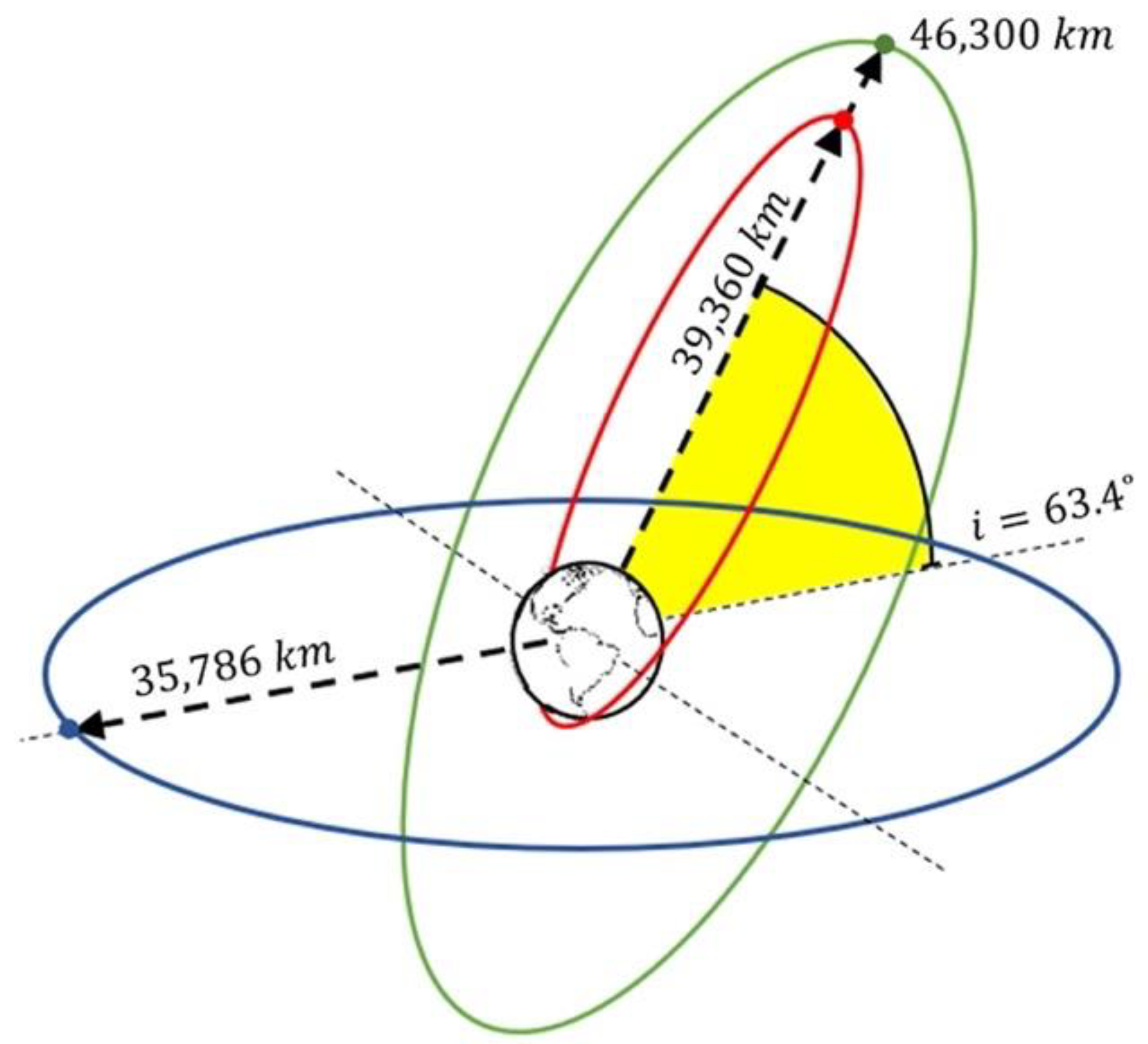
Figure 4.
(A) The simplest Molniya/GEO constellation to provide continuous global coverage with 2 Molniya over the poles. (B) Constellation ground tracks.
Figure 4.
(A) The simplest Molniya/GEO constellation to provide continuous global coverage with 2 Molniya over the poles. (B) Constellation ground tracks.

Figure 5.
Cross section radiance measure and respective VIIRS images for (A) Aurora Borealis core, taken 11:18 UTC 13 February 2019, (B) Aurora Borealis fine structure, taken 11:18 UTC 13 February 2019, (C) Aurora Australis from core to fine structure, taken 19:30 UTC 5 February 2019, (D) Night-time Lights of Europe, taken 01:06 UTC 3 February 2019. All data acquired from NASA LAADS DAAC.

Figure 6.
Radiance range comparison of the features that are desirable to radiometrically resolve and the resultant dynamic range required by a sensor to achieve this.
Figure 6.
Radiance range comparison of the features that are desirable to radiometrically resolve and the resultant dynamic range required by a sensor to achieve this.

Figure 7.
Cumulative global coverage from combined LEO instruments.

Figure 8.
GEO coverage from GOES-16, GOES-17, Meteosat-8, Meteosat-11 and Himawari-8 in the ±60° latitude band.
Figure 8.
GEO coverage from GOES-16, GOES-17, Meteosat-8, Meteosat-11 and Himawari-8 in the ±60° latitude band.
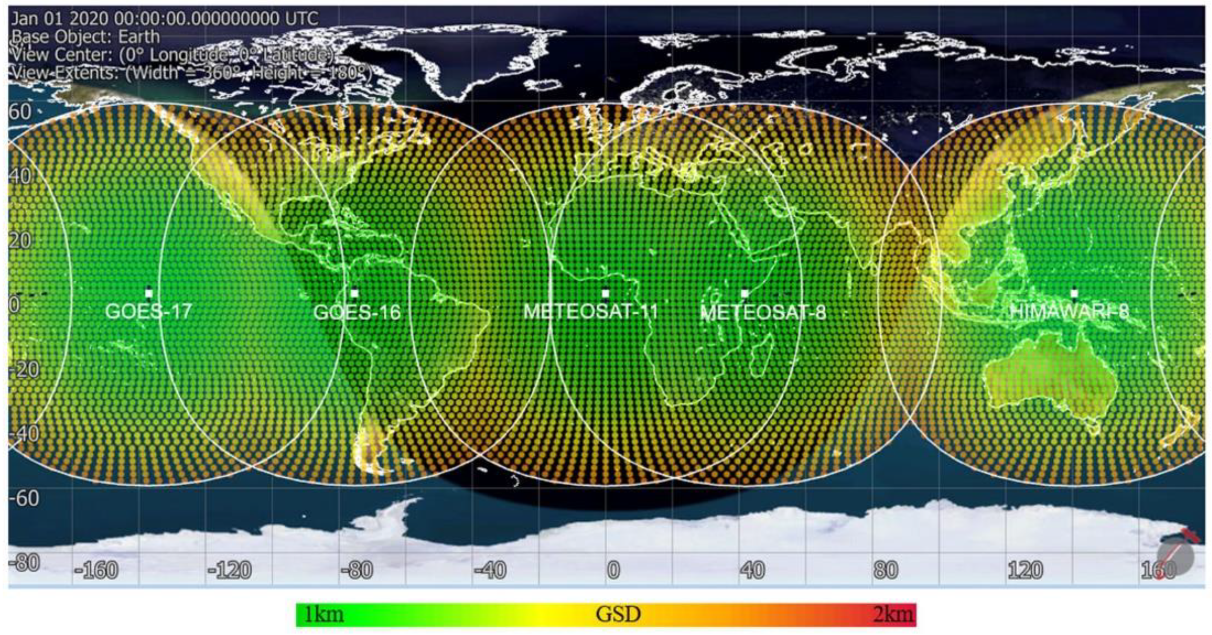
Figure 9.
Cumulative global coverage from combined LEO and GEO instruments.
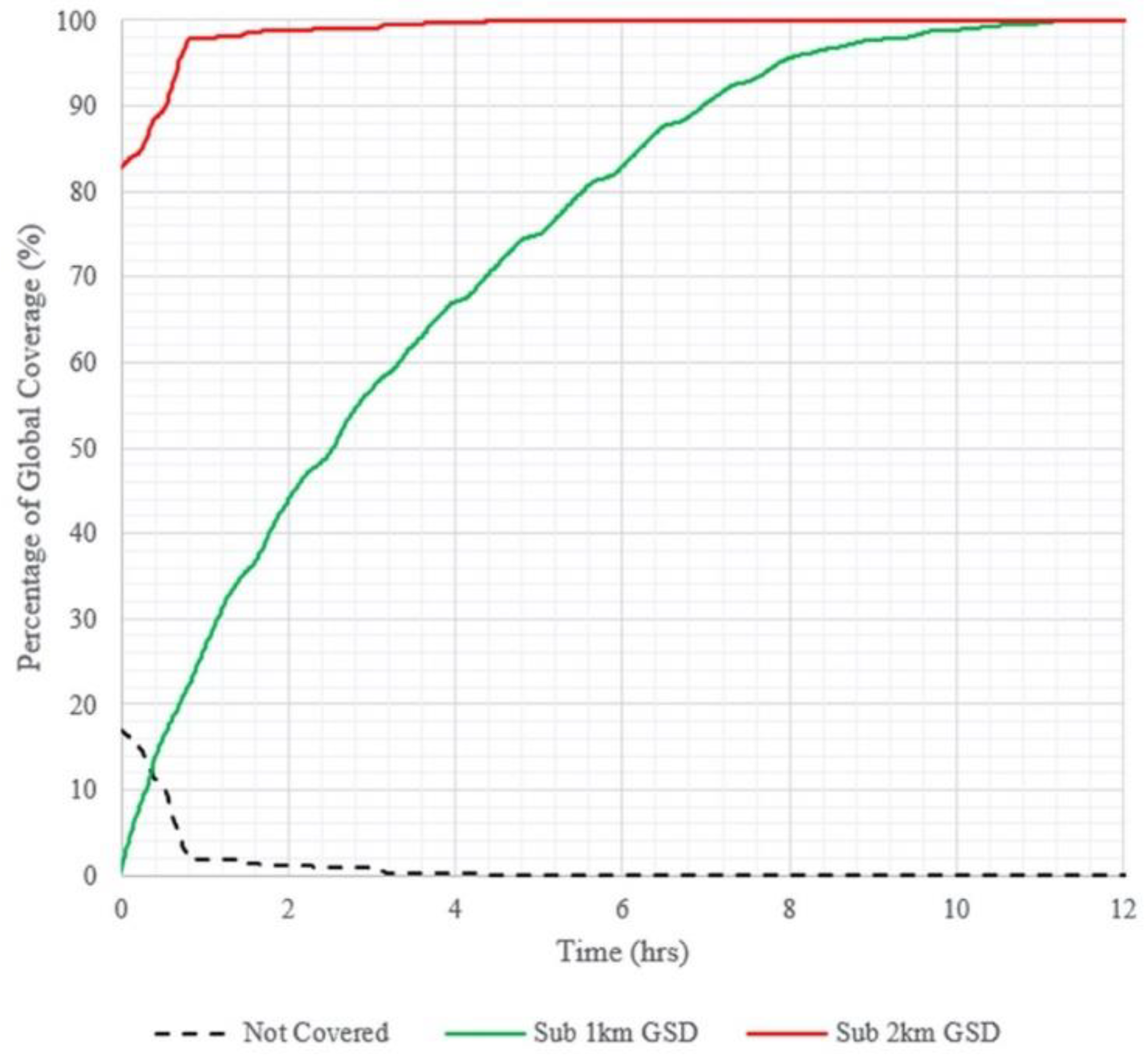
Figure 10.
Constellation formations (I) and global distribution of GSD (II) at the time of maximum distortion for the Nine (A), Eleven (B) and Thirteen (C) satellite cases.
Figure 10.
Constellation formations (I) and global distribution of GSD (II) at the time of maximum distortion for the Nine (A), Eleven (B) and Thirteen (C) satellite cases.
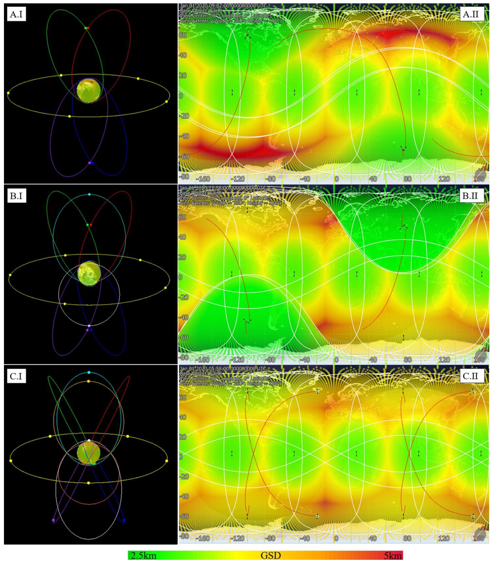
Figure 11.
Percentage of global coverage at varying degrees of resolution for the (A) Nine, (B) Eleven, and (C) Thirteen satellite cases.
Figure 11.
Percentage of global coverage at varying degrees of resolution for the (A) Nine, (B) Eleven, and (C) Thirteen satellite cases.

Figure 12.
BRDF sampling quality showing the number of view angles within 10° of the SPP for (A) nine, (B) eleven, (C) thirteen satellite architectures.
Figure 12.
BRDF sampling quality showing the number of view angles within 10° of the SPP for (A) nine, (B) eleven, (C) thirteen satellite architectures.
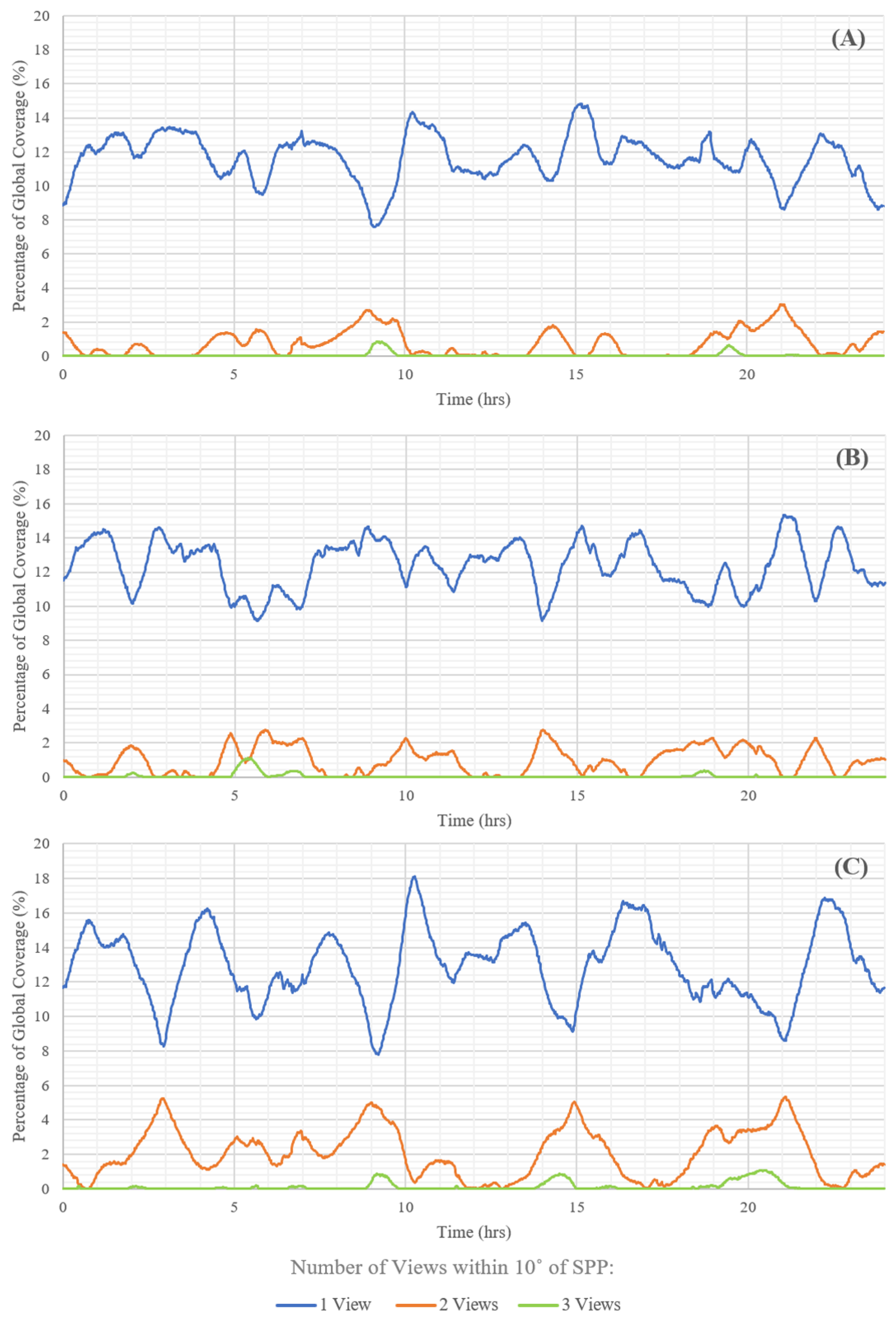
Figure 13.
Ground Sample Distance as a function of angular distance from satellite nadir for 4K and 8K sensors at GEO altitude.
Figure 13.
Ground Sample Distance as a function of angular distance from satellite nadir for 4K and 8K sensors at GEO altitude.
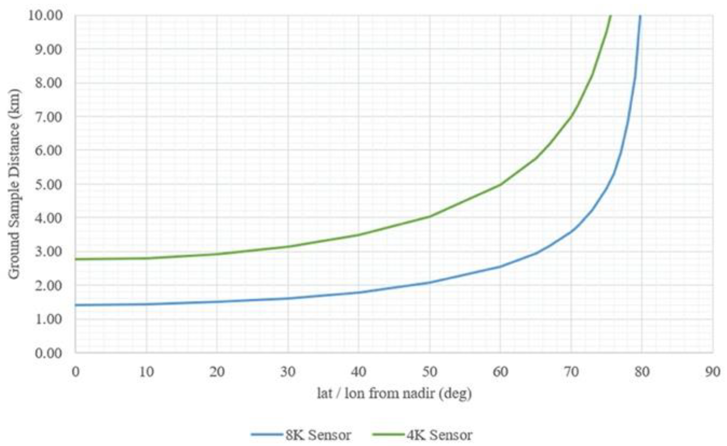
Figure 14.
Sub 2 km resolution overlap of Meteosat-11, Meteosat-8, Himawari-8, GOES-16 and GOES-17, defining stereoscopic availability.
Figure 14.
Sub 2 km resolution overlap of Meteosat-11, Meteosat-8, Himawari-8, GOES-16 and GOES-17, defining stereoscopic availability.

Figure 15.
Percentage of global stereo coverage being viewed by two, three, four, five or six angles for increasing numbers of equally spaced GEO observers.
Figure 15.
Percentage of global stereo coverage being viewed by two, three, four, five or six angles for increasing numbers of equally spaced GEO observers.
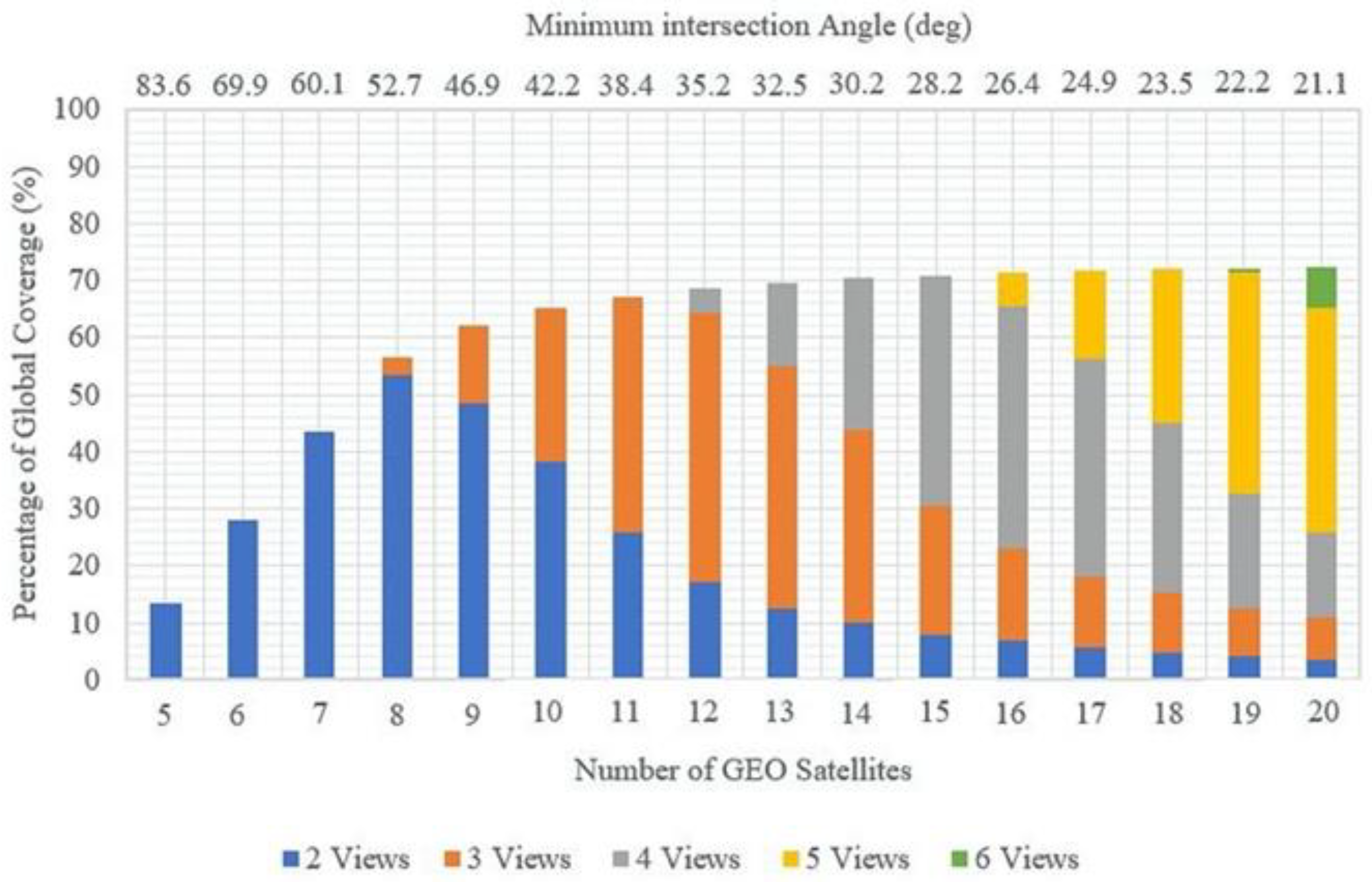
Figure 16.
Representational renderings of the Molniya 20° FOV at various times into the 12-h orbit.
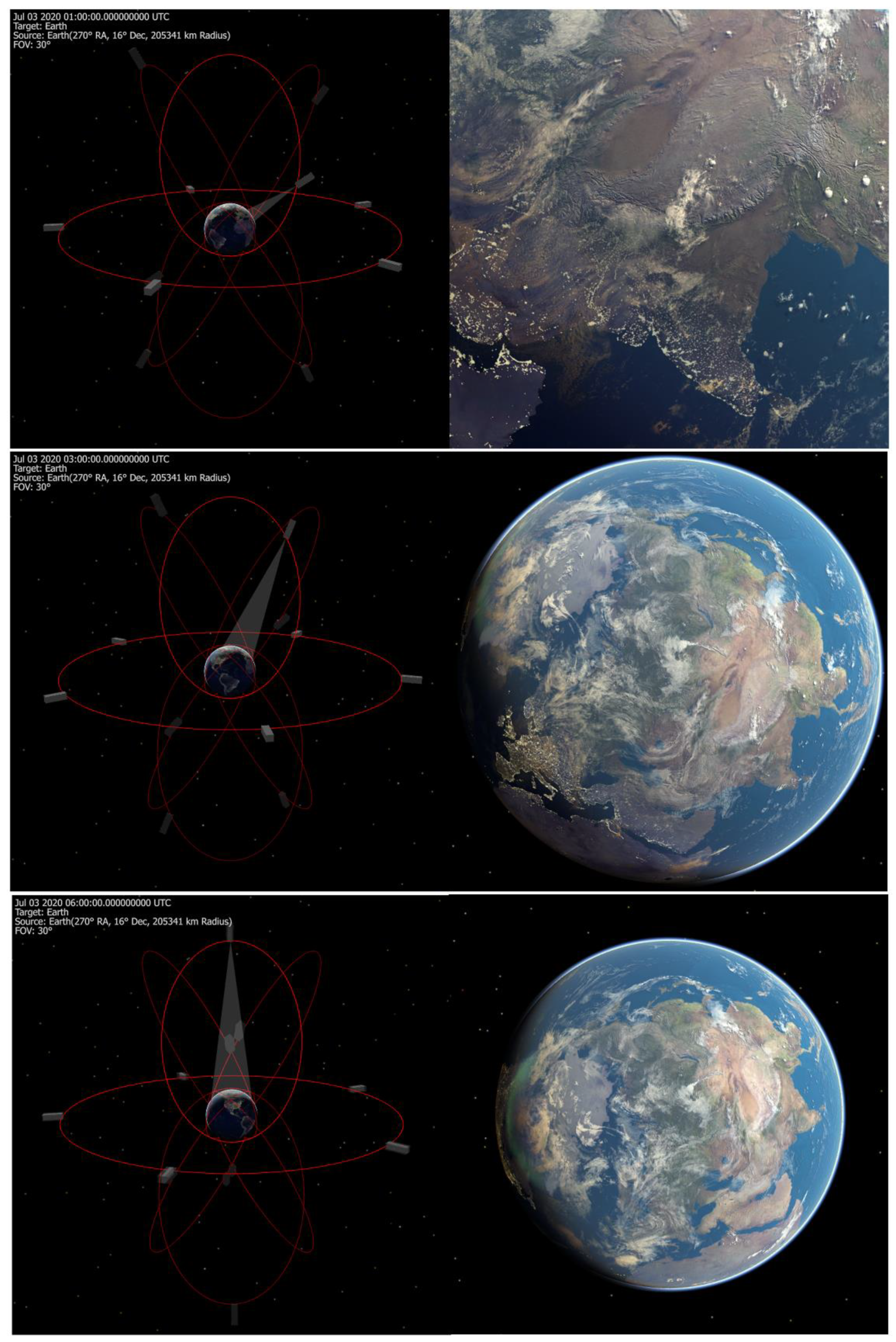
Figure 17.
Representational renderings of the GEO 18° FOV at various times into the 24-h orbit.
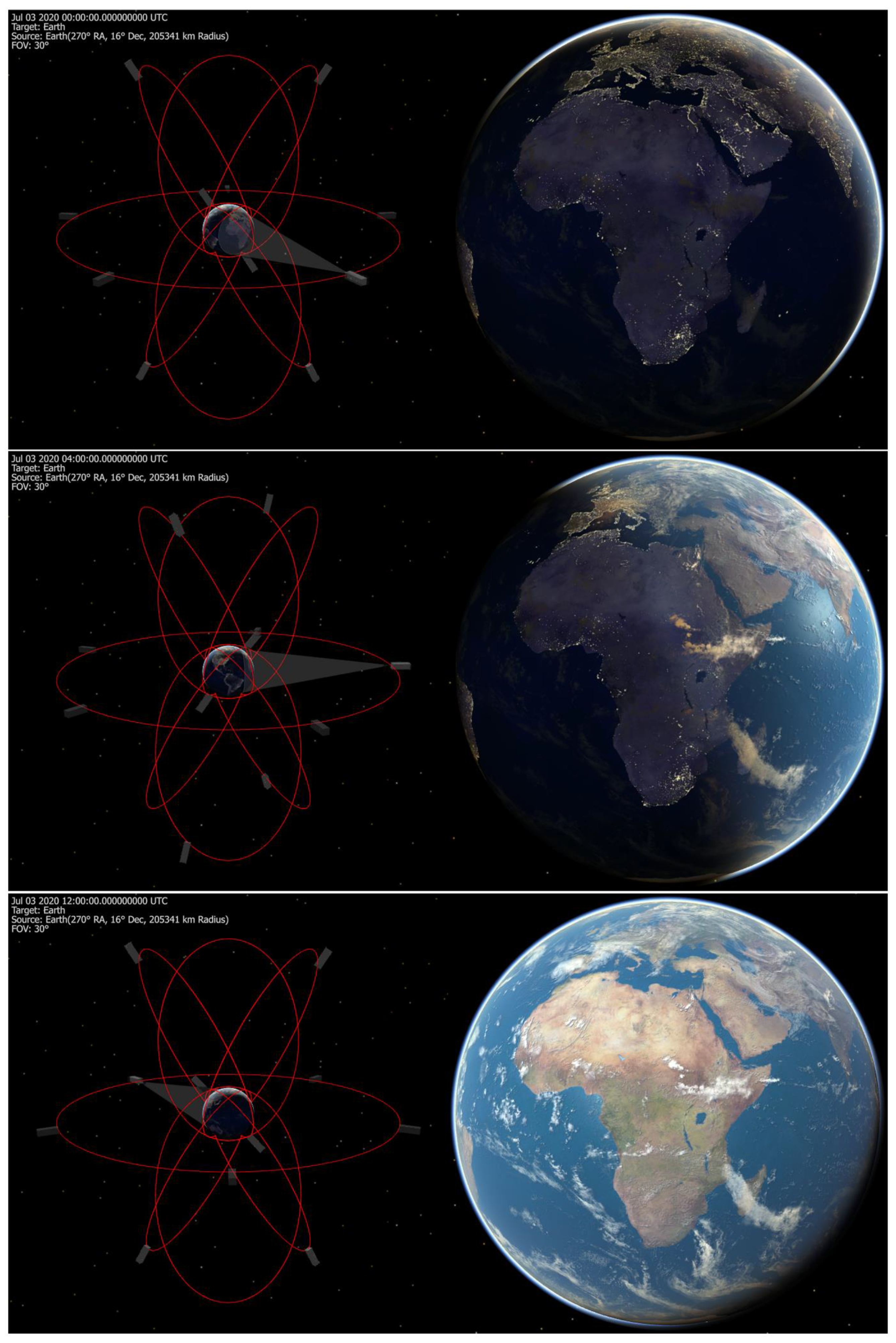
Figure 18.
Average integral flux of trapped electrons in LEO, GEO and Molniya orbit.

Figure 19.
Average integral flux of trapped protons in LEO, GEO and Molniya orbit.

Figure 20.
Average integral flux of solar protons in LEO, GEO and Molniya orbit.
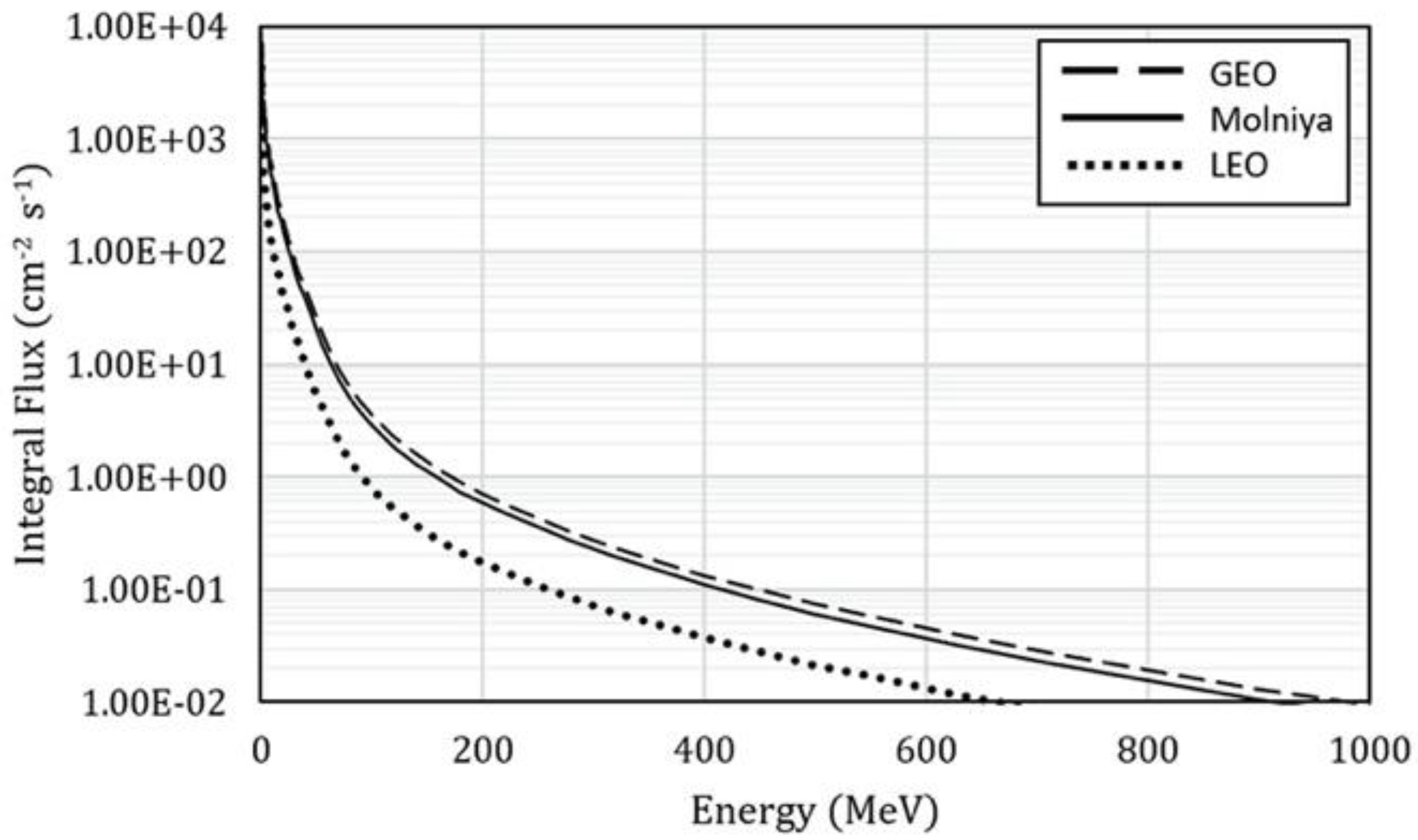
Figure 21.
Estimated Lifetime (time to receive TID of 30 krad) in GEO and Molniya as a function of shielding thickness and the equivalent mass for the 10 × 10 × 30 cm surface area of a 3U CubeSat.
Figure 21.
Estimated Lifetime (time to receive TID of 30 krad) in GEO and Molniya as a function of shielding thickness and the equivalent mass for the 10 × 10 × 30 cm surface area of a 3U CubeSat.
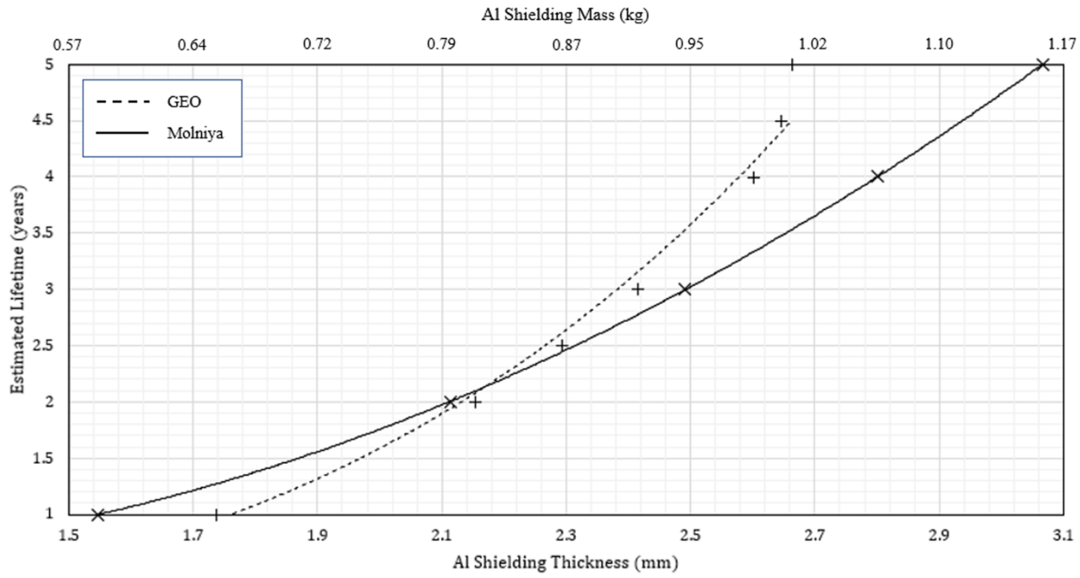

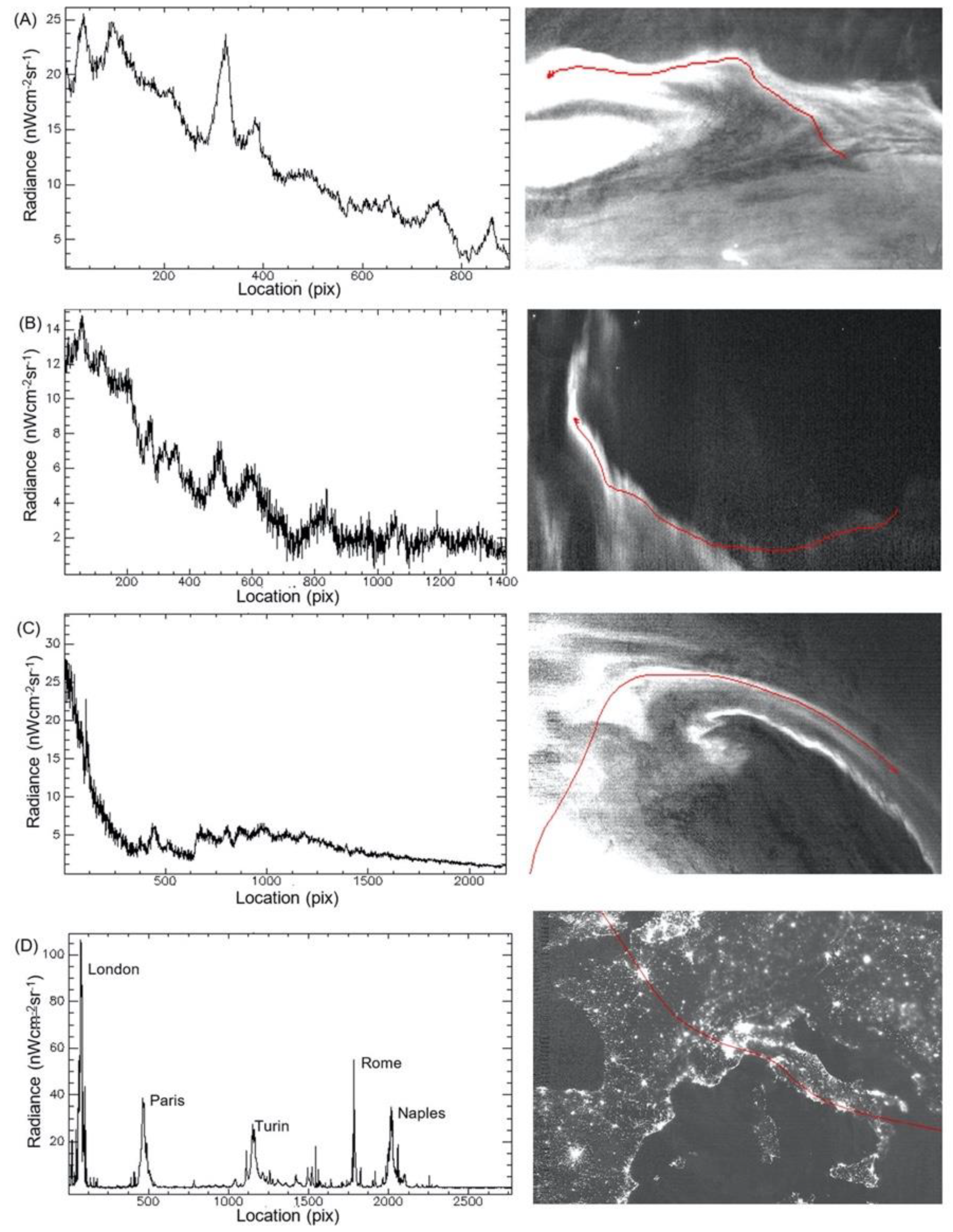
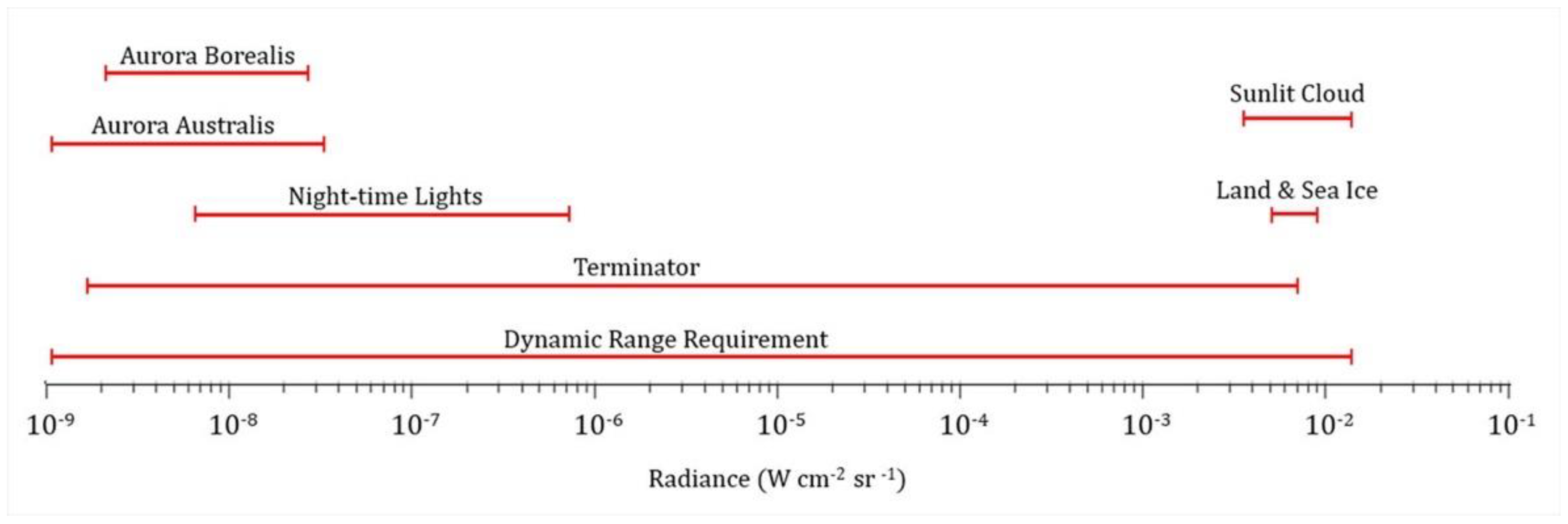
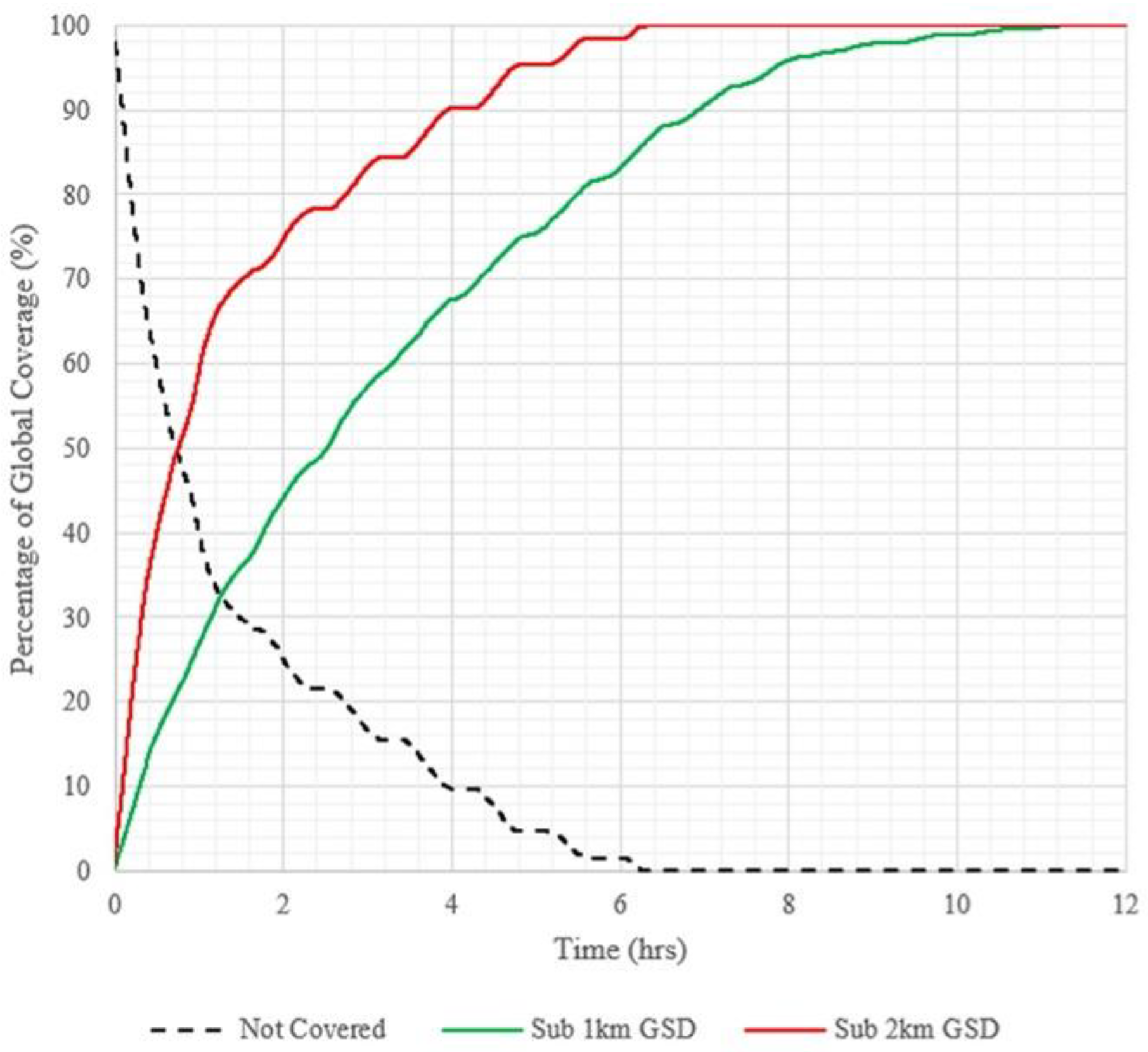
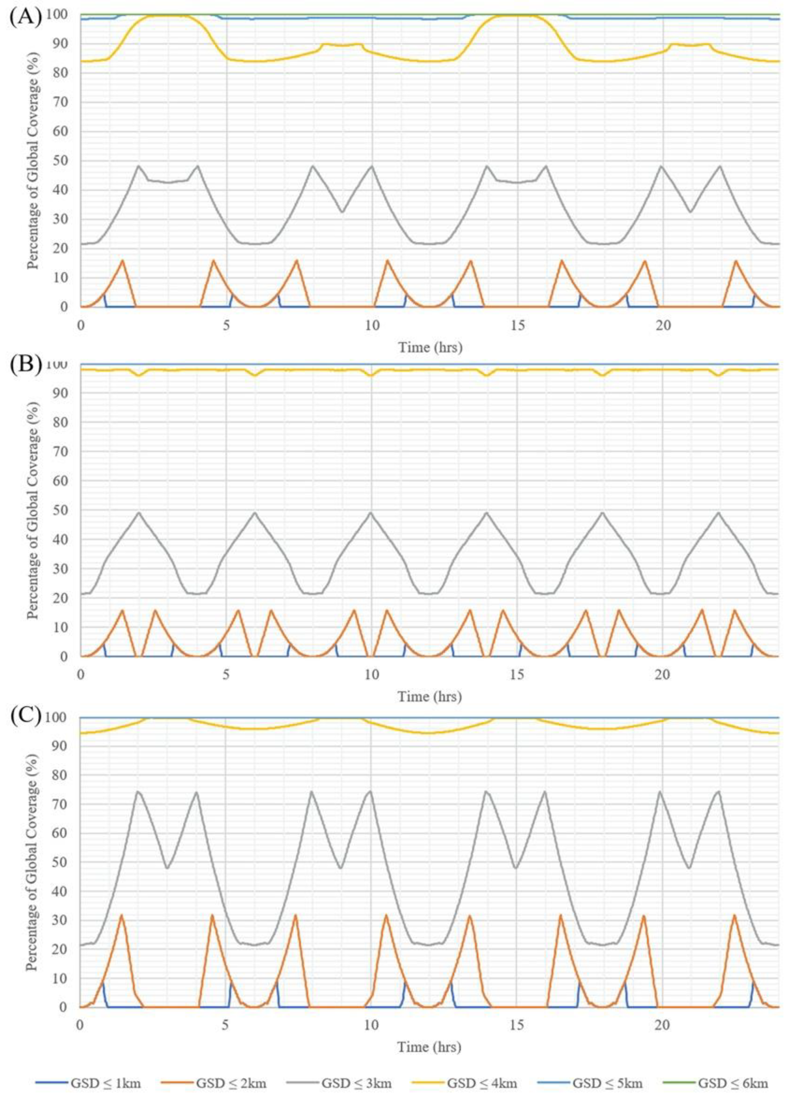
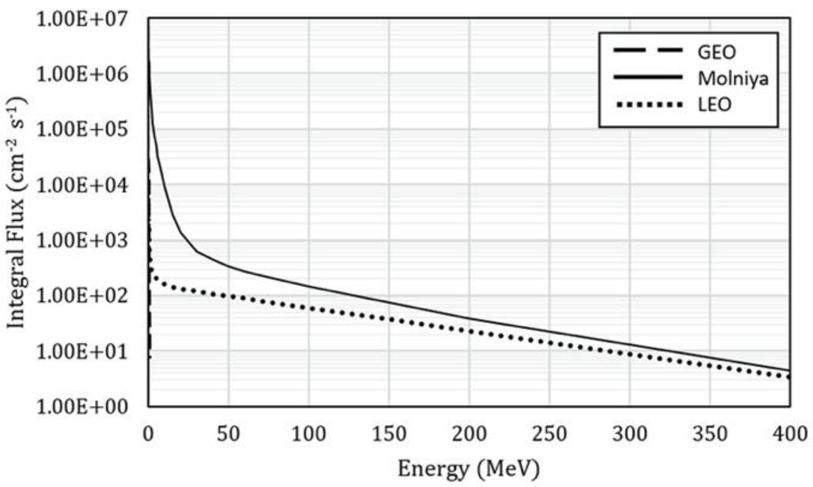
Table 1.
Deduced camera parameters and resultant Ground Separation Distance/Field of View (GSD/FOV) at the Earth’s surface.
Table 1.
Deduced camera parameters and resultant Ground Separation Distance/Field of View (GSD/FOV) at the Earth’s surface.
| Molniya | GEO | Tundra | |
|---|---|---|---|
| Apogee Altitude (km) | 39,850 | 35,788 | 46,300 |
| Crossing Point Altitude (km) | 31,472 | N/A | 38,339 |
| X Pixels | 4096 | 4 096 | 4096 |
| Pixel Size (μm) | 9.60 | 7.75 | 10 |
| Sensor Horizontal (mm) | 19.66 | 15.87 | 20.48 |
| Focal Length (mm) | 111.55 | 100.18 | 129.31 |
| Aperture (mm) | 55.77 | 50.09 | 64.80 |
| f/# | 2 | 2 | 2 |
| GSD from Apogee (km) | 3.43 | 2.77 | 3.58 |
| GSD from Crossing Point (km) | 2.71 | N/A | 2.97 |
| FOV (deg) | 20 | 18 | 18 |
| FOV from Apogee (km) | 16,303 | 13,357 | 14,666 |
Table 2.
Sensor specifications of 4K sensors and their calculated optics parameters for a 20° FOV in Molniya orbit. The AC-4 Megapixel sensor (Aptina MT9D131 [26]) is also included for comparison.
Table 2.
Sensor specifications of 4K sensors and their calculated optics parameters for a 20° FOV in Molniya orbit. The AC-4 Megapixel sensor (Aptina MT9D131 [26]) is also included for comparison.
| IDS UI-3590CP-C | Lumenera Lt1245R | Kodak KA1-11002 | MT9F002 | KAF-16801 | KAI-16070 | Aptina MT9D131 (AC-4) | |
|---|---|---|---|---|---|---|---|
| Ref | [44] | [45] | [46] | [47] | [48] | [49] | [43] |
| X Pixels | 4912 | 4112 | 4032 | 4384 | 4096 | 4864 | 1600 |
| Y Pixels | 3684 | 3008 | 2688 | 3288 | 4096 | 3232 | 1200 |
| Pixel Size (μm) | 1.25 | 3.45 | 9 | 1.4 | 9 | 7.4 | 2.8 |
| Sensor Horizontal (mm) | 3.07 | 7.09 | 18.14 | 3.07 | 18.43 | 18.00 | 2.24 |
| Sensor Vertical (mm) | 2.30 | 3.75 | 12.10 | 2.30 | 18.43 | 11.96 | 1.68 |
| Focal Length (mm) | 17.41 | 40.23 | 102.90 | 17.40 | 104.53 | 102.06 | 12.70 |
| Aperture (mm) | 8.71 | 20.11 | 51.45 | 8.70 | 52.27 | 51.03 | 6.35 |
| f/# | 2 | 2 | 2 | 2 | 2 | 2 | 2 |
| GSD at Apogee (km) | 2.86 | 3.42 | 3.49 | 3.21 | 3.43 | 2.89 | 8.78 |
| GSD at Crossing Point (km) | 2.26 | 2.70 | 2.75 | 2.53 | 2.71 | 2.28 | 6.94 |
| Horizontal FOV (km) | 16,303 | 16,303 | 16,303 | 16,303 | 16,303 | 16,303 | 16,303 |
| Vertical FOV (km) | 12,227 | 11,925 | 10,868 | 12,227 | 16,303 | 10,833 | 12,227 |
Table 3.
Sensor specifications of 4K sensors and their calculated optics parameters for an 18° FOV in geostationary orbit. The AC-4 Megapixel sensor (Aptina MT9D131 [26]) is also included for comparison.
Table 3.
Sensor specifications of 4K sensors and their calculated optics parameters for an 18° FOV in geostationary orbit. The AC-4 Megapixel sensor (Aptina MT9D131 [26]) is also included for comparison.
| IDS UI-3590CP-C | Lumenera Lt1245R | Kodak KA1-11002 | MT9F002 | KAF-16801 | KAI-16070 | Aptina MT9D131 (AC-4) | |
|---|---|---|---|---|---|---|---|
| Ref | [44] | [45] | [46] | [47] | [48] | [49] | [43] |
| X Pixels | 4912 | 4112 | 4032 | 4384 | 4096 | 4864 | 1600 |
| Y Pixels | 3684 | 3008 | 2688 | 3288 | 4096 | 3232 | 1200 |
| Pixel Size (μm) | 1.25 | 3.45 | 9 | 1.4 | 9 | 7.4 | 2.8 |
| Sensor Horizontal (mm) | 3.07 | 7.09 | 18.14 | 3.07 | 18.43 | 18.00 | 2.24 |
| Sensor Vertical (mm) | 2.30 | 5.19 | 12.10 | 2.30 | 18.43 | 11.96 | 1.68 |
| Focal Length (mm) | 19.38 | 44.78 | 114.56 | 19.38 | 116.38 | 113.63 | 14.14 |
| Aperture (mm) | 9.69 | 22.39 | 57.28 | 9.69 | 58.19 | 56.81 | 7.07 |
| f/# | 2 | 2 | 2 | 2 | 2 | 2 | 2 |
| GSD (km) | 2.31 | 2.76 | 2.81 | 2.59 | 2.77 | 2.33 | 7.09 |
| Horizontal FOV (km) | 13,357 | 13,357 | 13,357 | 13,357 | 13,357 | 13,357 | 13,357 |
| Vertical FOV (km) | 10,018 | 9771 | 8905 | 10,018 | 13,357 | 8875 | 10,018 |
Table 4.
Sensor specifications of 4K sensors and their calculated optics parameters for a 18° FOV in Tundra orbit. The AC-4 Megapixel sensor (Aptina MT9D131 [26]) is also included for comparison.
Table 4.
Sensor specifications of 4K sensors and their calculated optics parameters for a 18° FOV in Tundra orbit. The AC-4 Megapixel sensor (Aptina MT9D131 [26]) is also included for comparison.
| IDS UI-3590CP-C | Lumenera Lt1245R | Kodak KA1-11002 | MT9F002 | KAF-16801 | KAI-16070 | Aptina MT9D131 (AC-4) | |
|---|---|---|---|---|---|---|---|
| Ref | [44] | [45] | [46] | [47] | [48] | [49] | [43] |
| X Pixels | 4912 | 4112 | 4032 | 4384 | 4096 | 4864 | 1600 |
| Y Pixels | 3684 | 3008 | 2688 | 3288 | 4096 | 3232 | 1200 |
| Pixel Size (μm) | 1.25 | 3.45 | 9 | 1.4 | 9 | 7.4 | 2.8 |
| Sensor Horizontal (mm) | 3.07 | 7.09 | 18.14 | 3.07 | 18.43 | 18.00 | 2.24 |
| Sensor Vertical (mm) | 2.30 | 3.75 | 12.10 | 2.30 | 18.43 | 11.96 | 1.68 |
| Focal Length (mm) | 19.38 | 44.78 | 114.56 | 19.38 | 116.38 | 113.63 | 14.14 |
| Aperture (mm) | 9.69 | 22.39 | 57.28 | 9.69 | 58.19 | 56.81 | 7.07 |
| f/# | 2 | 2 | 2 | 2 | 2 | 2 | 2 |
| GSD at Apogee (km) | 2.99 | 3.57 | 3.64 | 3.35 | 3.58 | 3.02 | 9.17 |
| GSD at Crossing Point (km) | 2.47 | 2.95 | 3.01 | 2.77 | 2.97 | 2.50 | 7.59 |
| Horizontal FOV (km) | 14,666 | 14,666 | 14,666 | 14,666 | 14,666 | 14,666 | 14,666 |
| Vertical FOV (km) | 11,000 | 10,729 | 9778 | 11,000 | 14,666 | 9745 | 11,000 |
Table 5.
LEO visible band instruments to provide integrated global coverage.
| Instrument | LEO Orbiter | Spatial Resolution Nadir (km) | Swath Width (km) | Global Coverage | Ref |
|---|---|---|---|---|---|
| MODIS | TERRA/AQUA | 1.000 | 2330 | 1–2 Days | [56] |
| VIIRS | NOAA 20/Suomi NPP | 0.742 | 3000 | Daily | [19,57] |
| OLCI | Sentinel-3A/Sentinel-3B | 0.300 | 1270 | 0.9 Days | [58] |
| AVHRR | MetOp-A/MetOp-B/MetOp-C | 1.100 | 2894 | Twice Daily | [59] |
Table 6.
Average global percentage of multi-view coverage.
| Constellation Size | No. Molniya Satellites | No. GEO Satellites | Average Percentage of Globe in View of at Least: | |||||||
|---|---|---|---|---|---|---|---|---|---|---|
| 1 Sat | 2 Sats | 3 Sats | 4 Sats | 5 Sats | 6 Sats | 7 Sats | 8 Sats | |||
| 9 | 4 | 5 | 99.98 | 99.14 | 87.67 | 32.09 | 3.29 | 0.00 | 0.00 | 0.00 |
| 10 | 4 | 6 | 100 | 99.22 | 94.21 | 59.67 | 11.50 | 0.00 | 0.00 | 0.00 |
| 11 | 6 | 5 | 100 | 99.99 | 96.30 | 64.63 | 15.37 | 1.07 | 0.00 | 0.00 |
| 12 | 6 | 6 | 100 | 99.99 | 98.07 | 81.58 | 36.34 | 3.75 | 0.00 | 0.00 |
| 13 | 8 | 5 | 100 | 100 | 98.23 | 83.92 | 38.30 | 10.67 | 1.06 | 0.00 |
| 14 | 8 | 6 | 100 | 100 | 99.25 | 91.17 | 60.98 | 19.07 | 4.06 | 0.00 |
Table 7.
Summary of quality of coverage for varying GEO + Molniya constellation architectures.
| Constellation Size | 9 | 10 | 11 | 12 | 13 | 14 |
|---|---|---|---|---|---|---|
| No Molniya Satellites | 4 | 4 | 6 | 6 | 8 | 8 |
| No GEO Satellites | 5 | 6 | 5 | 6 | 5 | 6 |
| Maximum GSD (km) | 5.760 | 5.631 | 4.738 | 4.622 | 4.710 | 4.429 |
| Average GSD (km) | 3.245 | 3.204 | 3.114 | 3.077 | 3.017 | 2.984 |
| Standard Deviation (km) | 0.145 | 0.138 | 0.098 | 0.096 | 0.202 | 0.195 |
| Average Coverage of Instantaneous Multiple BRDF Sampling (%) | 0.764 | 0.868 | 1.013 | 1.100 | 2.192 | 2.346 |
| Standard Deviation (%) | 0.811 | 0.817 | 0.839 | 0.707 | 1.562 | 1.481 |
Publisher’s Note: MDPI stays neutral with regard to jurisdictional claims in published maps and institutional affiliations. |
© 2021 by the authors. Licensee MDPI, Basel, Switzerland. This article is an open access article distributed under the terms and conditions of the Creative Commons Attribution (CC BY) license (http://creativecommons.org/licenses/by/4.0/).
Share and Cite
MDPI and ACS Style
Cullingworth, C.; Muller, J.-P. Contemporaneous Monitoring of the Whole Dynamic Earth System from Space, Part I: System Simulation Study Using GEO and Molniya Orbits. Remote Sens. 2021, 13, 878. https://doi.org/10.3390/rs13050878
AMA Style
Cullingworth C, Muller J-P. Contemporaneous Monitoring of the Whole Dynamic Earth System from Space, Part I: System Simulation Study Using GEO and Molniya Orbits. Remote Sensing. 2021; 13(5):878. https://doi.org/10.3390/rs13050878
Chicago/Turabian StyleCullingworth, Christopher, and Jan-Peter Muller. 2021. "Contemporaneous Monitoring of the Whole Dynamic Earth System from Space, Part I: System Simulation Study Using GEO and Molniya Orbits" Remote Sensing 13, no. 5: 878. https://doi.org/10.3390/rs13050878
Note that from the first issue of 2016, this journal uses article numbers instead of page numbers. See further details here.