Validation of GOSAT and OCO-2 against In Situ Aircraft Measurements and Comparison with CarbonTracker and GEOS-Chem over Qinhuangdao, China

Abstract

Carbon dioxide (CO₂) is the most important greenhouse gas and several satellites have been launched to monitor the atmospheric CO₂ at regional and global scales. Evaluation of the measurements obtained from these satellites against accurate and precise instruments is crucial. In this work, aircraft measurements of CO₂ were carried out over Qinhuangdao, China (39.9354°N, 119.6005°E), on 14, 16, and 19 March 2019 to validate the Greenhous gases Observing SATellite (GOSAT) and the Orbiting Carbon Observatory 2 (OCO-2) CO₂ retrievals. The airborne in situ instruments were mounted on a research aircraft and the measurements were carried out between the altitudes of ~0.5 and 8.0 km to obtain the vertical profiles of CO₂. The profiles captured a decrease in CO₂ concentration from the surface to maximum altitude. Moreover, the vertical profiles from GEOS-Chem and the National Oceanic and Atmospheric Administration (NOAA) CarbonTracker were also compared with in situ and satellite datasets. The satellite and the model datasets captured the vertical structure of CO₂ when compared with in situ measurements, which showed good agreement among the datasets. The dry-air column-averaged CO₂ mole fractions (XCO₂) retrieved from OCO-2 and GOSAT showed biases of 1.33 ppm (0.32%) and −1.70 ppm (−0.41%), respectively, relative to the XCO₂ derived from in situ measurements.

1. Introduction

Atmospheric carbon dioxide (CO₂) is the most important greenhouse gas and its concentration has increased globally from 280 ppm before industrialization to over 410 ppm at present [1,2,3]. The global average temperature increased by 0.85 °C from 1880 to 2012 [4] and the increased atmospheric CO₂ levels related to anthropogenic activities have significantly contributed to this because they absorb and emit radiant energy within the thermal infrared range [5]. The precise prediction of the atmospheric CO₂ concentration and its influence on climate change requires accurate quantification of the distribution and variability of CO₂ sources and sinks [6,7]. Ground stations and tall towers with flask sampling, such as stations within the Global Atmospheric Watch (GAW) network [8], can measure the atmospheric CO₂ concentration with high precision and can provide the mole fractions of atmospheric CO₂ at regional and global scales. However, these measurements are representative of the lower atmosphere and do not provide information about the upper atmosphere [9]. The spatial coverage of GAW network stations is limited and their measurements are insufficient for total-column CO₂ analysis, producing uncertainties in the vertical as well as the horizontal direction. Moreover, a comprehensive network of ground-based, sun-viewing, near-infrared Fourier transform spectrometers known as the Total Carbon Column Observing Network (TCCON) accurately measures the concentrations of various greenhouse gases including CO₂, CO, CH₄, and N₂O [10,11]. Under clear atmospheric conditions, TCCON measures the CO₂ concentration with a precision of 0.25% [12]. However, TCCON sites are not sufficient for accurately measuring the amount of atmospheric CO₂ at regional and global scales due to their uneven distribution and limited spatial coverage [13,14,15].

Satellite-based measurements provide the most effective way to monitor the atmospheric CO₂ at regional and global scales with high spatiotemporal resolutions. At present, several satellites are dedicatedly monitoring the atmospheric CO₂ concentrations, such as OCO-3 [16], GOSAT-2 [17], TanSat [18,19], OCO-2 [20,21], and GOSAT [22]. These satellites calculate the average atmospheric CO₂ concentrations in the path of sunlight reflected by the surface through spectrometers carried onboard. OCO-2 and GOSAT use the same observational approach. For instance, both of them measure the CO₂ optical depth with bands centered around 2.0 and 1.6 μm and determine O₂ optical depth with band A, which is centered around 0.76 μm. The information retrieved from these three bands is combined to compute the column-averaged CO₂ dry-air mole fraction (XCO₂). The satellite data are vulnerable to aerosols and clouds and many of the data become unusable due to the presence of aerosol and cloud content in the measurements [23,24]. GOSAT contains a dedicated instrument known as Clouds and Aerosol Imager (CAI) to detect the clouds and aerosols. The measurements obtained from these satellites need to be evaluated against precise airborne and ground-based measurements [25,26]. Measurements from ground-based instruments such as TCCON have good accuracy and are often used to validate the satellite retrievals [27,28,29,30]. Though the airborne measurements are carried out less frequently, they provide precise observations with which to understand the vertical distribution of CO₂. The airborne data from the Comprehensive Observation Network for Trace gases by AIrLiner (CONTRAIL) project [31], HIAPER Pole-to-Pole Observation (HIPPO) project [32], and NOAA Earth System Research Laboratory (ESRL) greenhouse gas reference network aircraft [33] have been used for the validation of various satellites. The airborne measurements collected by the Alpha Jet Atmospheric Experiment (AJAX) have been used to compare with the vertical profiles of GOSAT [34].

China has accounted for 30% of the overall growth in global CO₂ emissions over the past 15 years [35]. This increment in the concentration of atmospheric CO₂ is mainly due to the rapid economic growth, combustion of fossil fuels, and cement production [36]. East China is a densely populated region and an economic growth engine that has a significant contribution to the increased levels of atmospheric CO₂. Under the United Nations Framework Convention on Climate Change (UNFCCC) 2015 Paris Climate Agreement, China has pledged a reduction in CO₂ emissions per unit GDP by 60–65% relative to 2005 levels, and peak carbon emissions overall, by 2030 [37]. Monitoring of the CO₂ reduction progress and evaluation of how well specific policies are working is hindered by large uncertainties in the existing data sources [38,39]. Several studies reported larger uncertainties in the satellite CO₂ retrievals over China, and these uncertainties were more significant in North and East China [3,5,40,41]. Thus, validation of satellite measurements of column CO₂ is very important for accurate monitoring of atmospheric CO₂. Moreover, validation of model measurements against accurate CO₂ profiles is also crucial, because the satellite retrieval algorithms require a priori profiles which are generally based on models and in situ data. Lack of direct and independent airborne observations over China may produce a larger bias in the satellite results. In this paper, we report the in situ vertical profile measurements of CO₂ carried out using an aircraft over Qinhuangdao, China in March 2019. An Ultraportable Greenhouse Gas Analyzer (UGGA; model 915-0011; Los Gatos Research, San Jose, CA, USA) was installed on the aircraft to measure the vertical mole fraction of CO₂ at altitudes of 0.5–8.0 km. The details of the instrument, experimental site, flights, and the datasets used in this study are described in Section 2. The results, including the XCO₂ and vertical profile comparisons, are discussed in Section 3.

2. Materials and Methods

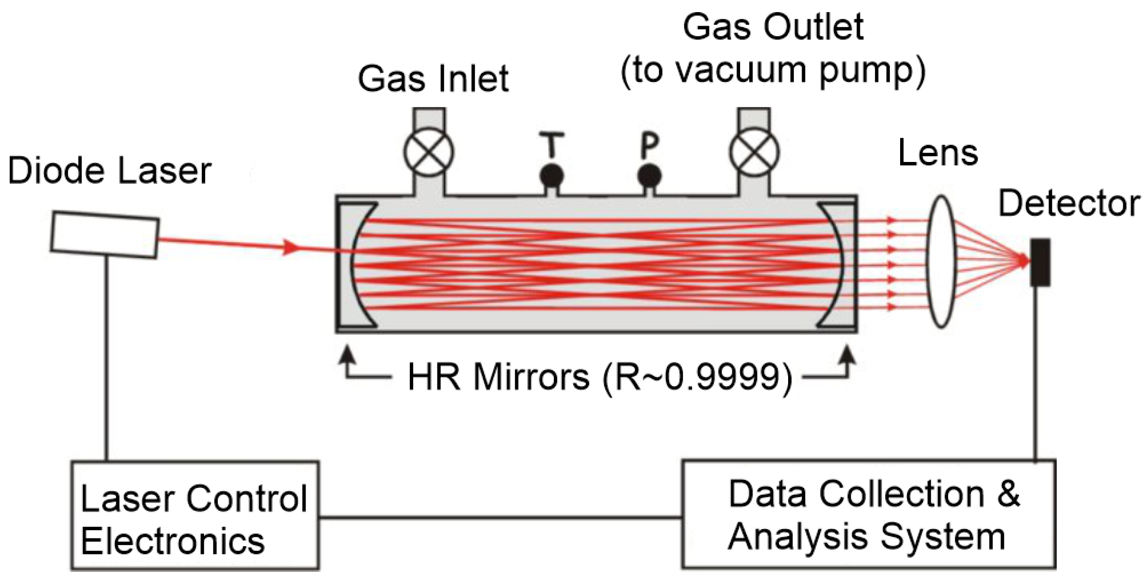
2.1. Aircraft Instrumentation

The aircraft used in this experiment was Yun-8, which was equipped with four turboprop engines mounted under the leading edges of non-swept wings. The cruise and the maximum speeds of the aircraft were 550 and 660 km h⁻¹, respectively. The Aircraft Integrated Meteorological Measurement System (AIMMS-20AG) was installed on the aircraft to measure the temperature, humidity, and wind speed. Moreover, the geolocation information, including longitude, latitude, the height of the aircraft, and the ambient pressure, can also be measured by AIMMS-20AG. The pressure, temperature, and humidity measured during the flight on each observation day are shown in Figure A2, Figure A3 and Figure A4, respectively. A commercial instrument, the Ultraportable Greenhouse Gas Analyzer (UGGA; model 915-0011; Los Gatos Research, San Jose, CA, USA), was installed in a non-sealed cabin of the aircraft. A small hole was drilled into the cabin wall and a ¼-inch Teflon pipe was used to connect the UGGA with the external atmosphere. To avoid the interference of the aircraft engine exhaust, the sampling hole was in front of the engine. The UGGA uses a laser absorption technology known as the off-axis Integrated Cavity Output Spectroscopy (ICOS) to measure trace gas concentration in dry mole fraction with a high precision of <0.30 ppm for CO₂ and <2 ppb for CH₄ (UGGA user manual; model 915-0011; Los Gatos Research, San Jose, CA, USA). The off-axis ICOS uses a high-finesse optical cavity as an absorption cell. Unlike the conventional multi-pass arrangements, which are typically limited to path lengths less than two meters, an off-axis ICOS absorption cell effectively traps the laser photon so that, on average, they make thousands of passes before leaving the cell. As a result, the effective optical path length may be several thousand meters using high-reflectivity mirrors and thus the measured absorption of light after it passes through the optical cavity is significantly enhanced (UGGA user manual). The schematic diagram of the off-axis ICOS is shown in Figure 1. More details on the off-axis ICOS spectroscopy are given in previous studies [42,43].

The UGGA was calibrated with respect to the standard gas and within the error range recommended by the World Meteorological Organization (WMO) before take-off and after landing of each flight to ensure the accuracy of the measurements. Before the flight, the clocks of AIMMS-20AG, UGGA, and other instruments were adjusted and synchronized to the altitude and geolocation of the aircraft. The UGGA and the synchronous meteorology measurements were recorded every second and then smoothed with a 10-s running average to further reduce the error caused by the temporal mismatch. The instrument was not continuously calibrated against the standard gas during flight. The first-order uncertainty was calculated, and the maximum average of 1σ on each observation day was considered to be the precision of the instrument. The accuracy of the CO₂ in the standard gas was below 0.50 ppm.

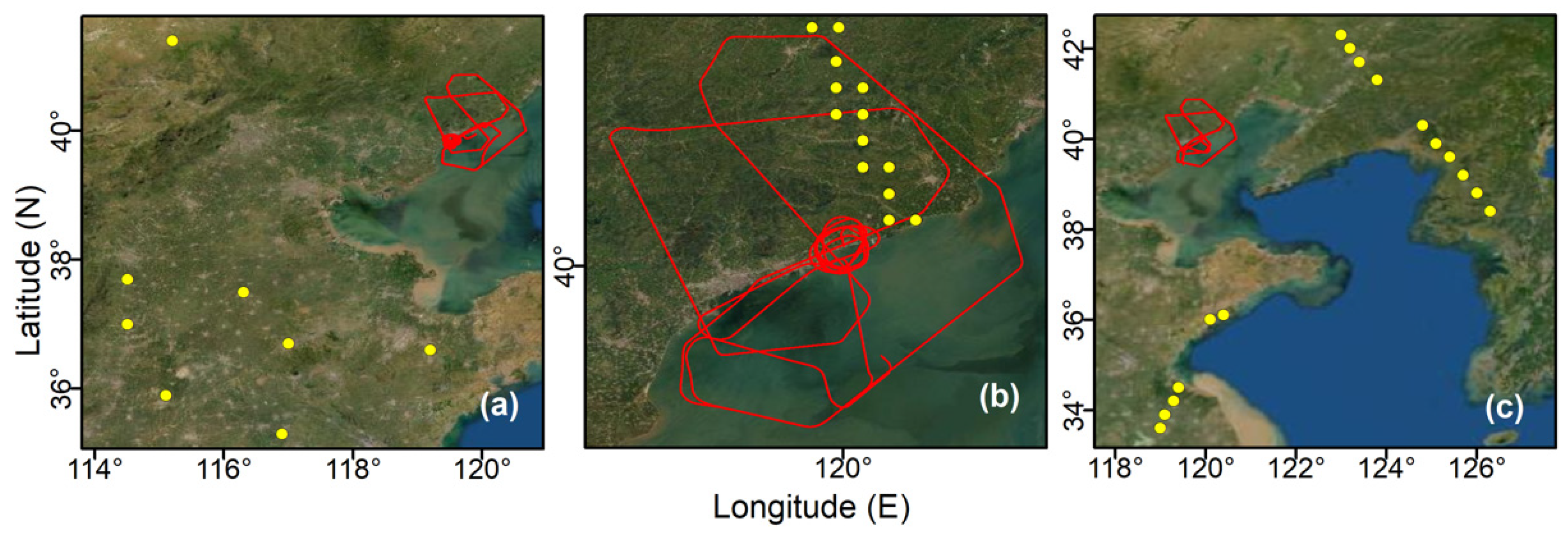
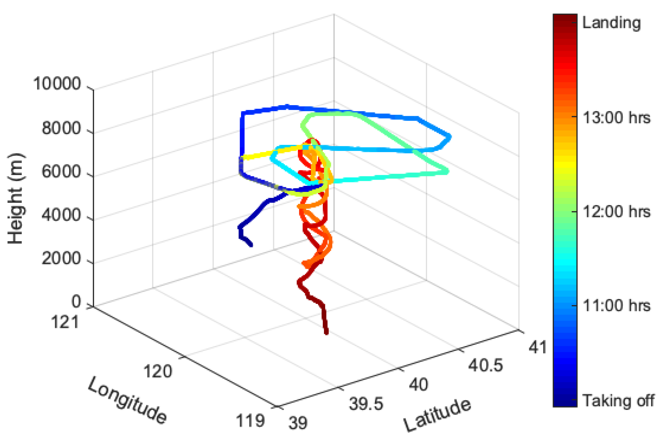
2.2. Experimental Site

The flights were carried out on 14, 16, and 19 March 2019 over Qinhuangdao, China (39.9354°N, 119.6005°E, ~5 m above sea level). Qinhuangdao is a port city and located in the northern Hebei province of China. It has a monsoon-influenced, humid, continental climate. Figure 2 shows the geolocation of the experimental site and paths of the flights. The experimental site contains a variety of land surfaces, including ocean, forest, towns, and mountains. The vertical profiles of CO₂ were obtained between 10:00 and 14:45 h CST (GMT +8). More detail about the flights is given in

Table 1. Details of flight on each day.

Date	Flight Time (CST)	Max Altitude (m)
14 March 2019	10:14:32–13:30:19	8000
16 March 2019	10:15:51–13:49:18	7000
19 March 2019	10:10:17–14:38:20	5000

.

The flight trajectory on 16 March is shown in Figure 3, and flight trajectories on 14 and 19 March are given in Figure A5. The plane took off around 10:15 h CST, climbed up quickly, and reached the maximum height. The aircraft started descending spirally at 12:45 h CST to the height of 2 km; then, it again climbed to the maximum height, descended again, and landed around 13:50 h CST. Keeping in view the sensitivity of the UGGA, the CO₂ measurements during ascent were rejected because of the rapid changes in the air pressure, and the measurements which were collected during descent were considered valid for the analysis. Moreover, the data collected below 0.5 km were also discarded due to the contamination of exhaust emission during the descent and slowing down of the aircraft. The weather was cloudy on 16 March in Qinhuangdao. More detail about the weather is given in the report released by the Meteorological Station of Qinhuangdao City (

Table 2. The weather report was released by the Meteorological Station of Qinhuangdao City on 14, 16, and 19 March 2019.

Date	Min Temperature	Max Temperature	Weather	Max Altitude (m)
14 March 2019	−1 °C	14 °C	Sunny	Northeast
16 March 2019	−1 °C	11 °C	Cloudy	North
19 March 2019	7 °C	15 °C	Cloudy	Southeast

).

2.3. Datasets

2.3.1. Satellite Datasets

In this paper, the datasets from two satellites, GOSAT and OCO-2, were used. GOSAT, the world’s first satellite dedicated to monitoring atmospheric CO₂ and CH₄, was launched on 23 January 2009 [22]. The sun-synchronous satellite with a repeat cycle of three days crosses the equator at approximately 13:00 local time and incorporates a Fourier transform spectrometer to measure three channels in the shortwave infrared (0.758–0.775, 1.56–1.72, and 1.92–2.08 μm) and one in the thermal infrared region (5.5–14.3 μm) [44]. The shortwave infrared bands retrieve the CO₂ column concentration and the thermal infrared band retrieves the vertical profiles of the CO₂ [45]. In this study, the ACOS/GOSAT XCO₂ version FP.9r Lite product was used. Previous studies have suggested that ACOS/GOSAT has better consistency than NIES/GOSAT [46].

Orbiting Carbon Observatory 2 (OCO-2) was launched by the National Aeronautics and Space Administration (NASA) on 2 July 2014 to monitor the CO₂ concentration at regional and global scales [20,21]. The near-polar, sun-synchronous satellite carries three high-resolution spectrometers that measure the near-infrared spectra of sunlight reflected off the Earth’s surface in three spectral regions centered at 0.765, 1.61, and 2.06 μm [29]. In this study, the OCO-2 XCO₂ version 10r Level 2 Lite product was used. These data were produced by the OCO-2 project at the Jet Propulsion Laboratory, California Institute of Technology, and obtained from the OCO-2 data archive maintained at the NASA Goddard Earth Science Data and Information Services Center.

2.3.2. Model Datasets

In this study, the datasets from two models, GEOS-Chem and CarbonTracker, were used. GEOS-Chem is a global three-dimensional (3D) chemical transport model that uses assimilated GEOS (Goddard Earth Observing System) meteorology from the NASA Global Modeling and Assimilation Office (GMAO) to drive the model. (Suntharalingam et al., 2004) [47] originally developed the GEOS-Chem CO₂ mode and (Nassar et al., 2010) [48] updated and improved the GEOS-Chem CO₂ simulation by adding CO₂ emissions from international shipping and aviation. The GEOS-Chem CO₂ simulation incorporates the monthly biomass burning data from Global Fire Emission Database (GFED) [49], cement production and fossil fuel data from Carbon Dioxide Information and Analysis Center (CDIAC) [50], terrestrial biosphere exchange from CASA biosphere model, and TransCom 3 project [51,52], and the ocean fluxes of CO₂ from Takahashi et al. [53]. In this study, the CO₂ was simulated using GEOS-Chem (version 12.9.3), with the prior CO₂ fluxes from fossil fuel combustion and cement production, biomass burning, biofuel burning, ocean exchanges, terrestrial exchanges, shipping, aviation, and chemical productions from the oxidation of carbon monoxide, as well as methane and non-methane volatile organic compounds. A similar model configuration has been used in a previous study to simulate the CO₂ over East Asia [54]. Moreover, the initial CO₂ concentration file, which was produced by a recent simulation, was provided by the GEOS-Chem CO₂ simulation group on request, and following their suggestion, the simulation was carried out from 1 January 2018 to 31 March 2019. The simulated CO₂ daily-averaged dataset included 47 vertical levels with a horizontal grid resolution of 2° × 2.5° latitude/longitude.

The CarbonTracker is a CO₂ data assimilation system developed by NOAA ESRL and it updates the surface fluxes and CO₂ distributions annually. It incorporates a two-way nested Transport Model 5 (TM5) offline atmospheric tracer transport model. The input CO₂ fluxes in the CarbonTracker include the fossil fuel emissions from Miller and Open-source Data Inventory for Anthropogenic CO₂ (ODIAC), biomass burning data from CASA-GFED, ocean fluxes of CO₂ from Takahashi et al. [53], and ocean inversion results [55], the assimilation of in-situ observations including tall towers, and flask sampled by the NOAA Cooperative Air Sampling Network, and the continuous measurements by partners. In this study, the CarbonTracker version CT-NRT.v2020-1 [56] was used which provides the CO₂ at 25 vertical levels with a temporal resolution of 3 h and spatial resolution of 2° × 3° latitude/longitude. More detail about the model is given at the CarbonTracker website (https://www.esrl.noaa.gov/gmd/ccgg/CT/, accessed on 9 February 2021).

3. Results and Discussion

3.1. Comparison of XCO₂ Products

The vertical profiles of CO₂ measured on the aircraft using UGGA on 14, 16, and 19 March 2019 are given in Figure 4. The maximum height covered by the aircraft was ~ 8 km on 16 March. The heights covered by the aircraft on each observation day are shown in Figure A1. To apply the smoothing correction, the aircraft vertical profiles must be extrapolated up to the whole atmosphere. To that end, we extrapolated the aircraft vertical profiles using three approaches and calculated the first-order uncertainty induced by each extrapolation method. The first technique (Method 1) extrapolated the missing part of the aircraft profile using satellite a priori concentrations, the second technique (Method 2) extrapolated the missing profiles using GEOS-Chem CO₂ profiles, and the third approach (Method 3) extrapolated the missing aircraft profiles using the CarbonTracker profiles. Atmospheric transport models bring important information about the contribution of transport to the structure of the vertical profiles. Missing in situ profiles have been extrapolated using model datasets in several studies. In this study, GEOS-Chem and CarbonTracker data were used to extrapolate the missing vertical profiles based on a method described in a previous study [57]. The mentioned study has extrapolated the missing CO₂ profiles using GEOS-Chem CO₂ measurements and achieved a level of precision comparable to TCCON data. GEOS-Chem and CarbonTracker were selected for many reasons: first, both models are widely used by the CO₂ community and are, therefore, representative of the current understanding of atmospheric transport. Second, both models have a well-resolved vertical structure of the atmosphere with 47 and 25 layers, respectively. After extrapolation, the column-averaged dry mole fraction (XCO₂) for the aircraft measurements weighted by column averaging kernel (CAK) of the satellite retrieval was calculated based on the method given by Rodgers and Connor [58] and Wunch et al. [11]:

$$X_{C{O}_2}^{in situ}= X_{C{O}_2}^a+ {\displaystyle \sum }_j{h}_j{a}_j{\left(t_{in situ}-t_a\right)}_j$$

(1)

where $X_{C{O}_2}^{in situ}$ is the XCO₂ calculated from the aircraft measurement, $X_{C{O}_2}^a$ is the column-averaged dry-air mole fraction for the a priori profile $t_a$, $h_j$ is the pressure weighting function, $a_j$ is the column averaging kernel, and $t_{in situ}$ is the CO₂ profile measured from the aircraft. The XCO₂ retrieved from GOSAT and OCO-2 was compared separately with the CO₂ mixing ratio derived from the aircraft profiles. GOSAT and OCO-2 have repeat cycles of 3 and 16 days, respectively. No data near the experimental site were observed by GOSAT on 16 March. The OCO-2 data for Qinhuangdao were not available for 14 and 19 March. The results of OCO-2 and GOSAT at the spatial ranges of 1° × 1° and 5° × 5°, respectively, were collected and used for comparison.

Table 3. The XCO₂ derived from the aircraft measurements using extrapolation Method 1 (satellite a priori concentrations), Method 2 (using GEOS-Chem profiles), and Method 3 (using CarbonTracker profiles), GOSAT XCO₂ values, the difference (GOSAT—Aircraft) in terms of ppm, relative difference (%).

Extrapolation	Date	Aircraft 1 (ppm)	GOSAT (ppm)	Diff (ppm)	Diff (%)
Method 1	14 March 2019	412.75		-1.70	-0.41
	19 March 2019	413.52		-0.96	-0.23
Method 2	14 March 2019	413.26	411.05	-2.21	-0.53
	19 March 2019	413.62	412.56	-1.06	-0.26
Method 3	14 March 2019	413.06		-2.01	-0.49
	19 March 2019	413.89		-1.33	-0.32

¹ The effect of the column averaging kernel was considered for GOSAT.

and

Table 4. The XCO₂ derived from the aircraft measurements using extrapolation Method 1 (satellite a priori concentrations), Method 2 (using GEOS-Chem profiles), and Method 3 (using CarbonTracker profiles), OCO-2 XCO₂ values, the difference (OCO-2—Aircraft) in terms of ppm, and the relative difference (%).

Extrapolation	Date	Aircraft 1 (ppm)	OCO-2 (ppm)	Diff (ppm)	Diff (%)
Method 1	16 March 2019	412.96		1.33	0.32
Method 2	16 March 2019	412.97	414.29	1.32	0.32
Method 3	16 March 2019	412.94		1.35	0.33

¹ The effect of the column averaging kernel was considered for OCO-2.

show the results of XCO₂ comparisons of GOSAT and OCO-2 against the aircraft measurements.

The XCO₂ values retrieved from GOSAT were lower relative to the aircraft measurements with differences of 1.70 ppm (0.41%), 2.21 ppm (0.53%), and 2.01 ppm (0.49%) by Method 1, Method 2, and Method 3, respectively. The results from the comparison of OCO-2 and the XCO₂ derived from the aircraft measurements are given in Table 4. The values of OCO-2 were higher with the differences of 1.33 ppm (0.32%), 1.32 ppm (0.32%), and 1.35 ppm (0.33%) by Method 1, Method 2, and Method 3, respectively. Morino et al. [59] compared GOSAT XCO₂ with ground-based FTS data from nine TCCON stations and showed that the mean difference between the satellite XCO₂ data and FTS data was −8.85 ± 4.75 ppm. Yoshida et al. [60] improved the retrieval algorithm and found the bias of −1.48 ± 2.09 ppm in GOSAT XCO₂ against TCCON datasets. Qu et al. [41] validated GOSAT XCO₂ over China using data from two ground stations located at Mt. Waliguan and Lulin. The results showed biases of −8 ± 3.41 ppm and −4 ± 4.1 ppm over Mt. Waliguan and Lulin, respectively. Liang et al. [61] compared the OCO-2 and GOSAT XCO₂ with global TCCON stations’ data and found that GOSAT XCO₂ observation values were generally lower than those of OCO-2 by approximately 2 ppm and the standard deviation of GOSAT observations was larger than that of OCO-2 at TCCON sites. The reason for the negative bias of the retrieved XCO₂ may be attributed to several factors, such as the quality of Level 1B and the reference data of the solar irradiance [41]. The results from the validation of OCO-2 XCO₂ against ground-based FTS data from the nearest TCCON stations located in Japan found biases of 0.32 ppm, 2.31 ppm, and 0.30 ppm over Rikubetsu, Tsukuba, and Saga, respectively [29]. In addition, Oh et al. [62] found that OCO-2 XCO₂ was overestimated by 0.18 ± 1.19 ppm compared to the Anmyeondo (South Korea) TCCON station data. A recent study [5] compared the OCO-2 XCO₂ with aircraft in situ data over Northeast China and found a bias of −4.68 ± 0.44 ppm in OCO-2 measurements.

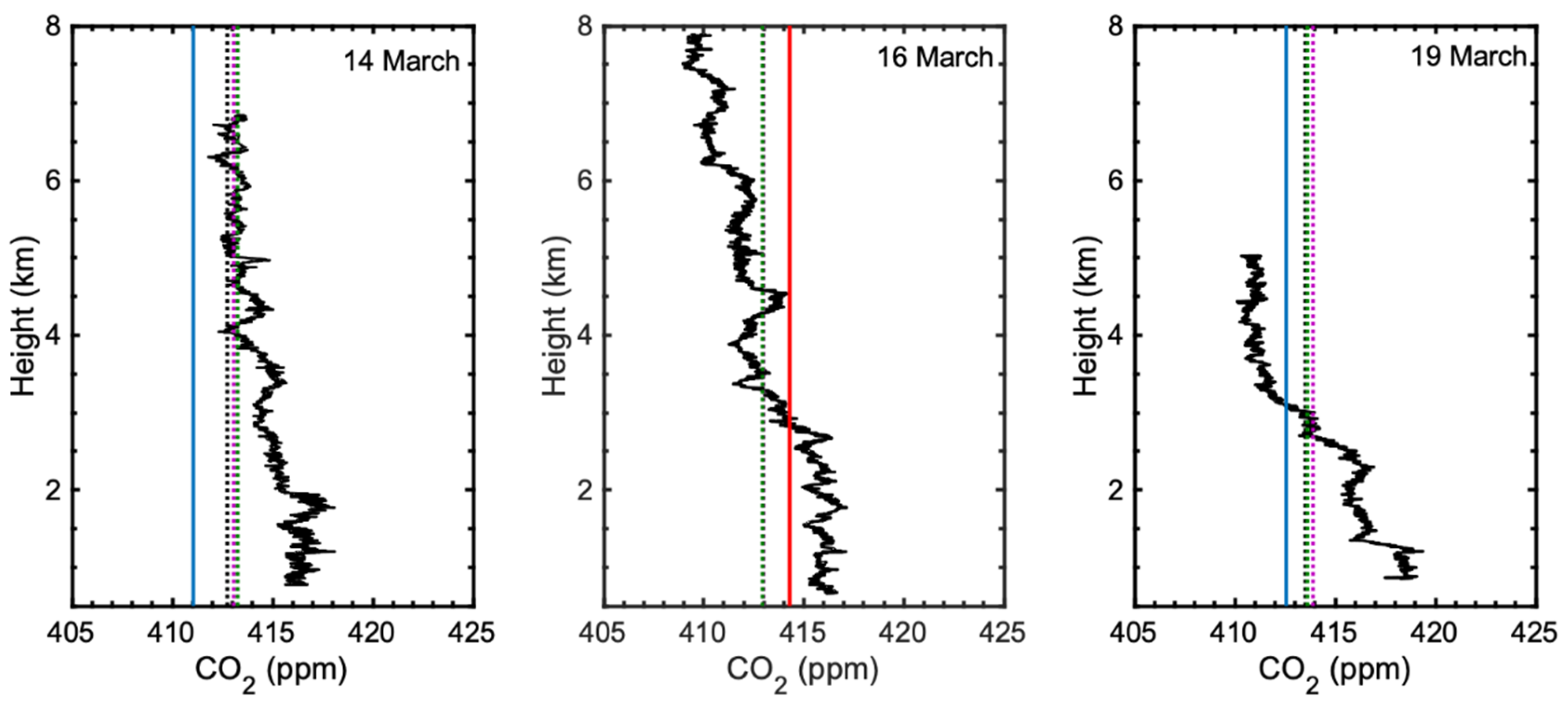
3.2. Comparison of Vertical Profiles

Figure 5 shows the in situ profiles measured by UGGA, GEOS-Chem, CarbonTracker, and satellite a priori for CO₂, along with corresponding column averaging kernels for CO₂ of GOSAT and OCO-2 on 14, 16, and 19 March 2019.

The averaging kernels of profile retrievals provide information about the contribution of the retrievals from a priori information and the measurements [64]. The CO₂ profiles from the models including GEOS-Chem and CarbonTracker were spatially interpolated to the location of the experimental site. The CO₂ concentration from in situ measurements is high near the surface and it generally decreases with increasing altitude. The high concentration of CO₂ near the surface is likely to be caused by strong anthropogenic emissions. In Northern China, the heating systems which are used in winter and spring consume a lot of fossil fuel energy, including oil, coal, and natural gas, and thus produce an excessive amount of CO₂ which is emitted into the atmosphere. As the temperature starts increasing from winter to spring, the microorganism activity also increases, and thus the enhanced decomposition process releases CO₂ from biological materials, which also contributes significantly to the increased atmospheric CO₂ [65]. In addition, the plants are in the dormant and recovery stage in winter and spring, so the weak photosynthesis and strong respiration in this season is also a potential reason for the increased CO₂ concentration [66,67]. The vertical profiles from all the products show the same varying trend, with some differences in their concentrations. The CO₂ concentration decreases gradually from surface to tropopause and exponentially in the stratosphere. The CO₂ concentration from GOSAT a priori is notably lower relative to other data products and this difference reaches nearly 3 ppm. GEOS-Chem and CarbonTracker show a similar vertical shape, but the CO₂ concentrations in the lower troposphere from these two models are larger than the aircraft measurements. LiPing et al. [68] compared the GOSAT observations with the measurements of GEOS-Chem and reported that GEOS-Chem results were 0.6 to 5.6 ppm higher than GOSAT over China. Mustafa et al. [3] compared OCO-2 and GOSAT observations with CarbonTracker CO₂ data over Asia and found that CarbonTracker showed a higher concentration of atmospheric CO₂ over China. The data driving the GEOS-Chem and CarbonTracker, the uncertainty of emissions caused by human activities, especially the fossil fuel burning, and differences in spatial resolutions might be among the main reasons behind the overestimations of model-simulated atmospheric CO₂ compared to in situ and satellite datasets. Previous studies have reported the poor performance of terrestrial flux from CT2015 against in situ observations obtained from eight sites of the Chinese Terrestrial Ecosystem Flux Observation and Research Network (ChinaFLUX) [69,70,71,72].

3.3. Uncertainty

The uncertainty in the aircraft-based XCO₂ is induced from three sources: (1) the profile above the maximum height, (2) the profile within the in situ measurements, and (3) the profile below the minimum height. The uncertainties induced by extrapolation of the aircraft profiles were analyzed separately for GOSAT and OCO-2. The missing profiles of the aircraft were extended by the three methods described above. For Method 1, no uncertainties were induced in the missing profiles because, in this method, the extrapolation was performed using the satellite a priori measurements, and the CO₂ concentrations of the missing parts were the same as those of the satellites. In Method 2 and Method 3, the unknown parts of the aircraft profile were extrapolated using GEOS-Chem and CarbonTacker CO₂ profiles, respectively. The stratospheric uncertainty is an important component and was calculated by shifting the stratospheric profile a priori up by 1 km and adding a shift of 1 ppm to the stratospheric a priori profile, based on the method discussed in a previous study [11]. More details about the uncertainty induced by extrapolation methods are given in

Table 5. The estimation of uncertainty for GOSAT induced by extrapolation Method 2 (GEOS-Chem CO₂ profiles) and Method 3 (CarbonTracker profiles).

Extrapolation	Date	Upper-Limit Errors (ppm)	Lower-Limit Errors (ppm)
Method 2	14 March 2019	0.63	0.092
	19 March 2019	0.79	0.21
Method 3	14 March 2019	0.67	0.069
	19 March 2019	0.91	0.13

and

Table 6. The estimation of uncertainty for OCO-2 induced by extrapolation Method 2 (GEOS-Chem CO₂ profiles) and Method 3 (CarbonTracker profiles).

Extrapolation	Date	Upper-Limit Errors (ppm)	Lower-Limit Errors (ppm)
Method 2	16 March 2019	0.39	0.072
Method 3	16 March 2019	0.39	0.070

. The uncertainties induced from the surface to the lower limit of the flight, and from the upper limit of flight to the stratosphere, are referred to as lower-limit errors and upper-limit errors, respectively. The extrapolation of missing profiles using GEOS-Chem and CarbonTracker shows no significant difference. This might be due to some similar inputs of the two models. Moreover, the uncertainty is relatively larger on 19 March and this might be due to the low vertical coverage (5000 m) of the flight because the extrapolation method recommended an altitude range of 6500–9500 m for accurate results [57].

4. Summary and Conclusions

China contributes significantly to the overall growth in global CO₂ emissions. Under the UNFCCC 2015 Paris Climate Agreement, China has pledged to reduce its CO₂ emissions per unit GDP by 60–65% relative to 2005 levels, and to peak carbon emissions overall, by 2030. However, the disagreement and uncertainties in the available data sources make it difficult for China to track progress toward these goals and evaluate the efficacy of control measures. In this study, the measurements of atmospheric vertical profiles of CO₂ were carried out using an aircraft over Qinhuangdao, China on 14, 16, and 19 March 2019 to validate the GOSAT and the OCO-2 CO₂ retrievals. The vertical distribution of CO₂ showed a decrease in the progression of altitude. Vertical profiles of GOSAT, OCO-2, GEOS-Chem, and Carbon-Tracker showed good agreement with the aircraft CO₂ measurements with the same varying trend; however, some differences were observed in their CO₂ concentrations. GOSAT observations showed a lower CO₂ concentration, while OCO-2, GEOS-Chem, and CarbonTracker showed higher CO₂ concentrations compared to in situ measurements. The data driving the GEOS-Chem and CarbonTracker, the uncertainty of emissions, and differences in spatial resolutions might be among the main reasons behind the higher concentration of atmospheric CO₂ found by the two models compared to in situ and satellite datasets. Moreover, XCO₂ retrieved from GOSAT and OCO-2 was compared with the column-averaged dry-air mole fraction of CO₂ calculated from the aircraft measurements. The results showed that GOSAT XCO₂ was underestimated by an amount of 1.70 ppm (0.41%), and OCO-2 measurements were overestimated by an amount of 1.33 ppm (0.39%). Results from this study and previous studies have shown larger uncertainties in satellite datasets over various regions of China. This is why several aircraft campaigns have been scheduled to be carried out in the near future with improved technologies including Integrated Path Differential Absorption (IPDA) Light Detection and Ranging (LIDAR) to monitor the atmospheric CO₂ over different regions of China.

References

1. Petit, J.R.; Raynaud, D. Forty years of ice-core records of CO2. Nature 2020, 579, 505–506. [Google Scholar] [CrossRef] [PubMed] [Green Version]
2. Dlugokencky Ed, T.P. Trends in Atmospheric Carbon Dioxide. Available online: ftp://aftp.cmdl.noaa.gov/products/trends/co2/co2_mm_gl.txt (accessed on 3 May 2020).
3. Mustafa, F.; Bu, L.; Wang, Q.; Ali, M.A.; Bilal, M.; Shahzaman, M.; Qiu, Z. Multi-year comparison of CO2 concentration from NOAA carbon tracker reanalysis model with data from GOSAT and OCO-2 over Asia. Remote Sens. 2020, 12, 2498. [Google Scholar] [CrossRef]
4. Jarraud, M.; Steiner, A. Climate Change 2014 Synthesis Report; IPCC: Geneva, Switzerland, 2012; Volume 9781107025, ISBN 9781139177245. [Google Scholar]
5. Sun, X.; Duan, M.; Gao, Y.; Han, R.; Ji, D.; Zhang, W.; Chen, N.; Xia, X.; Liu, H.; Huo, Y. In situ measurement of CO2 and CH4 from aircraft over northeast China and comparison with OCO-2 data. Atmos. Meas. Tech. 2020, 13, 3595–3607. [Google Scholar] [CrossRef]
6. Araki, M.; Morino, I.; MacHida, T.; Sawa, Y.; Matsueda, H.; Ohyama, H.; Yokota, T.; Uchino, O. CO2 column-averaged volume mixing ratio derived over Tsukuba from measurements by commercial airlines. Atmos. Chem. Phys. 2010, 10, 7659–7667. [Google Scholar] [CrossRef] [Green Version]
7. Zhang, D.; Tang, J.; Shi, G.; Nakazawa, T.; Aoki, S.; Sugawara, S.; Wen, M.; Morimoto, S.; Patra, P.K.; Hayasaka, T.; et al. Temporal and spatial variations of the atmospheric CO2 concentration in China. Geophys. Res. Lett. 2008, 35, 1–5. [Google Scholar] [CrossRef]
8. Schultz, M.G.; Akimoto, H.; Bottenheim, J.; Buchmann, B.; Galbally, I.E.; Gilge, S.; Helmig, D.; Koide, H.; Lewis, A.C.; Novelli, P.C.; et al. The global atmosphere watch reactive gases measurement network. Elementa 2015, 3, 000067. [Google Scholar] [CrossRef] [Green Version]
9. Yuan, Y.; Sussmann, R.; Rettinger, M.; Ries, L.; Petermeier, H.; Menzel, A. Comparison of continuous in-situ CO2 measurements with co-located column-averaged XCO2 TCCON/satellite observations and carbontracker model over the Zugspitze region. Remote Sens. 2019, 11, 2981. [Google Scholar] [CrossRef] [Green Version]
10. Toon, G.; Blavier, J.-F.; Washenfelder, R.; Wunch, D.; Keppel-Aleks, G.; Wennberg, P.; Connor, B.; Sherlock, V.; Griffith, D.; Deutscher, N.; et al. Total Column Carbon Observing Network (TCCON). In Proceedings of the Advances in Imaging, Vancouver, BC, Canada, 26–30 April 2009; Optical Society of America: Vancouver, BC, Canada, 2009; p. JMA3. [Google Scholar]
11. Wunch, D.; Toon, G.C.; Wennberg, P.O.; Wofsy, S.C.; Stephens, B.B.; Fischer, M.L.; Uchino, O.; Abshire, J.B.; Bernath, P.; Biraud, S.C.; et al. Calibration of the total carbon column observing network using aircraft profile data. Atmos. Meas. Tech. 2010, 3, 1351–1362. [Google Scholar] [CrossRef] [Green Version]
12. Wunch, D.; Wennberg, P.O.; Toon, G.C.; Connor, B.J.; Fisher, B.; Osterman, G.B.; Frankenberg, C.; Mandrake, L.; O’Dell, C.; Ahonen, P.; et al. A method for evaluating bias in global measurements of CO2 total columns from space. Atmos. Chem. Phys. 2011, 11, 12317–12337. [Google Scholar] [CrossRef] [Green Version]
13. Kulawik, S.; Wunch, D.; Dell, C.O.; Frankenberg, C.; Reuter, M.; Oda, T.; Chevallier, F.; Sherlock, V.; Buchwitz, M.; Osterman, G.; et al. Consistent evaluation of ACOS-GOSAT, BESD-SCIAMACHY, CarbonTracker, and MACC through comparisons to TCCON. Atmos. Meas. Tech. 2016, 9, 683–709. [Google Scholar] [CrossRef] [Green Version]
14. Hungershoefer, K.; Peylin, P.; Chevallier, F.; Rayner, P.; Klonecki, A.; Houweling, S.; Marshall, J. Evaluation of various observing systems for the global monitoring of CO2 surface fluxes. Atmos. Chem. Phys. 2010, 10, 10503–10520. [Google Scholar] [CrossRef] [Green Version]
15. Wang, H.; Jiang, F.; Wang, J.; Ju, W.; Chen, J.M. Differences of the inverted terrestrial ecosystem carbon flux between using GOSAT and OCO-2 XCO2retrievals. Atmos. Chem. Phys. Discuss. 2018, 19, 1–32. [Google Scholar] [CrossRef]
16. Taylor, T.E.; Eldering, A.; Merrelli, A.; Kiel, M.; Somkuti, P.; Cheng, C.; Rosenberg, R.; Fisher, B.; Crisp, D.; Basilio, R.; et al. OCO-3 early mission operations and initial (vEarly) XCO2 and SIF retrievals. Remote Sens. Environ. 2020, 251, 112032. [Google Scholar] [CrossRef]
17. Matsunaga, T.; Morino, I.; Yoshida, Y.; Saito, M.; Noda, H.; Ohyama, H.; Niwa, Y.; Yashiro, H.; Kamei, A.; Kawazoe, F.; et al. Early Results of GOSAT-2 Level 2 Products. In Proceedings of the AGU Fall Meeting Abstracts, San Francisco, CA, USA, 9–13 December 2019; Volume 2019, p. A52H-02. [Google Scholar]
18. Yang, D.; Liu, Y.; Cai, Z.; Chen, X.; Yao, L.; Lu, D. First Global Carbon Dioxide Maps Produced from TanSat Measurements. Adv. Atmos. Sci. 2018, 35, 621–623. [Google Scholar] [CrossRef]
19. Liu, Y.; Wang, J.; Yao, L.; Chen, X.; Cai, Z.; Yang, D.; Yin, Z.; Gu, S.; Tian, L.; Lu, N.; et al. The TanSat mission: Preliminary global observations. Sci. Bull. 2018, 63, 1200–1207. [Google Scholar] [CrossRef] [Green Version]
20. Crisp, D.; Miller, C.E.; DeCola, P.L. NASA Orbiting Carbon Observatory: Measuring the column averaged carbon dioxide mole fraction from space. J. Appl. Remote Sens. 2008, 2, 023508. [Google Scholar] [CrossRef]
21. Crisp, D. Measuring atmospheric carbon dioxide from space with the Orbiting Carbon Observatory-2 (OCO-2). In Proceedings of the Proc. SPIE, San Diego, CA, USA, 8 September 2015; Volume 9607. [Google Scholar]
22. Yokota, T.; Yoshida, Y.; Eguchi, N.; Ota, Y.; Tanaka, T.; Watanabe, H.; Maksyutov, S. Global Concentrations of CO2 and CH4 Retrieved from GOSAT: First Preliminary Results. SOLA 2009, 5, 160–163. [Google Scholar] [CrossRef] [Green Version]
23. Kiel, M.; O’Dell, C.W.; Fisher, B.; Eldering, A.; Nassar, R.; MacDonald, C.G.; Wennberg, P.O. How bias correction goes wrong: Measurement of XCO2 affected by erroneous surface pressure estimates. Atmos. Meas. Tech. 2019, 12, 2241–2259. [Google Scholar] [CrossRef] [Green Version]
24. Oshchepkov, S.; Bril, A.; Yokota, T.; Morino, I.; Yoshida, Y.; Matsunaga, T.; Belikov, D.; Wunch, D.; Wennberg, P.; Toon, G.; et al. Effects of atmospheric light scattering on spectroscopic observations of greenhouse gases from space: Validation of PPDF-based CO2 retrievals from GOSAT. J. Geophys. Res. Atmos. 2012, 117. [Google Scholar] [CrossRef] [Green Version]
25. Winderlich, J.; Chen, H.; Gerbig, C.; Seifert, T.; Kolle, O.; Lavrič, J.V.; Kaiser, C.; Höfer, A.; Heimann, M. Continuous low-maintenance CO2/CH4/H2O measurements at the Zotino Tall Tower Observatory (ZOTTO) in Central Siberia. Atmos. Meas. Tech. 2010, 3, 1113–1128. [Google Scholar] [CrossRef] [Green Version]
26. Inoue, M.; Morino, I.; Uchino, O.; Miyamoto, Y.; Yoshida, Y.; Yokota, T.; Machida, T.; Sawa, Y.; Matsueda, H.; Sweeney, C.; et al. Validation of XCO2 derived from SWIR spectra of GOSAT TANSO-FTS with aircraft measurement data. Atmos. Chem. Phys. 2013, 13, 9771–9788. [Google Scholar] [CrossRef] [Green Version]
27. Hedelius, J.K.; Parker, H.; Wunch, D.; Roehl, C.M.; Viatte, C.; Newman, S.; Toon, G.C.; Podolske, J.R.; Hillyard, P.W.; Iraci, L.T.; et al. Intercomparability of XCO2 and XCH4 from the United States TCCON sites. Atmos. Meas. Tech. 2017, 10, 1481–1493. [Google Scholar] [CrossRef] [Green Version]
28. Mendonca, J.; Strong, K.; Wunch, D.; Toon, G.C.; Long, D.A.; Hodges, J.T.; Sironneau, V.T.; Franklin, J.E. Using a speed-dependent Voigt line shape to retrieve O 2 from Total Carbon Column Observing Network solar spectra to improve measurements of XCO 2. Atmos. Meas. Tech. 2019, 12, 35–50. [Google Scholar] [CrossRef] [PubMed] [Green Version]
29. Wunch, D.; Wennberg, P.O.; Osterman, G.; Fisher, B.; Naylor, B.; Roehl, M.C.; O’Dell, C.; Mandrake, L.; Viatte, C.; Kiel, M.; et al. Comparisons of the Orbiting Carbon Observatory-2 (OCO-2) XCO2 measurements with TCCON. Atmos. Meas. Tech. 2017, 10, 2209–2238. [Google Scholar] [CrossRef] [Green Version]
30. Inoue, M.; Morino, I.; Uchino, O.; Nakatsuru, T.; Yoshida, Y.; Yokota, T.; Wunch, D.; Wennberg, P.O.; Roehl, C.M.; Griffith, D.W.T.; et al. Bias corrections of GOSAT SWIR XCO2 and XCH4 with TCCON data and their evaluation using aircraft measurement data. Atmos. Meas. Tech. 2016, 9, 3491–3512. [Google Scholar] [CrossRef] [Green Version]
31. Machida, T.; Matsueda, H.; Sawa, Y.; Nakagawa, Y.; Hirotani, K.; Kondo, N.; Goto, K.; Nakazawa, T.; Ishikawa, K.; Ogawa, T. Worldwide measurements of atmospheric CO2 and other trace gas species using commercial airlines. J. Atmos. Ocean. Technol. 2008, 25, 1744–1754. [Google Scholar] [CrossRef]
32. Frankenberg, C.; Kulawik, S.S.; Wofsy, S.C.; Chevallier, F.; Daube, B.; Kort, E.A.; O’Dell, C.; Olsen, E.T.; Osterman, G. Using airborne HIAPER pole-to-pole observations (HIPPO) to evaluate model and remote sensing estimates of atmospheric carbon dioxide. Atmos. Chem. Phys. 2016, 16, 7867–7878. [Google Scholar] [CrossRef] [Green Version]
33. NOAA/ESRL NOAA/ESRL Carbon Cycle Greenhouse Gases Aircraft Program. Available online: https://www.esrl.noaa.gov/gmd/ccgg/aircraft/ (accessed on 28 December 2020).
34. Tadić, J.M.; Loewenstein, M.; Frankenberg, C.; Butz, A.; Roby, M.; Iraci, L.T.; Yates, E.L.; Gore, W.; Kuze, A. A comparison of in situ aircraft measurements of carbon dioxide and methane to GOSAT data measured over railroad valley playa, nevada, USA. IEEE Trans. Geosci. Remote Sens. 2014, 52, 7764–7774. [Google Scholar] [CrossRef]
35. Agency, J.R.C.; (JRC)/PBL N.E.A. European Commission. Emission Database for Global Atmospheric Research (EDGAR v4.3.2). Available online: http://edgar.jrc.ec.europe.eu (accessed on 9 February 2021).
36. Shan, Y.; Guan, D.; Zheng, H.; Ou, J.; Li, Y.; Meng, J.; Mi, Z.; Liu, Z.; Zhang, Q. China CO2 emission accounts 1997–2015. Sci. Data 1997, 5, 1–14. [Google Scholar] [CrossRef] [Green Version]
37. UNFCC. Paris Agreement; United Nations: Paris, France, 2015.
38. Guan, D.; Liu, Z.; Geng, Y.; Lindner, S.; Hubacek, K. The gigatonne gap in China’s carbon dioxide inventories. Nat. Clim. Chang. 2012, 2, 672–675. [Google Scholar] [CrossRef]
39. Zhao, Y.; Nielsen, C.P.; McElroy, M.B. China’s CO2 emissions estimated from the bottom up: Recent trends, spatial distributions, and quantification of uncertainties. Atmos. Environ. 2012, 59, 214–223. [Google Scholar] [CrossRef]
40. Wang, W.; Tian, Y.; Liu, C.; Sun, Y.; Liu, W.; Xie, P.; Liu, J.; Xu, J.; Morino, I.; Velazco, V.A.; et al. Investigating the performance of a greenhouse gas observatory in Hefei, China. Atmos. Meas. Tech. 2017, 10, 2627–2643. [Google Scholar] [CrossRef] [Green Version]
41. Qu, Y.; Zhang, C.; Wang, D.; Tian, P.; Bai, W.; Zhang, X.; Zhang, P.; Dai, H.; Wu, Q. Comparison of atmospheric CO2 observed by GOSAT and two ground stations in China. Int. J. Remote Sens. 2013, 34, 3938–3946. [Google Scholar] [CrossRef]
42. Paul, J.B.; Lapson, L.; Anderson, J.G. Ultrasensitive absorption spectroscopy with a high-finesse optical cavity and off-axis alignment. Appl. Opt. 2001, 40, 4904–4910. [Google Scholar] [CrossRef] [PubMed]
43. Baer, D.S.; Paul, J.B.; Gupta, M.; O’Keefe, A. Sensitive absorption measurements in the near-infrared region using off-axis integrated-cavity-output spectroscopy. Appl. Phys. B 2002, 75, 261–265. [Google Scholar] [CrossRef]
44. Kuze, A.; Suto, H.; Nakajima, M.; Hamazaki, T. Thermal and near infrared sensor for carbon observation Fourier-transform spectrometer on the Greenhouse Gases Observing Satellite for greenhouse gases monitoring. Appl. Opt. 2009, 48, 6716–6733. [Google Scholar] [CrossRef]
45. Imasu, R.; Saitoh, N.; Niwa, Y.; Suto, H.; Kuze, A.; Shiomi, K.; Nakajima, M. Radiometric calibration accuracy of GOSAT-TANSO-FTS (TIR) relating to CO2 retrieval error. In Proceedings of the Proc. SPIE, Noumea, New Caledonia, 11 December 2008; Volume 7149. [Google Scholar]
46. Deng, A.; Yu, T.; Cheng, T.; Gu, X.; Zheng, F.; Guo, H. Intercomparison of Carbon Dioxide Products Retrieved from GOSAT Short-Wavelength Infrared Spectra for Three Years (2010-2012). Atmosphere 2016, 7, 109. [Google Scholar] [CrossRef] [Green Version]
47. Suntharalingam, P.; Jacob, D.D.; Palmer, P.I.; Logan, J.A.; Yantosca, R.M.; Xiao, Y.; Evans, M.J.; Streets, D.G.; Vay, S.L.; Sachse, G.W. Improved quantificaion of Chinese carbon fluxes using CO2/CO correlations in Asian outflow. J. Geophys. Res. Atmos. 2004, 109, 1–13. [Google Scholar] [CrossRef]
48. Nassar, R.; Jones, D.B.A.; Suntharalingam, P.; Chen, J.M.; Andres, R.J.; Wecht, K.J.; Yantosca, R.M.; Kulawik, S.S.; Bowman, K.W.; Worden, J.R.; et al. Modeling global atmospheric CO2 with improved emission inventories and CO2 production from the oxidation of other carbon species. Geosci. Model Dev. 2010, 3, 689–716. [Google Scholar] [CrossRef] [Green Version]
49. Van Der Werf, G.R.; Randerson, J.T.; Giglio, L.; Collatz, G.J.; Mu, M.; Kasibhatla, P.S.; Morton, D.C.; Defries, R.S.; Jin, Y.; Van Leeuwen, T.T. Global fire emissions and the contribution of deforestation, savanna, forest, agricultural, and peat fires (1997–2009). Atmos. Chem. Phys. 2010, 10, 11707–11735. [Google Scholar] [CrossRef] [Green Version]
50. Andres, R.J.; Gregg, J.S.; Losey, L.; Marland, G.; Boden, T.A. Monthly, global emissions of carbon dioxide from fossil fuel consumption. Tellus Ser. B Chem. Phys. Meteorol. 2011, 63, 309–327. [Google Scholar] [CrossRef] [Green Version]
51. Olsen, S.C.; Randerson, J.T. Differences between surface and column atmospheric CO2 and implications for carbon cycle research. J. Geophys. Res. Atmos. 2004, 109, 1–11. [Google Scholar] [CrossRef] [Green Version]
52. Baker, D.F.; Law, R.M.; Gurney, K.R.; Rayner, P.; Peylin, P.; Denning, A.S.; Bousquet, P.; Bruhwiler, L.; Chen, Y.H.; Ciais, P.; et al. TransCom 3 inversion intercomparison: Impact of transport model errors on the interannual variability of regional CO2 fluxes, 1988–2003. Glob. Biogeochem. Cycles 2006, 20, 1988–2003. [Google Scholar] [CrossRef] [Green Version]
53. Takahashi, T.; Sutherland, S.C.; Wanninkhof, R.; Sweeney, C.; Feely, R.A.; Chipman, D.W.; Hales, B.; Friederich, G.; Chavez, F.; Sabine, C.; et al. Corrigendum to “Climatological mean and decadal change in surface ocean pCO2, and net sea-air CO2 flux over the global oceans” [Deep Sea Res. II 56 (2009) 554-577] (doi:10.1016/j.dsr2.2008.12.009). Deep Res. Part I Oceanogr. Res. Pap. 2009, 56, 2075–2076. [Google Scholar] [CrossRef]
54. Fu, Y.; Liao, H.; Tian, X.J.; Gao, H.; Cai, Z.N.; Han, R. Sensitivity of the simulated CO2 concentration to inter-annual variations of its sources and sinks over East Asia. Adv. Clim. Chang. Res. 2019, 10, 250–263. [Google Scholar] [CrossRef]
55. Jacobson, A.R.; Fletcher, S.E.M.; Gruber, N.; Sarmiento, J.L.; Gloor, M. A joint atmosphere-ocean inversion for surface fluxes of carbon dioxide: 1. Methods and global-scale fluxes. Glob. Biogeochem. Cycles 2007, 21. [Google Scholar] [CrossRef]
56. Jacobson, A.R.; Schuldt, K.N.; Miller, J.B.; Tans, P.; Andrews, A.; Mund, J.; Aalto, T.; Bakwin, P.; Bergamaschi, P.; Biraud, S.C.; et al. CarbonTracker Near Real-Time, CT-NRT.v2020-1; NOAA ESRL: Boulder, CO, USA, 2020.
57. Tadić, J.M.; Biraud, S.C. An approach to estimate atmospheric greenhouse gas total columns mole fraction from partial column sampling. Atmosphere 2018, 9, 247. [Google Scholar] [CrossRef] [Green Version]
58. Rodgers, C.D.; Connor, B.J. Intercomparison of remote sounding instruments. J. Geophys. Res. D Atmos. 2003, 108. [Google Scholar] [CrossRef] [Green Version]
59. Morino, I.; Uchino, O.; Inoue, M.; Yoshida, Y.; Yokota, T.; Wennberg, P.O.; Toon, G.C.; Wunch, D.; Roehl, C.M.; Notholt, J.; et al. Preliminary validation of column-averaged volume mixing ratios of carbon dioxide and methane retrieved from GOSAT short-wavelength infrared spectra. Atmos. Meas. Tech. 2011, 4, 1061–1076. [Google Scholar] [CrossRef] [Green Version]
60. Yoshida, Y.; Kikuchi, N.; Morino, I.; Uchino, O.; Oshchepkov, S.; Bril, A.; Saeki, T.; Schutgens, N.; Toon, G.C.; Wunch, D.; et al. Improvement of the retrieval algorithm for GOSAT SWIR XCO2and XCH4and their validation using TCCON data. Atmos. Meas. Tech. 2013, 6, 1533–1547. [Google Scholar] [CrossRef]
61. Liang, A.; Gong, W.; Han, G.; Xiang, C. Comparison of satellite-observed XCO2 from GOSAT, OCO-2, and ground-based TCCON. Remote Sens. 2017, 9, 1033. [Google Scholar] [CrossRef] [Green Version]
62. Oh, Y.S.; Kenea, S.T.; Goo, T.Y.; Chung, K.S.; Rhee, J.S.; Ou, M.L.; Byun, Y.H.; Wennberg, P.O.; Kiel, M.; Digangi, J.P.; et al. Characteristics of greenhouse gas concentrations derived from ground-based FTS spectra at Anmyeondo, South Korea. Atmos. Meas. Tech. 2018, 11, 2361–2374. [Google Scholar] [CrossRef] [Green Version]
63. Randel, W.J.; Wu, F.; Gaffen, D.J. Interannual variability of the tropical tropopause derived from radiosonde data and NCEP reanalyses. J. Geophys. Res. Atmos. 2000, 105, 15509–15523. [Google Scholar] [CrossRef]
64. Olsen, K.S.; Strong, K.; Walker, K.A.; Boone, C.D.; Raspollini, P.; Plieninger, J.; Bader, W.; Conway, S.; Grutter, M.; Hannigan, J.W.; et al. Comparison of the GOSAT TANSO-FTS TIR CH volume mixing ratio vertical profiles with those measured by ACE-FTS, ESA MIPAS, IMK-IAA MIPAS, and 16 NDACC stations. Atmos. Meas. Tech. 2017, 10, 3697–3718. [Google Scholar] [CrossRef] [Green Version]
65. Anthwal, A.; Joshi, V.; Joshi, S.; Sharma, A.; Kim, K.-H. Atmospheric Carbon Dioxide Levels in Garhwal Himalaya, India. J. Korean Earth Sci. Soc. 2009, 30, 588–597. [Google Scholar] [CrossRef] [Green Version]
66. Miao, R.; Lu, N.; Yao, L.; Zhu, Y.; Wang, J.; Sun, J. Multi-year comparison of carbon dioxide from satellite data with ground-based FTS measurements (2003–2011). Remote Sens. 2013, 5, 3431–3456. [Google Scholar] [CrossRef] [Green Version]
67. Zhou, T.; Yi, C.; Bakwin, P.S.; Zhu, L. Links between global CO2 variability and climate anomalies of biomes. Sci. China Ser. D Earth Sci. 2008, 51, 740–747. [Google Scholar] [CrossRef]
68. Lei, L.P.; Guan, X.H.; Zeng, Z.C.; Zhang, B.; Ru, F.; Bu, R. A comparison of atmospheric CO2 concentration GOSAT-based observations and model simulations. Sci. China Earth Sci. 2014, 57, 1393–1402. [Google Scholar] [CrossRef]
69. Yu, G.-R.; Wen, X.-F.; Sun, X.-M.; Tanner, B.D.; Lee, X.; Chen, J.-Y. Overview of ChinaFLUX and evaluation of its eddy covariance measurement. Agric. For. Meteorol. 2006, 137, 125–137. [Google Scholar] [CrossRef]
70. Yu, G.; Fu, Y.; Sun, X.; Wen, X.; Zhang, L. Recent progress and future directions of ChinaFLUX. Sci. China Ser. D Earth Sci. 2006, 49, 1–23. [Google Scholar] [CrossRef]
71. Yu, G.-R.; Zhang, L.-M.; Sun, X.-M.; Fu, Y.-L.; Wen, X.-F.; Wang, Q.-F.; Li, S.-G.; Ren, C.-Y.; Song, X.I.A.; Liu, Y.-F.; et al. Environmental controls over carbon exchange of three forest ecosystems in eastern China. Glob. Chang. Biol. 2008, 14, 2555–2571. [Google Scholar] [CrossRef]
72. Yu, G.-R.; Zhu, X.-J.; Fu, Y.-L.; He, H.-L.; Wang, Q.-F.; Wen, X.-F.; Li, X.-R.; Zhang, L.-M.; Zhang, L.; Su, W.; et al. Spatial patterns and climate drivers of carbon fluxes in terrestrial ecosystems of China. Glob. Chang. Biol. 2013, 19, 798–810. [Google Scholar] [CrossRef] [PubMed]
Figure 1. The schematic diagram of the off-axis Integrated Cavity Output Spectroscopy (ICOS) instrument.
Remotesensing 13 00899 g001
Figure 2. The experimental site for aircraft-based measurements of CO2 and the flight paths on (a) 14 March (b) 16 March, and (c) 19 March 2019 over Qinhuangdao, China. The yellow points show the satellite observations near the study area.
Remotesensing 13 00899 g002
Figure 3. The flight trajectory on 16 March 2019 over Qinhuangdao, China. The color bar represents the progression of time, where blue represents the starting time and red represents the ending time.
Remotesensing 13 00899 g003
Figure 4. In situ CO2 profiles measured by the UGGA and the column-averaged mole fraction CO2 derived using various extrapolation methods: from satellite a priori profiles (Method 1), from GEOS-Chem CO2 profiles (Method 2), and from the CarbonTracker CO2 profiles (Method 3), along with GOSAT and OCO-2 XCO2 measurements for 14, 16, and 19 March 2019.
Remotesensing 13 00899 g004
Figure 5. The CO2 profiles from Aircraft, GEOS-Chem, CarbonTracker, GOSAT, and OCO-2 along with their corresponding column averaging kernels (CAK) for 14, 16, and 19 March 2019 over Qinhuangdao, China. The red line shows the extrapolation of the aircraft measurements using satellite a priori data. The horizontal line represents the tropopause height which was calculated using the National Centers for Environmental Prediction (NCEP) reanalysis dataset [63].
Remotesensing 13 00899 g005