
Building Extraction and Number Statistics in WUI Areas Based on UNet Structure and Ensemble Learning


1
Aerospace Information Research Institute, Chinese Academy of Sciences, Beijing 100094, China
2
College of Resources and Environment (CRE), University of Chinese Academy of Sciences, Beijing 100049, China
*
Author to whom correspondence should be addressed.
Remote Sens. 2021, 13(6), 1172; https://doi.org/10.3390/rs13061172
Submission received: 18 February 2021
/
Revised: 14 March 2021
/
Accepted: 16 March 2021
/
Published: 19 March 2021
(This article belongs to the Special Issue AI Interpretation of Satellite, Aerial, Ground, and Underwater Image and Video Sequences)
Abstract
:Following the advancement and progression of urbanization, management problems of the wildland–urban interface (WUI) have become increasingly serious. WUI regional governance issues involve many factors including climate, humanities, etc., and have attracted attention and research from all walks of life. Building research plays a vital part in the WUI area. Building location is closely related with the planning and management of the WUI area, and the number of buildings is related to the rescue arrangement. There are two major methods to obtain this building information: one is to obtain them from relevant agencies, which is slow and lacks timeliness, while the other approach is to extract them from high-resolution remote sensing images, which is relatively inexpensive and offers improved timeliness. Inspired by the recent successful application of deep learning, in this paper, we propose a method for extracting building information from high-resolution remote sensing images based on deep learning, which is combined with ensemble learning to extract the building location. Further, we use the idea of image anomaly detection to estimate the number of buildings. After verification on two datasets, we obtain superior semantic segmentation results and achieve better building contour extraction and number estimation.
1. Introduction
The wildland–urban interface (WUI), a formal land classification specification, first appeared in the research budget of the US Forest Service in 1978. It is used for urban areas that need to be strengthened for fire protection [1]. Because the WUI is located at the boundary between the city and the wasteland, mountain fires caused by climate change or human factors are likely to affect the residential areas. Moreover, it is not only fire itself that threatens the city but also precipitation after fires, which may evolve into floods and debris flows, increasing the harm to residents and local infrastructures [2]. Therefore, the management of this kind of area cannot be simply considered the same as that for a wasteland. In recent years, with the acceleration of urbanization and the deepening of climate change, extreme weather events of forest fires have become more frequent and serious [3]. With the emergence of several global fires in recent years, researchers worldwide are very concerned about fires in WUI areas and their prevention.
In China, with the expansion of the urban area, the urban active population continues to shift to the suburbs and the forest areas. Many areas with WUI characteristics were objectively formed and have become increasingly large. Due to the lack of relevant management practices, some buildings located at the boundary between the city and the wasteland often suffered losses because of sudden forest fires. In the WUI area, the core issue of people’s concern is always the safety of property and life. Among many solutions, setting up related management measures for buildings is an effective method. In foreign countries, Manzello et al. conducted research on building specifications about building materials and structures under the threat of WUI fires [4]. Kowronski et al. propose to delineate a certain buffer zone around the building domain for fire protection [5]. As determined from the above studies, scholars have attempted many approaches to protect buildings from fire damage. However, there are still many deficiencies in the research on obtaining information about buildings from the WUI area.
Remote sensing methods provide information with a large sensing range and rapid acquisition speed. Using remote sensing image, we can quickly scan the WUI-related area to obtain the ground profile and identify fine features of ground objects, satisfying the objectives of global browsing demands to support all needs of disaster monitoring, rescue command and post-disaster governance based on detailed information. In recent years, researchers have used aerial photographs and general surveys of ground personnel to conduct building damage assessments, and they found that remote sensing methods can more easily and accurately obtain information regarding roof damage to buildings [6]. For decades, researchers have attempted different methods and combined different remote sensing data to extract building information. In 2014, Awrangjeb used LIDAR data combined with local DEM data to extract buildings and building roofs [7]. In 2018, Awrangjeb proposed an improved interpolation method to preserve the geometric features of buildings in order to better distinguish between buildings and vegetation in LIDAR [8]. Zhang et al. used UAV data to establish a process for extracting information about damaged buildings after an earthquake, and the approach can still operate on cloudy and rainy days, providing great helps for disaster relief [9]. Zhiqiang et al. used high-resolution remote sensing data, combined with object-oriented segmentation and semantic segmentation, and achieved good results in building change detection [10]. It is not difficult to determine from recent studies that the use of remote sensing methods to extract building information for WUI areas offers both macroscopic and comprehensive advantages. Using high-resolution remote sensing data to extract information for building clusters in WUI areas can effectively make a WUI regional building management strategy. However, in many studies, scholars mostly use handcrafted features to extract buildings, which is inefficient and not accurate enough.
In the past few years, deep learning algorithms have made breakthrough progress in the field of image processing, and the effects of remote sensing information extraction have also been greatly improved with the rapid development of artificial intelligence. There are increasingly more researchers attempting to extract information in combination with artificial intelligence algorithms. In 2016, Guo et al. used CNN and Adaboost ensemble learning methods to extract villages in remote sensing images based on Google images [11]. In 2017, Chen et al. used the RCNN network to improve the problem of detecting rectangular frames that could not be rotated, and they conducted a building extraction test on a public dataset [12]. In the same year, Bittner et al. introduced DSM data and used a fully convolutional network to extract buildings [13]. In 2018, Yang et al. used convolutional networks to extract buildings on several continents and mapped them into maps in the United States [14]. In the same year, Li Xiang et al. used the adversarial network method to obtain the optimal segmentation map of a building [15]. Xu et al. improved the structure of the UNet network and combined it with the guided filter to extract buildings, and they conducted experiments on two public datasets, achieving improved results [16]. In 2019, Li et al. comprehensively considered four kinds of neural network structures and extracted the developed urban areas [17]. In 2020, Wu et al. used a frameless building instance segmentation scheme to extract suburban buildings [18]. Lu Beiru et al. proposed a deep learning-related improvement plan for urban buildings [19].
As seen from the above studies, many methods for building research have achieved good results. However, the following two problems remain in the above research. One issue is that the dataset used mainly pertains to urban areas, and the relevant methods are not effective when applied to WUI areas. Regardless of whether the research endeavors for building extraction occur in Chinese or international industry, they are mostly concentrated according to the improvement of popular algorithms. The datasets employed are mostly from dense urban building areas or international public datasets. However, WUI area buildings are different from urban buildings: they have a high density of aggregation, different shapes, and irregular distributions. At the same time, buildings in mountainous areas are easily blocked by trees, which brings great difficulties to building information extraction. Another consideration is that research on building information extraction algorithms is not suitable for practical applications. There are also many omissions and misclassifications in densely built areas. It often occurs that several buildings are detected as one building, so it is not sufficiently accurate to directly calculate the number of buildings using the results of instance segmentation or target detection.
Therefore, in this paper, we propose a method for extraction of building information and calculating its number based on deep learning. Relevant research was conducted in the Yaji Mountain National Forest Scenic Area in Pinggu District, Beijing. We chose the semantic segmentation network with the highest overall extraction accuracy as the basic information extraction network. We chose the Unet network framework among many semantic segmentation networks. Considering the complex situations of buildings in the WUI area, we adjusted many parameters to improve the model and used ensemble learning to integrate models, thus improving the accuracy of building extraction in WUI. According to our semantic segmentation results, we evaluated the effects of building segmentation and further estimated the number of buildings in the research area. To ensure the applicability of the method, we also conducted experiments on the public WHU building dataset produced by Wuhan University. The main contributions of our work are summarized as follows:
- A technical method for constructing a dataset in the research area based on high-resolution remote sensing data is proposed. We use an extraction algorithm that only requires a small number of samples to extract some buildings, reducing the labor and time costs required for deep learning sample production.
- We also propose a method of organically combining deep learning and integrated learning. After researching the WUI region, we have identified data augmentation, loss function adjustment, and other ways to optimize the model. We trained the network with different parameters to obtain deep learning models with large differences and then selected from these models. Finally, all selected models were integrated to predict the final semantic segmentation results.
- To further obtain the number of buildings in the area, in this paper, we use the generative adversarial network to identify and reconstruct the image of a single building based on the results of the semantic segmentation of the building. Then, we separate single buildings and non-single buildings from the semantic segmentation results and finally estimate the number of buildings in the extracted results by using the building area.
The full text is organized as follows. Section 2 introduces building information extraction methods based on comprehensive ensemble learning and UNet semantic segmentation and application methods based on adversarial neural networks. Section 3 introduces the remote sensing images used in the experiment, the experimental area, the datasets that we used and accuracy evaluation methods used in the experiment. Section 4 introduces the experimental results and analyzes the details. Section 5 summarizes the article and looks forward to future directions of continuous efforts to improve and perfect this work.
2. Methods
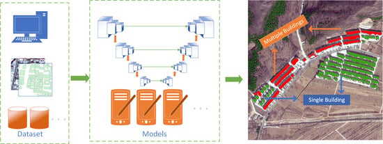
The overall structure of our complete work is shown in Figure 1, which is mainly composed of three parts. Figure 1a is to quickly construct a sample set through remote sensing images, Figure 1b is to use the constructed sample set to train to obtain a better model, and Figure 1c is to use our prediction results for further application. It is described in detail as follows: The first part includes the rapid construction of sample sets in the WUI area and some processes of remote sensing image preprocessing. The sample set construction is shown in Figure 1a, where the overall construction process includes three steps. First, we preprocess remote sensing images to obtain high-resolution image results with geographic coordinates; second, we use machine learning algorithms to distinguish some of the images that are easy to distinguish; finally, some previous targets are checked and manually corrected, and the remaining unidentified vector parts are added. Figure 1b introduces our building semantic information extraction process. In this step, we modify the parameters of the basic UNet network structure so that the network trains to obtain different models, and we select the model results that we need through correlation-based feature selection (CFS) adaptive search. Finally, the selected model prediction results are integrated to obtain our final semantic segmentation results. Figure 1c introduces our idea for distinguishing the number of buildings from the results of semantic segmentation. It mainly consists of two parts. The first part uses the idea of the generative adversarial network (GAN) to make a fuzzy judgment regarding the number of buildings [20], which can distinguish whether the image includes a single building or multiple buildings. The second part is a relatively accurate estimation of the number of buildings in the area, which utilizes the result of the fuzzy judgment in the previous step. We divide the area of the results of multiple buildings by the regional average of the results of a single building to calculate the final number of buildings.
2.1. Construction of a Sample Set
To reduce labor costs, we propose a scheme to simplify the construction of building samples. The main idea is to extract buildings that can be recognized by the general machine learning algorithm, these buildings will be converted into a vector. The specific process results are shown in Figure 2. We use multiple steps including algorithmic rough extraction, smoothing denoising, corrosion expansion, and edge search vectorization to obtain our pre-extraction results. In our experiments, we used the maximum likelihood classification method to perform preliminary building target extraction and then used the 3 × 3 morphological operator to perform multiple corrosion expansion to smooth the edge of the building. Finally, the obtained raster extraction results are converted to ArcGIS supported by the Python GDAL library shape vector format:
The quantity of data in a single remote sensing image is too large to be read at one time for training because of limited computer memory. For example, the image size used in our experiment is 10,673 × 20,220, but the image size usually used in deep learning training is approximately 500 × 500 and generally does not exceed 1500 × 1500. Therefore, the image needs to be segmented before deep learning model training. In addition, controlling the ratio between positive samples and negative samples to prevent most training samples from having no target will make our model difficult to fit. Usually, we also need to ensure that our target is within the cutting range when performing sample segmentation. Figure 3 shows one of the slice results that we obtained.
After completing the labeling and data cutting of actual data, we selected some data transformation methods to enhance our dataset for the WUI region. Data augmentation can increase the diversity of data and make the trained models more stable; it is a common data preprocessing method in the field of deep learning. The existing data augmentation effect is better in the form of random combination using several conventional data transformation methods. The data transformation methods selected in this article are color adjustment, data mirroring, image scale adjustment, rotation, and cropping. In this study, we control whether the data augmentation is performed and the specific augmentation amplitude by generating a random number. The specific operations are the following: (1) Convert the original image to HSV space and generate a random number not less than a given value. This random number is subtracted or added to the three bands of H, S, and V, and then, the image is converted to RGB. (2) For random mirroring, generate a random number between 0–1; if it is greater than the given value, mirror the original image and the corresponding label horizontally. (3) For random rotation, also randomly generate a random value that is not less than a given value; rotate the image and label clockwise according to the random value. The given value that we use here is 60 degrees. (4) Randomly adjust the scale, randomly generate a scale factor not less than 1 and not greater than the given scale factor, and enlarge the image and the corresponding label. The scale factor given in our experiment is 1.5. (5) Given a crop size, randomly crop an area in the rotated image. The crop size given in this article is 500. The specific content is shown in Figure 4.
2.2. UNet Network Structure
In recent years, deep learning has become the most advanced tool for pixel classification in remote sensing and other fields. Fully convolutional networks are used as an effective tool for semantic labeling of high-resolution remote sensing data [16]. In 2015, Ronneberger et al. proposed the UNet semantic segmentation network for medical image segmentation, especially for cell segmentation [21]. The UNet network structure follows the encoding–decoding structure of its predecessors, and on this basis, each upsampling is fused with the same scale as the number of channels corresponding to the feature extraction part. This design greatly relieves the space constraint caused by downsampling and the loss of information improves the accuracy of semantic segmentation. The extraction of buildings from remote sensing images has certain similarities with the extraction of cells from medical images. In recent years, it has also been determined that the use of the UNet network to extract buildings from remote sensing images has achieved better results [16,22,23]. In this article, the main body still uses the Unet network structure, and the overall network structure is as shown in Figure 5.
2.3. Ensemble Learning
Ensemble learning completes the learning task by combining multiple models. The general strategy of ensemble learning is to generate a group of “individual learners” and then to use a certain strategy to combine them. The model selection of ensemble learning follows the principle of “good but different”; that is, it will be better to use several models with higher accuracy and greater model differences for joint prediction. During training, the convolutional neural network itself saves multiple models according to the different effects on the validation set. There are natural differences between the models, which meets the application conditions of ensemble learning to a certain extent. Second, there are many parameters and hyperparameters of convolutional neural networks. In the process of adjusting the training parameters, there is often a model effect without breakthrough, but the prediction results are very different. These models naturally also conform to the application of ensemble learning. Therefore, when the accuracy of the model is difficult to improve, considering that the ensemble learning method has become another effective approach. The process is roughly shown in Figure 6. Through different parameter adjustments on the basic network, different prediction results are generated. The results are then integrated according to the voting method to produce the final result.
Choosing a suitable model is the most critical step in ensemble learning. The key to model selection is the evaluation of a single model and a combination of different models. The accuracy evaluation method of the model is shown in Section 3.2. Through Formulas (5)–(7), we select a series of initial models with improved accuracy. Then, we use Formula (1) to calculate the correlation coefficient r of the model, and the correlation number r is used to measure the correlation between the two models. The weaker the model correlation is, the closer the value is to 0. However, there is a natural contradiction between diversity and accuracy. Generally, the model trained by the network has higher accuracy, so the correlation coefficient value r is generally close to 1. The meanings of the parameters in Formula (1) are shown in Table 1, a represents the number of positions where the two models have positive result in the image, b and c represent that the two prediction results are 1 positive and 1 negative, and d represents that the two prediction results are both negative.
We then obtain the results of multiple models as displayed in the table, and the difference matrix of the model is shown in Table 2. To select the best model combination, we use CFS (correlation based feature selection). The core of the feature search is to use a heuristic search method to search the model with the largest difference [24]. After obtaining the correlation matrix of all models, we evaluate the value of each model or model combination by calculating the heuristic equation metric, and then, we can obtain our optimal model by forward search. The calculation method for the metric is shown in Formula (2), where k represents the k-th model, represents the correlation coefficient between the predicted results of the model and the real situation, and represents the correlation coefficient between the models.
Finally, these selected models are integrated by using the classical voting method in ensemble learning. For our problem, the value of a pixel in the prediction result can be regarded as the probability of buildings in the image. Therefore, we sum the probability values of the outputs of these models and divide them by the number of models to obtain a probability average of the overall prediction results. If the probability is greater than 0.5, it is considered a building.
2.4. Single Building Detection and Number Statistics
Traditional semantic segmentation can only be done in the previous step, but such results are limited in the practical applications of buildings. After obtaining the semantic segmentation results of the buildings, we only acquire the approximate distribution of the buildings, whereas most practical applications are for a specific building. Therefore, we combine the nearby pixels and convert our semantic segmentation results into instance results to achieve our object-level applications. In the experiment, we used the Unicom domain function (named cv::connectedComponents) provided by OpenCV to aggregate pixels to extract different objects. The specific effect is shown in Figure 7, where Figure 7a is the original image, Figure 7b is the semantic segmentation result, and Figure 7c is the result of the semantic segmentation instantiated by the OpenCV algorithm.
In our object-level results, there are not only some results with one building but also some results with multiple buildings. Because of the dense distribution of buildings in the WUI area, in our semantic segmentation results, the phenomenon that the predicted pixels are classified as a building is particularly common in our study area. We distinguish between single buildings and non-single buildings by referring to the idea of abnormal image detection [20]. We use the images of individual buildings in our original training data to train the network and then use the trained network model to predict the extraction results of our semantic segmentation. The result of this anomaly detection adversarial network is called GanalyNet in [20], which uses the GAN to reconstruct images. The fake image “Fake Image” is reconstructed through the encoding–decoding structure, and then, an encoder is used to encode the real image and the generated image into a 100 × 1 vector, and the difference between the vectors (real image and fake image) is compared to determine whether the image is abnormal. The specific structure is shown in Figure 8, the green vector is the encoding vector before image reconstruction, and the red is the encoding vector after reconstruction. The reconstruction loss of the image can be calculated by the formula in the upper right corner. Two curves in the lower right corner shows the difference in reconstruction loss of different image types.
The essence of our building discrimination method is anomalous image detection. The network training only uses images containing a single building. Therefore, when inputting an image containing a single building to determine the reconstruction loss, the reconstruction error is small, but when the input containing images of multiple buildings is used for judgment, the reconstruction error is large. Therefore, by comparing the generated vector difference, whether the input image is a picture containing a single building can be judged. As shown in Figure 8, the entire confrontation network is composed of a generator and a discriminator. The discriminator is a simple two-class network, and the generator adopts an encoding–decoding–re-encoding structure. Figure 8 presents the specific details to the reader. There are two key points in the whole structure. One key point is the downsampling during structure encoding. To fully preserve the position information and texture details, the downsampling mainly uses the convolution function with step size. The second key point is the design of the loss function. Here, there are two main loss functions related to the generator part: encoding vector loss and reconstruction loss. Among them, reconstruction loss is the most important and controls the fitting of the entire network. Generally, its loss accounts for the entire network loss of more than 90 percent. The vector loss is our criterion for anomaly discrimination. The larger the value is, the greater the possibility of anomalies. In our application, the greater the value is, the greater the probability that the image contains more than one building.
To produce the final statistics regarding the number of buildings in the WUI area, we estimate the number of buildings in different areas using the building results that we have extracted. The specific method is to obtain the average value of the area of a single building in different regions by a statistical method and then to divide the area of the buildings in an image with multiple buildings that we judged by this average value. In this way, the number of buildings included in an image with more than one building can be obtained, and the number of buildings that we estimate is ultimately obtained.
3. Dataset and Evaluation Metrics
3.1. Dataset
Because this article mainly studies the emergency events in the WUI area, to ensure that the monitoring area can obtain the data as soon as possible, we used the domestic remote sensing data SuperView-1 for the experiment, for which the spatial resolution of the panchromatic band of the data is 0.5 m, and the spatial resolution of the multispectral band is 1 m, including R, G, B, and NIR bands. This paper used the fusion result of 0.5 m resolution to carry out follow-up experiments. The main area of the experiment was Yaji Mountain which is located in Liujiadian, Pinggu District, Beijing, and is a famous Taoist holy land in North China. On 30 March 2019, there was a forest fire in this area, so the study of this event has important significance for similar WUI areas in the country. The specific situation of the field is shown in Figure 9. There are two scenes of SuperView-1 data. Figure 9a shows the data of one scene in summer. The red frame in the picture shows our test area. Figure 9a shows the data of a winter scene, which is geographically located to the east of Figure 9b. Among them, the summer data test area includes a total of 1558 buildings, and the training area includes 2114 buildings. The winter data are actually used as a supplement to the training data. The winter data include a total of 16,154 buildings. The data in the training area and the test area were partitioned into the size of 512 × 512 to produce our final sample set, which is called the YJS (which is named “Yaji Shan” in Chinese Pinyin) dataset in the following experiments.
To enhance the credibility of our plan, in addition to the research area dataset, we conducted experiments on the public dataset WHU, which is an open source dataset. The original images are from the New Zealand land information service network, and the image coverage is located in New Christchurch, New Zealand (http://study.rsgis.whu.edu.cn/pages/download/building_dataset.html; WHU building Dataset, access on 18 February 2021). By sampling most of the aerial images (including 187,000 buildings) to a ground resolution of 0.3 m, the samples to be used are divided into three parts: training set (130,500 buildings), verification set (14,500 buildings), and test set (42,000 buildings). The final dataset results include 4736 images of the training set, 2016 images of the test set, and 1036 images of the verification set; Figure 10 shows the slicing results of one image.
3.2. Evaluation
When using remote sensing data to analyze ground features, our targets are generally relatively sparse within the entire remote sensing image. With traditional overall accuracy (OA), our true target situation will be covered by substantial background, which cannot reflect the actual situation of our targets very well. Therefore, this paper uses the F1 score to evaluate our building extraction results. The F1 score is the reconciled average value of the recall rate and accuracy rate according to the specific formulas as shown in Formulas (5)–(7):
where TP denotes true positive, FP denotes false positive, and FN denotes false negative. These indicators are calculated using each tiled pixel-based confusion matrix or cumulative confusion matrix and are explained as follows. If the real situation in a region is a building and the prediction is also a building, then the pixels are marked as TP. If the real pixel is a building but the prediction is not a building, then the pixels are marked as FN. If the real pixel is not a building but is predicted to be a building, then the pixel is of type FP.
4. Results
In this article, we use the above methods to conduct experiments. To predict the study area through the network, we can acquire the results of two parts. The first part is the semantic segmentation. By adjusting the model structure and training parameters, we obtain the prediction models under different conditions and then use the idea of ensemble learning to obtain the final result of our semantic segmentation. The second part is the reprocessing result of the semantic segmentation result, including the processing of the connectivity result, the identification of the number of buildings in the image, and the estimation of the number of buildings. The overall extraction results are shown in Figure 11. We show our testing on the YJS dataset and WHU dataset. Figure 11a–e display the testing process of the WHU dataset, and Figure 11f–j present the results on the YJS dataset.
Subsequently, this article introduces the basic situation of each part of our experiment. In Section 4.1, this article introduces the evaluation of several basic network frameworks and the reason for finally choosing the Unet framework as the basic structure. In Section 4.2, we introduce our application of integrated learning to improve semantic segmentation accuracy. In Section 4.3, this article introduces the entire experimental process of further extracting the number of buildings based on the semantic segmentation results. Finally, in Section 4.4, we briefly introduce the experimental situation using our building number estimation. In addition, Some more detailed parameter settings can be seen in Table 3.
4.1. Basic Network Structure
In the evaluation of basic network structure, we evaluated the classification effects of DeepLab V3, FCN, and UNET on the WHU dataset and YJS dataset. By optimizing the same parameters for different network structures, we have obtained the optimal extraction structure for each frame structure in the building extraction task. After comparison, first, the UNet network structure has achieved the best prediction results on both datasets. Second, the effects of the network model on different datasets are also different. On the publicly available WHU training dataset, the results achieved by several models are relatively small, while the difference is large for the YJS dataset that we produced. The specific results are shown in Table 4.
In addition to the choice of the basic network framework, we used more solutions to optimize the extraction results. After conducting continuous model adjustment research, we optimized the model results in terms of data augmentation, loss function, and sample adjustment of the dataset. Experiments have proven that the adjustment of these parameters brings better extraction effects to the model during building extraction tasks for WUI areas. The specific experimental accuracy is shown in Table 5. The data augmentation mainly includes geometric augmentation and optical transformation. The results are shown in M1–M3 of the table. The loss function transformation is mainly performed to adjust the proportions of positive and negative samples in the loss function. The results are shown in M4–M6 of the table. The adjustment of the samples in the final sample set is mainly performed to adjust the proportion of a single sample. The results are shown in M7–M9.
4.2. Ensemble Learning
After the model is fully fit, it is difficult to improve the accuracy through a single adjustment. At this time, the accuracy of the model no longer changes greatly through adjustment of the parameters and structure of the model, but rather exhibits small fluctuations in precision, as shown in Figure 12. However, although the accuracy of the model has not changed much, the degree of difference in the prediction of the model has changed greatly. The integration of the different models in a certain method can effectively improve the prediction effect of the model. Numerous models can be obtained in the process of neural network training, but how to choose the most suitable ensemble model from these models is a difficult point. Therefore, this paper uses a heuristic search to predict the ensemble of these models.
After the model is trained, we next need to select the model. The key to selecting a model is to calculate the model difference degree. We also need to calculate the model difference degrees between different models for the final prediction to select a suitable model for integrated prediction. We calculated the model difference between the nine models; see Table 6 for details. The larger the value is, the smaller the model difference is, and the smaller the value is, the greater the difference is between the models. The maximum value is 1, indicating that the models are exactly the same. It can be expected that the values on the diagonal will all be 1 and that the matrix will be symmetrically distributed. Therefore, in this article, the values on the diagonal and the repeated half are not repeated in the table. We can obviously see that if we group according to different parameter adjustments, we can divide the nine models into three groups. The model differences of the same group are smaller, whereas the differences of different groups are obviously greater. This phenomenon illustrates the effectiveness of our adjustment to the model.
Afterwards, we screened the model through the method. The specific method is to first select the M6 with the highest model accuracy, calculate the metric, and then add the model M5 with the second-best accuracy and calculate the metric again. If the metric is greater than the former, then M5 joins the model group; consideration continues until the metric value of the model group no longer improves regardless of what model is added, the iteration stops, and the final model result is obtained. Here, we obtain the final model result as M1, M5, M6, and M9. The comparative prediction of the model is shown in Table 6.
By observing our prediction results, we can determine that as shown in Table 7, the multimodel integrated learning effect is significantly better than the single-model prediction result. Through the integration of the models, the overall F1 accuracy of our prediction has been significantly improved. Second, through our solution for adaptive model selection, we can see that using a few models can achieve the experimental results and calculations of all models integrated together and that the accuracy is slightly optimized. Therefore, even without careful model selection, a good result can be achieved by simply performing joint predictions on the models generated during the training process. However, by filtering the model, we can obtain a faster prediction speed and a more stable expected effect. Subsequently, the analysis of the results of semantic segmentation is complete. Below, we introduce the extraction and number statistics of a single building in our experiment.
4.3. Single Building Extraction
Single building extraction is a solution discussed in this article for the needs of building number estimation. It adopts postprocessing on the existing semantic segmentation results, objectifies the semantic segmentation results, and judges whether the segmentation result object is a single building. The following is the analysis of the process of our experiment. After obtaining our semantic segmentation results, we target the pixels in the prediction results to output pictures, which can be roughly divided into the two situations shown in Figure 13 below. Figure 13a shows the result of a single building image, while Figure 13b shows the result of multiple buildings. Among them, the image of a single building is better obtained from the original sample drawn by our method, but multiple buildings often appear in the later segmentation process and are difficult to obtain, and there is serious sample imbalance.
The main strategy we adopted is to design an image reconstruction network for the image of a single building. One of the intermediate vectors is used as the core vector for our feature extraction. Our final single building discrimination is based on the difference between the vectors generated before and after reconstruction. To make a distinction, Figure 14 shows the vector difference produced by two different types of building images. The green line indicates that there is only one building in an image, while the red line denotes that there are multiple buildings in an image, In the figure, the horizontal axis represents the value of the reconstruction error, and the vertical axis represents the proportion of the error value.
We can clearly observe that the average error of a single building in the generation process is smaller. Through the statistical analysis of the above process, we can obtain the segmentation threshold of a single building to distinguish whether our segmentation object is a single building, and the specific classification accuracy can be found in Table 8. After analysis of the two datasets, we can determine whether the result contained in the judgment image is a single building with better overall accuracy. The comparison of the two datasets shows that the results on the WHU dataset are significantly better, which indicates a certain relationship with the characteristics of the buildings in the WHU dataset.
4.4. Estimated Number of Buildings
After detecting a non-single building, to further analyze the actual situation of the building, we used the area of the individual buildings near this area to estimate the number of buildings within a certain range. The estimated situation is shown in Figure 15 and Table 9. We conducted experimental analysis in four areas according to the difference between the density of buildings and the dataset. As shown in Figure 15h, it is easier to produce multiple buildings divided into one patch in a dense area. As shown in Figure 15l, some extremely small buildings are sometimes judged as abnormal. In general, we have achieved better results on the WHU dataset with sparse buildings. In the YJS dataset, although the dense buildings have led to a serious building merger phenomenon, we still have a good building estimation effect, as shown in Table 9.
5. Conclusions
We proposed a method for calculating the number of buildings based on deep learning. Different from traditional deep learning schemes, we start from the results of semantic segmentation, judge whether structures are separate buildings, and then further estimate the number of buildings. Through the open WHU dataset and the Yajishan area dataset that we constructed at Wuhan University, we conducted experiments for four different areas. Through experimental verification, we proved the validity of our counting method.
In addition, we proposed a method of combining ensemble learning and deep learning semantic segmentation. Based on the UNet structure, when it is difficult to improve the extraction effect through the traditional structure of deep learning, we use the idea of CRF adaptive model selection to select several methods. The model performs integrated prediction, which further improves the classification effect. Although the current implementation of the entire scheme are still too cumbersome and the end-to-end process design has not been achieved, we can further improve our buildings in the future through further development and utilization of the convolution structure of deep learning and improvement of the loss function. The accuracy of segmentation will also enable exploration of more effective network structures to achieve the integration of deep learning and integrated learning and the integration of semantic segmentation results for building counting.
Author Contributions
Conceptualization, D.-Y.C.; Data curation, D.-Y.C., L.P., W.-C.L. and Y.-D.W.; Funding acquisition, L.P.; Methodology, D.-Y.C.; Resources, W.-C.L.; Validation, W.-C.L.; Writin-original draft, D.-Y.C.; Writing-review and editing, L.P. and Y.-D.W. All authors have read and agreed to the published version of the manuscript.
Funding
This work was supported by the Beijing Municipal Science and Technology Project (Z191100001419002).
Institutional Review Board Statement
Not applicable.
Informed Consent Statement
Not applicable.
Data Availability Statement
Data sharing not applicable.
Conflicts of Interest
The authors declare no conflict of interest.
References
- Garrison, J.D.; Huxman, T.E. A tale of two suburbias: Turning up the heat in Southern California’s flammable wildland-urban interface. Cities 2020, 104, 102725. [Google Scholar] [CrossRef]
- Wittenber, L.; Wal, H.V.D.; Keesstra, S.; Tessler, N. Post-fire management treatment effects on soil properties and burned area restoration in a wildland-urban interface, Haifa Fire case study. Sci. Total Environ. 2020, 716, 135190. [Google Scholar] [CrossRef] [PubMed]
- International, C. Climate change in Australia. Clim. Chang. Aust. 2007, 1, 337–350. [Google Scholar]
- Manzello, S.L.; Quarles, S.L. Special Section on Structure Ignition in Wildland-Urban Interface (WUI) Fires. Fire Technol. 2017, 53, 425–427. [Google Scholar] [CrossRef] [PubMed] [Green Version]
- Skowronski, N.S.; Haag, S.; Trimble, J.; Clark, K.L.; Lathrop, R.G. Structure-level fuel load assessment in the wildland–urban interface: A fusion of airborne laser scanning and spectral remote-sensing methodologies. Int. J. Wildland Fire 2015, 25, 547–557. [Google Scholar] [CrossRef]
- Mcnamara, D.; Mell, W.; Maranghides, A. Object-based post-fire aerial image classification for building damage, destruction and defensive actions at the 2012 Colorado Waldo Canyon Fire. Int. J. Wildland Fire 2020, 29, 174–189. [Google Scholar] [CrossRef]
- Mohammad, A.; Clive, F. Automatic Segmentation of Raw LIDAR Data for Extraction of Building Roofs. Remote Sens. 2014, 6, 3716–3751. [Google Scholar]
- Gilani, S.A.N.; Awrangjeb, M.; Lu, G. Segmentation of Airborne Point Cloud Data for Automatic Building Roof Extraction. GISci. Remote. Sens. 2017, 55, 63–89. [Google Scholar] [CrossRef] [Green Version]
- Lei, T.; Zhang, Y.; Lu, J.; Pang, Z.; Wang, Y. The application of UAV remote sensing in mapping of damaged buildings after earthquakes. In Proceedings of the 10th International Conference on Digital Image Processing (ICDIP 2018), Shanghai, China, 11–14 May 2018. [Google Scholar]
- Zhang, Z.; Zhang, X.; Xin, Q.; Yang, X. Combining the Pixel-based and Object-based Methods for Building Change Detection Using High-resolution Remote Sensing Images. Acta Geod. Cartogr. Sin. 2018, 47, 102. [Google Scholar]
- Guo, Z.; Shao, X.; Xu, Y.; Miyazaki, H.; Ohira, W.; Shibasaki, R. Identification of Village Building via Google Earth Images and Supervised Machine Learning Methods. Remote Sens. 2016, 8, 271. [Google Scholar] [CrossRef] [Green Version]
- Chen, C.; Gong, W.; Hu, Y.; Chen, Y.; Ding, Y. Learning Oriented Region-based Convolutional Neural Networks for Building Detection in Satellite Remote Sensing Images. Int. Arch. Photogramm. Remote Sens. Spat. Inf. Sci. 2017, 42, 461. [Google Scholar] [CrossRef] [Green Version]
- Bittner, K.; Cui, S.; Reinartz, P. Building Extraction from Remote Sensing Data Using Fully Convolutional Networks. ISPRS Int. Arch. Photogramm. Remote Sens. Spat. Inf. Sci. 2017, XLII-1/W1, 481–486. [Google Scholar] [CrossRef] [Green Version]
- Yang, H.L.; Yuan, J.; Lunga, D.D.; Laverdiere, M.; Rose, A.N.; Bhaduri, B.L. Building Extraction at Scale using Convolutional Neural Network: Mapping of the United States. arXiv 2018, arXiv:1805.08946. [Google Scholar] [CrossRef] [Green Version]
- Li, X.; Yao, X.; Fang, Y. Building-A-Nets: Robust Building Extraction From High-Resolution Remote Sensing Images With Adversarial Networks. IEEE J. Sel. Top. Appl. Earth Obs. Remote Sens. 2018, 11, 3680–3687. [Google Scholar] [CrossRef]
- Xu, Y.; Wu, L.; Xie, Z.; Chen, Z. Building Extraction in Very High Resolution Remote Sensing Imagery Using Deep Learning and Guided Filters. Remote Sens. 2018, 10, 144. [Google Scholar] [CrossRef] [Green Version]
- Li, W.; Liu, H.; Wang, Y.; Li, Z.; Jia, Y.; Gui, G. Deep Learning-Based Classification Methods for Remote Sensing Images in Urban Built-Up Areas. IEEE Access 2019, 7, 36274–36284. [Google Scholar] [CrossRef]
- Wu, T.; Hu, Y.; Peng, L.; Chen, R. Improved Anchor-Free Instance Segmentation for Building Extraction from High-Resolution Remote Sensing Images. Remote Sens. 2020, 12, 2910. [Google Scholar] [CrossRef]
- Lv, B.; Peng, L.; Wu, T.; Chen, R. Research on Urban Building Extraction Method Based on Deep Learning Convolutional Neural Network. IOP Conf. Ser. Earth Environ. Sci. 2020, 502, 012022. [Google Scholar] [CrossRef]
- Akcay, S.; Atapour-Abarghouei, A.; Breckon, T.P. GANomaly: Semi-Supervised Anomaly Detection via Adversarial Training. In Asian Conference on Computer Vision; Springer: Cham, Switzerland, 2018; pp. 622–637. [Google Scholar]
- Ronneberger, O.; Fischer, P.; Brox, T. U-Net: Convolutional Networks for Biomedical Image Segmentation. In International Conference on Medical Image Computing and Computer-Assisted Intervention; Springer: Cham, Switzerland, 2015. [Google Scholar]
- He, N.; Fang, L.; Plaza, A. Hybrid first and second order attention Unet for building segmentation in remote sensing images. Sci. China Inf. Sci. 2020, 63, 69–80. [Google Scholar] [CrossRef] [Green Version]
- Liu, Y.; Gross, L.; Li, Z.; Li, X.; Qi, W. Automatic Building Extraction on High-Resolution Remote Sensing Imagery Using Deep Convolutional Encoder-Decoder With Spatial Pyramid Pooling. IEEE Access 2019, 7, 128774–128786. [Google Scholar] [CrossRef]
- Hall, M. Correlation-Based Feature Selection for Discrete and Numeric Class Machine Learning; Morgan Kaufmann: Burlington, MA, USA, 2000; pp. 359–366. [Google Scholar]
Figure 1.
Overall structure;The meaning of each part is as follows:(a) Image preprocessing and rapid sample construction; (b) Multi-model prediction and ensemble learning; (c) Building segmentation and discrimination.
Figure 1.
Overall structure;The meaning of each part is as follows:(a) Image preprocessing and rapid sample construction; (b) Multi-model prediction and ensemble learning; (c) Building segmentation and discrimination.

Figure 2.
This group of images represents the process diagram of the vector pre-extracted by a simple machine learning algorithm, and their respective meanings are expressed as follows: (a) original image, (b) classification result, (c) postprocessing result, (d) building edge tracking result, and (e) vector result.

Figure 3.
Sample segmentation results.

Figure 4.
Sample segmentation results.

Figure 5.
Unet network structure.

Figure 6.
Ensemble structure.

Figure 7.
Results of different objects.

Figure 8.
Image encoding difference extraction graph.

Figure 9.
These are the two images of SV-1. The left image is 10,803 × 13,786 and shows the main area around Yaji Mountain, where the red box marks the test area, and the other indicates the training area; the right 10,673 × 20,220 image is located east of the left image and is a winter image used as a supplement to the training data.

Figure 10.
Sample of the WHU data.

Figure 11.
General situation results.

Figure 12.
Model results.

Figure 13.
Different objects.

Figure 14.
Statistical results of building discriminant errors.

Figure 15.
The building counting analysis of four regions, where A is the relatively sparse area of buildings in the Yaji Mountain region, B is the relatively dense area of buildings in the Yaji Mountain region, C is the relatively sparse area of buildings in the WHU dataset, and D is the relatively dense area of buildings in the WHU dataset.


Table 1.
This is the contingency table of the results of classifiers and .
| = 0 | a | b |
| = 1 | c | d |
Table 2.
This is the correlation coefficient matrix of several models.
| … | Class | |||
|---|---|---|---|---|
| … | ||||
| … | ||||
| … | … | … | … | … |
| … |
Table 3.
Network parameter adjustment diagram.
| Hyperparameters | Setting Details |
|---|---|
| Basic NetWork | [3 × 3 conv, BatchNorm, Relu, 64] × 3 |
| [3 × 3 conv, BatchNorm, Relu, 128 ] × 3, Maxpool | |
| [3 × 3 conv, BatchNorm, Relu, 256] × 3, Maxpool | |
| [3 × 3 conv, BatchNorm, Relu, 512] × 3, Maxpool | |
| Upsample, Concat (1 × 1 conv, 256), [3 × 3 conv, BatchNorm, Relu, 256] × 3 | |
| Upsample, Concat (1 × 1 conv, 128), [3 × 3 conv, BatchNorm, Relu, 128] × 3 | |
| Upsample, Concat (1 × 1 conv, 64), [3 × 3 conv, BatchNorm, Relu, 64] × 3 | |
| Upsample, Concat (1 × 1 conv, 64), [3 × 3 conv, BatchNorm, Relu, 64] × 3 | |
| 1 × 1 conv, 2 | |
| Data Augmentation | RandomHSV (0, 0, 0); Flip (1); Rotate (0); Scale (1); Clip (512) [Default] |
| RandomHSV (30, 30, 30); Flip (1); Rotate (0); Scale (1); Clip (512) | |
| RandomHSV (0, 0, 0); Flip (1); Rotate (30); Scale (1.2); Clip (500) | |
| RandomHSV (30, 30, 30); Flip (1); Rotate (30); Scale (1.2); Clip (500) | |
| Loss Funtion ratio Adjustment | CrossEntropLoss (1:1) [Default] |
| CrossEntropLoss (1:0.5) | |
| CrossEntropLoss (1:4.5) | |
| Other Hyperparameters | Batchsize, 4 |
| Epoch, 200 | |
| Base Learning Rate, 0.001 |
Table 4.
Demographic prediction performance comparison by three evaluation metrics.Bald represents best record and is the network structure we finally adopted.
Table 4.
Demographic prediction performance comparison by three evaluation metrics.Bald represents best record and is the network structure we finally adopted.
| Method | WHU | YJS | ||||
|---|---|---|---|---|---|---|
| Precision | Recall | F1-Measure | Precision | Recall | F1-Measure | |
| FCN | 0.938 | 0.946 | 0.942 | 0.890 | 0.722 | 0.797 |
| DeepLabv3 | 0.946 | 0.936 | 0.940 | 0.797 | 0.800 | 0.799 |
| UNet | 0.945 | 0.946 | 0.947 | 0.864 | 0.809 | 0.835 |
Table 5.
The results of model classification under different training conditions. F1-Measure that is most suitable for overall accuracy evaluation has been bolded.
Table 5.
The results of model classification under different training conditions. F1-Measure that is most suitable for overall accuracy evaluation has been bolded.
| M1 | M2 | M3 | M4 | M5 | M6 | M7 | M8 | M9 | |
|---|---|---|---|---|---|---|---|---|---|
| Precision | 0.881 | 0.861 | 0.856 | 0.786 | 0.811 | 0.805 | 0.871 | 0.849 | 0.849 |
| Recall | 0.794 | 0.817 | 0.820 | 0.894 | 0.870 | 0.881 | 0.787 | 0.809 | 0.821 |
| F1-Measure | 0.835 | 0.838 | 0.838 | 0.837 | 0.840 | 0.841 | 0.827 | 0.819 | 0.835 |
M1, M2, M3: The model is obtained by image augmentation with different parameters; M4, M5, M6: The model is obtained by adjusting the loss weights of positive and negative samples of the loss function; M7, M8, M9: These models are obtained by adjusting the weight of each training sample in the sample set.
Table 6.
Evaluation of model difference.
| M1 | M2 | M3 | M4 | M5 | M6 | M7 | M8 | M9 | Class | |
|---|---|---|---|---|---|---|---|---|---|---|
| M1 | 0 | 0 | 0 | 0 | 0 | 0 | 0 | 0 | 0 | 0.819 |
| M2 | 0.927 | 0 | 0 | 0 | 0 | 0 | 0 | 0 | 0 | 0.819 |
| M3 | 0.873 | 0.874 | 0. | 0 | 0 | 0 | 0 | 0 | 0 | 0.816 |
| M4 | 0.862 | 0.873 | 0.857 | 0 | 0 | 0 | 0 | 0 | 0 | 0.819 |
| M5 | 0.87 | 0.877 | 0.866 | 0.93 | 0 | 0 | 0 | 0 | 0 | 0.82 |
| M6 | 0.867 | 0.871 | 0.869 | 0.913 | 0.91 | 0 | 0 | 0 | 0 | 0.822 |
| M7 | 0.862 | 0.863 | 0.858 | 0.86 | 0.868 | 0.855 | 0 | 0 | 0 | 0.808 |
| M8 | 0.857 | 0.853 | 0.861 | 0.854 | 0.856 | 0.856 | 0.896 | 0 | 0 | 0.807 |
| M9 | 0.871 | 0.867 | 0.87 | 0.868 | 0.867 | 0.87 | 0.892 | 0.907 | 0 | 0.813 |
M1, M2, M3: The model is obtained by image augmentation with different parameters; M4, M5, M6: The model is obtained by adjusting the loss weights of positive and negative samples of the loss function; M7, M8, M9: These models are obtained by adjusting the weight of each training sample in the sample set; Class: This item is the difference between the predicted result and the real situation. The closer the value is to one, the better the prediction effect. See Section 2.3 for the specific calculation method.
Table 7.
Analysis of results.F1-Measure that is most suitable for overall accuracy evaluation has been bolded.
Table 7.
Analysis of results.F1-Measure that is most suitable for overall accuracy evaluation has been bolded.
| M6 | M1–9 | M1, 5, 6, 9 | |
|---|---|---|---|
| Precision | 0.805 | 0.868 | 0.856 |
| Recall | 0.881 | 0.846 | 0.861 |
| F1-Measure | 0.841 | 0.857 | 0.859 |
Table 8.
Demographic prediction performance comparison by three evaluation metrics.The results of the test areas in the two data sets are shown in bold.
Table 8.
Demographic prediction performance comparison by three evaluation metrics.The results of the test areas in the two data sets are shown in bold.
| Dataset | YJS | WHU | ||||
|---|---|---|---|---|---|---|
| Precision | Recall | F1-Measure | Precision | Recall | F1-Measure | |
| Val | 0.831 | 0.979 | 0.900 | 0.942 | 0.922 | 0.931 |
| Test | 0.938 | 0.880 | 0.908 | 0.964 | 0.939 | 0.952 |
Table 9.
The results of model classification under different training conditions.
| Experiment Region | Dataset | Density | Real Number | Simple | Several | Forecast Number |
|---|---|---|---|---|---|---|
| Region A | YJS | Sparse1 | 22 | 13 | 5 | 27 |
| Region B | YJS | Dense | 157 | 54 | 47 | 169 |
| Region C | WHU | Sparse | 56 | 54 | 3 | 57 |
| Region D | WHU | Dense | 10 | 11 | 2 | 13 |
This table records the count status of two buildings with different densities in two datasets. Real Number: Distribution of the true number of buildings in the area; Simple: The number of single buildings in the area of the building prediction result patch; Several: These models are obtained by adjusting the weight of each training sample in the sample set; Forecast Number: These models are obtained by adjusting the weight of each training sample in the sample set.
Publisher’s Note: MDPI stays neutral with regard to jurisdictional claims in published maps and institutional affiliations. |
© 2021 by the authors. Licensee MDPI, Basel, Switzerland. This article is an open access article distributed under the terms and conditions of the Creative Commons Attribution (CC BY) license (http://creativecommons.org/licenses/by/4.0/).
Share and Cite
MDPI and ACS Style
Chen, D.-Y.; Peng, L.; Li, W.-C.; Wang, Y.-D. Building Extraction and Number Statistics in WUI Areas Based on UNet Structure and Ensemble Learning. Remote Sens. 2021, 13, 1172. https://doi.org/10.3390/rs13061172
AMA Style
Chen D-Y, Peng L, Li W-C, Wang Y-D. Building Extraction and Number Statistics in WUI Areas Based on UNet Structure and Ensemble Learning. Remote Sensing. 2021; 13(6):1172. https://doi.org/10.3390/rs13061172
Chicago/Turabian StyleChen, De-Yue, Ling Peng, Wei-Chao Li, and Yin-Da Wang. 2021. "Building Extraction and Number Statistics in WUI Areas Based on UNet Structure and Ensemble Learning" Remote Sensing 13, no. 6: 1172. https://doi.org/10.3390/rs13061172
Note that from the first issue of 2016, this journal uses article numbers instead of page numbers. See further details here.