Radar High-Resolution Range Profile Ship Recognition Using Two-Channel Convolutional Neural Networks Concatenated with Bidirectional Long Short-Term Memory

Abstract

Radar automatic target recognition is a critical research topic in radar signal processing. Radar high-resolution range profiles (HRRPs) describe the radar characteristics of a target, that is, the characteristics of the target that is reflected by the microwave emitted by the radar are implicit in it. In conventional radar HRRP target recognition methods, prior knowledge of the radar is necessary for target recognition. The application of deep-learning methods in HRRPs began in recent years, and most of them are convolutional neural network (CNN) and its variants, and recurrent neural network (RNN) and the combination of RNN and CNN are relatively rarely used. The continuous pulses emitted by the radar hit the ship target, and the received HRRPs of the reflected wave seem to provide the geometric characteristics of the ship target structure. When the radar pulses are transmitted to the ship, different positions on the ship have different structures, so each range cell of the echo reflected in the HRRP will be different, and adjacent structures should also have continuous relational characteristics. This inspired the authors to propose a model to concatenate the features extracted by the two-channel CNN with bidirectional long short-term memory (BiLSTM). Various filters are used in two-channel CNN to extract deep features and fed into the following BiLSTM. The BiLSTM model can effectively capture long-distance dependence, because BiLSTM can be trained to retain critical information and achieve two-way timing dependence. Therefore, the two-way spatial relationship between adjacent range cells can be used to obtain excellent recognition performance. The experimental results revealed that the proposed method is robust and effective for ship recognition.

1. Introduction

High-resolution range profiles (HRRPs) provide one-dimensional echo information of a target. This information reflects the energy distribution of the target in each range cell along the radar line of sight. The range cells of the target provide characteristic geometrical information of the target structure. This information can be used for recognition. Furthermore, because of its small data, HRRP-based radar automatic target recognition (RATR) has been widely applied in radar automatic target recognition.

Du et al. [1] revealed that the determination of time-shift invariant features is necessary in HRRP-based RATR. This condition increases the complexity of HRRP-based RATR. Therefore, to reduce the computational complexity and storage requirements, Du et al. proposed a method to calculate the Euclidean distance in the high-order spectra feature space. Luo and Li [2] proposed a method for feature extraction and dimensionality reduction in extended high-order central moments to reduce HRRP dimensionality. The features extracted from HRRP are normalized and smoothed, and a template matching method based on the nearest neighbor rule of the kernels for pattern analysis is used to classify the HRRPs of aircrafts. Lu et al. [3] proposed Fourier–Mellin transform (FMT) to eliminate the time-shift and azimuth dependence of radar signals and used a binary tree-based multiclass support vector machine for classification. Zhou et al. [4] proposed a novel method using nonlinear subprofile space for determining HRRPs. They performed nonlinear mapping to map HRRP samples into a high-dimensional feature space. Nonlinear features were extracted through nonlinear discriminant analysis, and the minimum hyperplane distance classifier was used for classification. Feng et al. [5] developed a robust dictionary learning method for HRRP target recognition. In this method, the structural similarity between the adjacent HRRPs was used to overcome the uncertainty of sparse representation. Liu et al. [6] introduced a scale space theory to extract the multiscale features of the range profiles. Although structural features exhibit excellent performance in HRRP-based RATR, the classification method can be improved by combining other feature extraction techniques. Du et al. [7] introduced a novel noise-robust recognition method for HRRP data to enhance its recognition performance under low signal-to-noise ratios (SNRs). In the aforementioned methods, feature extraction is the most critical step in HRRP target recognition. Most radar-dynamic target features are based on the domain knowledge of HRRP data, such as subspace features, high-order spectral features, central moments and differential power spectrum features. The extraction of these features requires relevant knowledge of the radar. Therefore, the recognition effect depends on the experience of the researchers.

With the rapid development of high-performance computing hardware, deep neural network technology has become popular and opened new research avenues for RATR. Most of them are convolutional neural network (CNN) and its variants, and the recurrent neural network (RNN) and the combination of RNN and CNN are relatively rarely used. In the following, only two use concatenated networks. Lundén and Koivunen [8] used CNN to automatically extract the features of HRRP targets from multiple static radar systems. This method can achieve excellent recognition performance, even at low SNRs, and outperforms traditional pattern recognition methods. Yuan [9] proposed a feature fusion algorithm based on HRRP for ATR. In this algorithm, CNNs are used to automatically extract fusion features from the time-frequency features of HRRP. Karabayır et al. [10] proposed stacking one-dimensional HRRP data by copying to obtain an enhanced two-dimensional gray-scale image. Liao et al. [11] proposed a deep neural network that concatenates multiple shallow neural networks to identify targets. Furthermore, they proposed a secondary label coding method to solve the angle sensitivity problem of the target. Song et al. [12] proposed a multichannel CNN architecture for ground target HRRP recognition. This architecture can be applied to various HRRP forms, such as real, complex, spectrum, polarization and sequence. The proposed method exhibits a considerable improvement in recognition accuracy. Zhang et al. [13] proposed a CNN–extreme learning machine (ELM) network structure for ship HRRP target recognition. The input HRRP data of the network are reordered to convert one-dimensional data into two-dimensional data. Jinwei et al. [14] proposed a CNN–bidirectional recurrent neural network (BiRNN)-based method to identify aircraft HRRPs. The main contribution of this method was the use of CNNs to investigate the spatial correlation of raw HRRP data, extract the expression features, and then combine BiRNN to fully consider the time dependence between distance units. Chen et al. [15] proposed a two-dimensional HRRP data format and applied CNN to HRRP for ship recognition. Experiments revealed that an effective HRRP data format as the input of CNNs can achieve excellent recognition accuracy.

We concatenated a two-channel CNN with bidirectional long short-term memory (BiLSTM). In this design, features were extracted through a two-channel CNN using various filters. These extracted features were used as the input for BiLSTM. Figure 1 displays the block diagram of the proposed approach. The method is as follows: first, the real-life HRRP data of ship targets are merged into an HRRP dataset. Second, preprocessing is performed on the dataset. The construction of the database and the preprocessing of data are performed according to the methods previously proposed by Chen et al. [15]. Third, the HRRP data are used as the input of the proposed CNN–BiLSTM model. Experimental results revealed that the performance of the proposed approach is comparable to other state-of-the-art HRRP target recognition approaches.

The remainder of this paper is organized as follows. Section 2 describes the procedures for preprocessing the HRRP of the target. Section 3 reviews deep neural networks. The proposed two-channel CNN–BiLSTM model is presented in Section 4. The experimental results and analysis are presented in Section 5. Finally, the conclusions are described in Section 6.

2. Preprocessing

Preprocessing of HRRP is critical because it can enhance features, thereby enhancing recognition performance. The data format of the input network is crucial for feature extraction.

2.1. Noncoherent Integration

The echo from a single target has a low SNR. Therefore, a small target may not easily be detected. Furthermore, the echo from a single target causes a signal fluctuation because of the movement of the ship. This problem can be addressed using noncoherent integration (NCI), which involves aligning consecutive pulses and accumulating N pulses. NCI can reduce the target aspect and amplitude sensitivity and improve the stability of HRRPs. The results from our experiments revealed a high recognition rate. Therefore, NCI results in stable HRRP characteristics. Thus, HRRPs collected from various aspects exhibit stable amplitude characteristics, which are easy to discriminate.

2.2. Elimination of Noisy Range Cells

The size of the target typically has a certain range. Therefore, to reduce the dimensions of the feature vector and the computational load, after aligning the center of the range cell, only 35 range cells are reserved for target recognition.

2.3. Data Format Transformation

In HRRPs, various ships can be identified using the echoes reflected by various targets. A study [15] revealed that considering HRRPs as a two-dimensional image results in high recognition accuracy (Figure 2). In this paper, a HRRP with 35 range cells is presented in a bar graph, and the image is a binary map of size 130 × 35. The range cell is considered as the X-axis, and the echo intensity is the Y-axis of the binary image. If the echo intensity of the original data is r(x), it is a real number; x is the range cell number and is an integer. The value f(x, y) of the pixel coordinate (x, y) defining the binary image is equal to 255 or 0; the conversion relationship between r(x) and f(x, y) is expressed as follows:

$$f\left(x,y\right)=\{\begin{array}{cc}0,\hfill & \hfill 0\le y\le r\left(x\right)\\ 255,\hfill & \hfill y>r\left(x\right)\end{array}.$$

(1)

3. Theory of Relevant Neural Network Models

This section presents the theory of relevant networks, including CNN, long short-term memory (LSTM) and BiLSTM.

3.1. CNN

The CNN [16] is a popular neural network and one of the most representative algorithms for deep learning. The CNN is a feedforward neural network with a deep structure including convolution calculation. In CNNs, convolution operations are used in at least one layer of the network instead of traditional matrix multiplication. CNNs are a variant of the multilayer perceptron and are typically used to analyze visual images. CNNs imitate the structure of the human brain. First, low-level features are constructed from the bottom, and then, high-level features are constructed from these low-level features.

CNNs are composed of the convolutional, pooling, fully connected and output layers. Furthermore, to avoid overfitting during the training process of the model, the dropout layer is typically added to the network. Figure 3 displays a simple CNN.

The convolution kernels are used in the convolution layer to compute the convolution of the input feature maps and add a bias. The following equation represents the operation of the model:

$$x_j^k=f\left(\sum _i{w}_{ij}^k\ast x_i^{k-1}+b_j^k\right),$$

(2)

where ∗ represents the convolution operation, $x_j^k$ is the jth output feature map of the kth layer, $x_i^{k-1}$ is the ith output feature map of the (k−1)th layer, $w_{ij}^k$ is the weights between the ith input map and the jth output map, $b_j^k$ is the bias, and f(·) represents the rectified linear unit active function.

The pooling layer is used to reduce the number of CNN parameters. The pooling layer is applied to each feature map and outputs the average or maximum value of the input in a pooling window. The pooling layer can be expressed as follows:

$$x_j^k=f\left({\beta }_j^{k}down\left(x_j^{k-1}\right)+b_j^k\right),$$

(3)

where ${\beta }_j^k$ is the output weight, down(·) represents the max pooling operation, $x_j^{k-1}$ is the jth input feature map of the kth layer, and $b_j^k$ is the bias.

3.2. LSTM and BiLSTM

LSTM [17] is a variant of recurrent neural networks (RNNs). LSTM can extract spatial features from sequential data for prediction or classification and can effectively solve the gradient vanishing and gradient explosion problems in the RNN model.

The LSTM cell is composed of four units, namely the input, output and forget gates and the memory cell. The input ($i_t)$, output ($o_t)$ and forget ($f_t)$ gates are used for setting the weights at the edge of the connection between the rest of the neural network and the memory cell. Figure 4 presents the architecture of the LSTM cell.

The cell state ($C_t$) indicates the status of the internal storage and data in the cell. The cell state changes according to the status of the LSTM cell. As displayed in Figure 3, few linear operations appear on the horizontal line running through the top of the graph. Therefore, information can be easily retained during transmission.

First, the forget gate is used for controlling which elements of the previous cell state ($C_{t-1}$) are forgotten.

$$f_t=\sigma \left(W_f·\left[h_{t-1}, x_t\right]+b_f\right),$$

(4)

where $f_t$ is the forget gate, which is an output vector of the sigmoid function ($\sigma$(·)) ranging from 0 to 1 and is used to control the previous cell state ($C_{t-1}$). This gate is used to control which information should be retained and which should be forgotten. Here, $x_t$ is the present input vector, and $W_f$ and $b_f$ are the weight matrix and bias for the forget gate, respectively.

Next, the input gate determines the value to be updated as follows:

$$i_t=\sigma \left(W_i·\left[h_{t-1}, x_t\right]+b_i\right),$$

(5)

where $i_t$ is the input gate, which is an output variable ranging from 0 to 1; $W_i$ and $b_i$ are the weight matrix and bias for the input gate, respectively.

A potential vector of the cell state is computed by the present input ($x_t$) and the previous hidden state $h_{t-1}$ using the following expression:

$${\tilde{C}}_t=tanh\left(W_C·\left[h_{t-1}, x_t\right]+b_C\right),$$

(6)

where ${\tilde{C}}_t$ is the memory cell input, which is a vector with values ranging from 0 to 1; tanh is the hyperbolic tangent; $W_C$ and $b_C$ are the weight matrix and bias for the updated state, respectively.

The previous cell state $C_{t-1}$ is updated into the new cell state $C_t$ as follows:

$$C_t=f_t\ast C_{t-1}+i_t\ast {\tilde{C}}_t,$$

(7)

where $C_t$ is the memory cell output.

Finally, as indicated by Equation (8), the output gate determines the output through a sigmoid function, and the output of the new hidden state $h_t$ is according to Equation (9).

$$o_t=\sigma \left(W_o·\left[h_{t-1}, x_t\right]+b_o\right),$$

(8)

$$h_t=o_t\ast tanh\left(C_t\right),$$

(9)

where $o_t$ is the output gate, which is a vector with values ranging from 0 to 1; $W_o$ and $b_o$ are the weight matrix and bias for the output gate, respectively.

As displayed in Figure 5, the neuron structure of BiLSTM models each sequence in both forward and backward directions simultaneously, which can more abundantly represent the long-term dependencies of timeseries data. The two direction hidden states of BiLSTM are expressed as follows:

$${\overrightarrow{h}}_t=LSTM\left(x_{t, }{\overrightarrow{h}}_{t-1}\right),$$

(10)

$${\overleftarrow{h}}_t=LSTM\left(x_{t, }{\overleftarrow{h}}_{t-1}\right).$$

(11)

4. Proposed Two-Channel CNN–BiLSTM Model

The authors propose a deep neural network composed of a two-channel CNN concatenated with a BiLSTM for recognizing the radar HRRP of ships. The proposed CNN–BiLSTM model is illustrated in Figure 6.

As shown in Figure 7, the model consists of a two-channel CNN architecture with various filters, namely, one input layer and three convolutional layers, and each convolutional layer is followed by a max pooling layer. Next, the two-channel CNNs are concatenated with a BiLSTM layer and finally connected to a dense layer with a SoftMax function for recognition. To avoid overfitting of the model, the dropout layer with a coefficient of 0.5 was added between the concatenate and BiLSTM layers.

CNNs can learn relevant features from images of various levels in a manner similar to the human brain. When the image is filtered, the filter performs a dot multiplication with an area of the image. If a certain area of the image is similar to the feature detected by the filter, when the filter passes through that area, the filter is activated and achieves a high value. Therefore, a two-channel CNN is applied to provide multiple filter banks that possess numerous filters to obtain deep features automatically. These deep features are useful for recognition.

Numerous features are extracted through a two-channel CNN with various filters. These features are concatenated with BiLSTM. HRRP features are reflected by the microwave emitted by the radar. Therefore, the continuously emitted pulses hit the target, and the target reflect the echoes of consecutive range cell structures. This inspired us to concatenate the features extracted by the two-channel CNN with BiLSTM.

In the BiLSTM network, the deep features extracted from the two-channel CNN are concatenated and used as the input, and the learning process of each LSTM unit is controlled by three gates, namely, the input gate ($i_t$), forget gate ($f_t$) and output gate ($o_t$).

The input information of $i_t$ and the memory state of the present cell are calculated by inputting $x_t$ and the output state of the previous cell $h_{t-1}$ to the sigmoid and hyperbolic tangent function. The forget gate $f_t$ is formed through the sigmoid function with the input $x_t$ and the previous hidden state $h_{t-1}$, which determines whether information of the previous cell is forgotten or retained in the present cell.

In Equation (7), the previous cell state $C_{t-1}$ and the forget gate $f_t$ are multiplied to discard a part of the information, and then, the product of $i_t$ and ${\tilde{C}}_t$ is added to generate the current state cell $C_t$.

In Equation (8), the output gate ($o_t$) at the present cell is obtained by the input ($x_t$) and calculating the previous output state $h_{t-1}$ with a sigmoid function. Then, the new cell state $C_t$ is passed through the hyperbolic tangent function and multiplied by $o_t$ to determine whether long-term memory should be added to the output. The value is in the interval [−1, 1]. Here, −1 indicates removing long-term memory. Finally, the output state $o_t$ of the cell is the extracted feature in the BiLSTM network.

The output of the forward and backward directions in the bidirectional LSTM is concatenated to obtain a new feature vector. Finally, the output is connected to the dense layer using the SoftMax function for recognition.

5. Experiments and Results

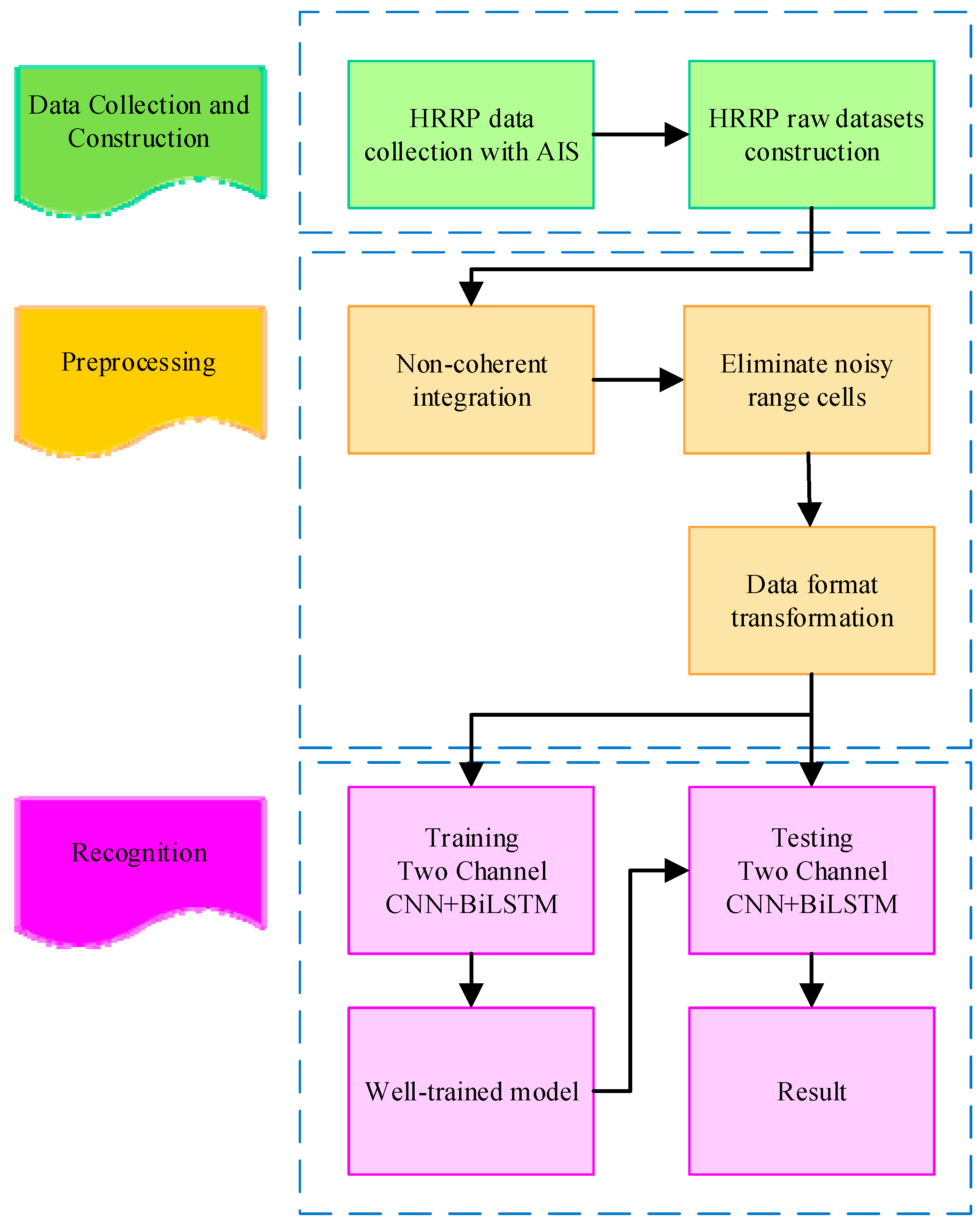
We conducted experiments on the HRRP dataset to evaluate the effectiveness of the proposed approach. The experiments are divided into two parts according to the computing platforms.

The first parts of the test were performed on the CPU of a notebook equipped with Intel^®Core™ i5-7300HQ CPU @ 2.50 GHz × 2, 16 GB RAM and NVIDIA GeForce GTX 1050 GPU. The software was programmed using Python 3.6 and mainly based on the deep-learning framework TensorFlow 1.9.0 + Keras 2.2.4.

The second parts of the test were performed on Colaboratory (or Colab) GPU resources provided by Google. The free computing resources of Colab change over time to adapt to fluctuations in demand, overall growth and other factors. Colab allows people to write and execute an arbitrary Python code through a browser. The GPUs available in Colab typically include NVIDIA K80s, T4s, P4s and P100s, and the available types change over time. Selecting the type of the GPU that can be connected in Colab at any given time is not possible [18].

Experiments 1 to 3 were executed on the CPU platform. According to various condition settings, the parameter settings for which LSTM or BiLSTM exhibited a high recognition accuracy were determined. Based on the results of Experiments 1–3, Experiment 4 was performed to determine how to concatenate a two-channel CNN with LSTM or BiLSTM. Then, the designed deep neural network was executed on the CPU and GPU platforms to determine the highest recognition accuracy according to various condition settings and analyze the time cost.

5.1. HRRP Dataset

The radar HRRP ship target dataset was prepared using the ship information collected by radar and an automatic identification system (AIS). This dataset contains a large amount of HRRP data, which were collected from real-life scenarios [15].

Table 1. Ship types and data chips distribution.

Ship Types	Original Chips	Valid Chips
Alpha	66,792	66,746
Beta	40,346	40,344
Gamma	21,697	21,680
Delta	53,082	53,082
Epsilon	11,493	11,493
Zeta	14,200	14,200
Total	207,610	207,545

lists the distribution of the chips data of six ship types and reveals that this dataset was imbalanced. The original dataset had the data of 207,610 chips, and the invalid chips data with echo values of 0 were removed. The number of valid data items after selection was 207,545. The six types of ships in the study are named Alpha, Beta, Gamma, Delta, Epsilon and Zeta (Figure 8). The HRRP dataset exhibits three essential properties, namely reality, diversity and large scale. Figure 9a,c display two ship types. Figure 9b,d show that each color trajectory represents different continuous data collected. These data indicate that the ship data collected are diverse and include various ranges and azimuths.

5.2. Experiments

The split rate of the dataset was divided into the training set and the test set and affected the recognition accuracy of the training model. It is well known that the neural networks usually perform well with a lot of training data. According to our previous study [15], we have used different split ratios of the training and test datasets in the experiments, which also confirm this result. Therefore, we will no longer discuss the split ratio of training and test datasets in this study. In these experiments, all HRRP data were randomly divided at a ratio of 7:3, which resulted in 145,282 samples of training dataset and 62,263 samples of test dataset. In the training process, 20% of the training dataset was used as the validation dataset, and the accuracy of the validation dataset was used to evaluate the quality of the model. The initial learning rate was set to 0.0001, and the batch size was 300.

Experiment 1: The number of layers in LSTM was fixed as one layer, and the number of neurons was increased in this layer for experiments.

Table 2. Network performance of single-layer LSTM and BiLSTM architecture.

Number of Neuros	#100		#300		#500
Network Arch.	LSTM	BiLSTM	LSTM	BiLSTM	LSTM	BiLSTM
Parameters	41,406	82,806	364,206	728,406	1,007,006	2,014,006
Training Time(s)	1333	2826	5907	12,293	12,986	27,702
Valid. Loss	3.85%	3.27%	3.21%	2.75%	2.63%	2.53%
Valid. Accuracy	98.56%	98.85%	99.18%	99.03%	99.09%	99.21%
Test Time(s)	7.43	13.37	19.66	37.46	43.03	89.11
Test Loss	3.91%	3.91%	3.42%	3.10%	3.81%	3.12%
Test Accuracy	98.63%	98.64%	98.77%	98.95%	98.81%	98.96%

lists that the overall test accuracy was between 98% and 99%. When the number of hidden layer neurons gradually increased, the accuracy also increased. When the number of neurons was 300, the test accuracy was 98.77%. As the number of neurons increased to 500, the increase in test accuracy was marginal. Therefore, an increase in neurons improved accuracy. Although the optimal accuracy was achieved when the number of neurons was approximately 500, the increment was not high. For similar experiments with BiLSTM, when the number of neurons was 500, the highest test accuracy of 98.96% was achieved.

Experiment 2: The previous experiment demonstrated that as the number of neurons increased, the test accuracy increased. Therefore, the second experiment was performed to investigate whether the use of multilayer LSTM affects the accuracy of the network. Here, 300 neurons were evenly distributed in two, three and four layers of LSTM.

Table 3. Network performance of a multilayer LSTM and BiLSTM architecture with the total number of multilayer neurons fixed at 300.

Number of Neuros	2 Layers (#150 × 2)		3 Layers (#100 × 3)		4 Layers (#75 × 4)
Network Arch.	LSTM	BiLSTM	LSTM	BiLSTM	LSTM	BiLSTM
Parameters	272,706	725,406	202,206	564,406	159,456	453,906
Training Time(s)	2475	17,051	3856	16,358	7692	17,321
Valid. Loss	2.08%	2.56%	2.11%	2.76%	2.53%	2.86%
Valid. Accuracy	99.23%	99.13%	99.24%	99.11%	99.07%	99.08%
Test Time(s)	25.57	58.79	27.48	66.17	30.52	73.07
Test Loss	3.61%	3.15%	3.51%	2.84%	3.76%	3.36%
Test Accuracy	98.72%	98.95%	98.85%	99.06%	98.73%	98.89%

indicates that the test accuracy did not increase significantly as the number of LSTM layers increased (the number of neurons in each layer decreased). Multiple LSTM layers required more test time, which is not conducive to practical applications. When the number of neurons was 100 and the three LSTM layers were used, the optimal accuracy of 98.85% was achieved. Furthermore, the training time of a single-layer LSTM of 300 was longer than that of a single-layer LSTM. Therefore, an overly complex architecture does not considerably improve the test accuracy but increases the time cost. Experiments were conducted in a similar manner with BiLSTM. When the number of neurons was 100 and LSTM was three layered, the optimal test accuracy of 99.06% was achieved.

Experiment 3: The previous two experiments revealed that fixing the total number of neurons and increasing the number of LSTM layers did not improve the accuracy considerably. Although Experiment 1 revealed that the optimal test accuracy was achieved for approximately 500 neurons, the benefit was not substantially higher than that for 300 neurons for various numbers of layers. In Experiment 3, the number of LSTM layers was increased under a fixed 300 neurons in each layer.

Table 4. Network performance of the multilayer LSTM and BiLSTM architecture with 300 neurons per layer.

Number of Neuros	2 Layers (#300 × 2)		3 Layers (#300 × 3)		4 Layers (#300 × 4)
Network Arch.	LSTM	BiLSTM	LSTM	BiLSTM	LSTM	BiLSTM
Parameters	1,085,406	2,890,806	1,806,606	5,053,206	2,527,806	7,215,606
Training Time(s)	16,858	47,258	27,367	80,265	39,159	113,456
Valid. Loss	2.63%	2.60%	3.19%	2.68%	2.75%	3.26%
Valid. Accuracy	99.12%	99.12%	99.11%	99.05%	99.15%	99.07%
Test Time(s)	55.75	149.01	92.52	261.73	261.59	367.85
Test Loss	3.59%	2.87%	3.52%	3.95%	4.14%	3.46%
Test Accuracy	98.83%	99.09%	98.92%	98.72%	98.79%	98.96%

displays that the highest test accuracy was obtained when the number of neurons in each layer was 300. The test accuracy did not increase with the number of LSTM layers. Overly complex architecture does not improve the test accuracy but increases time constraints. However, Experiments 3 and 4 revealed that with two LSTM layers, the network with more neurons in each layer had a higher test accuracy. Too many LSTM layers resulted in decreased test accuracy.

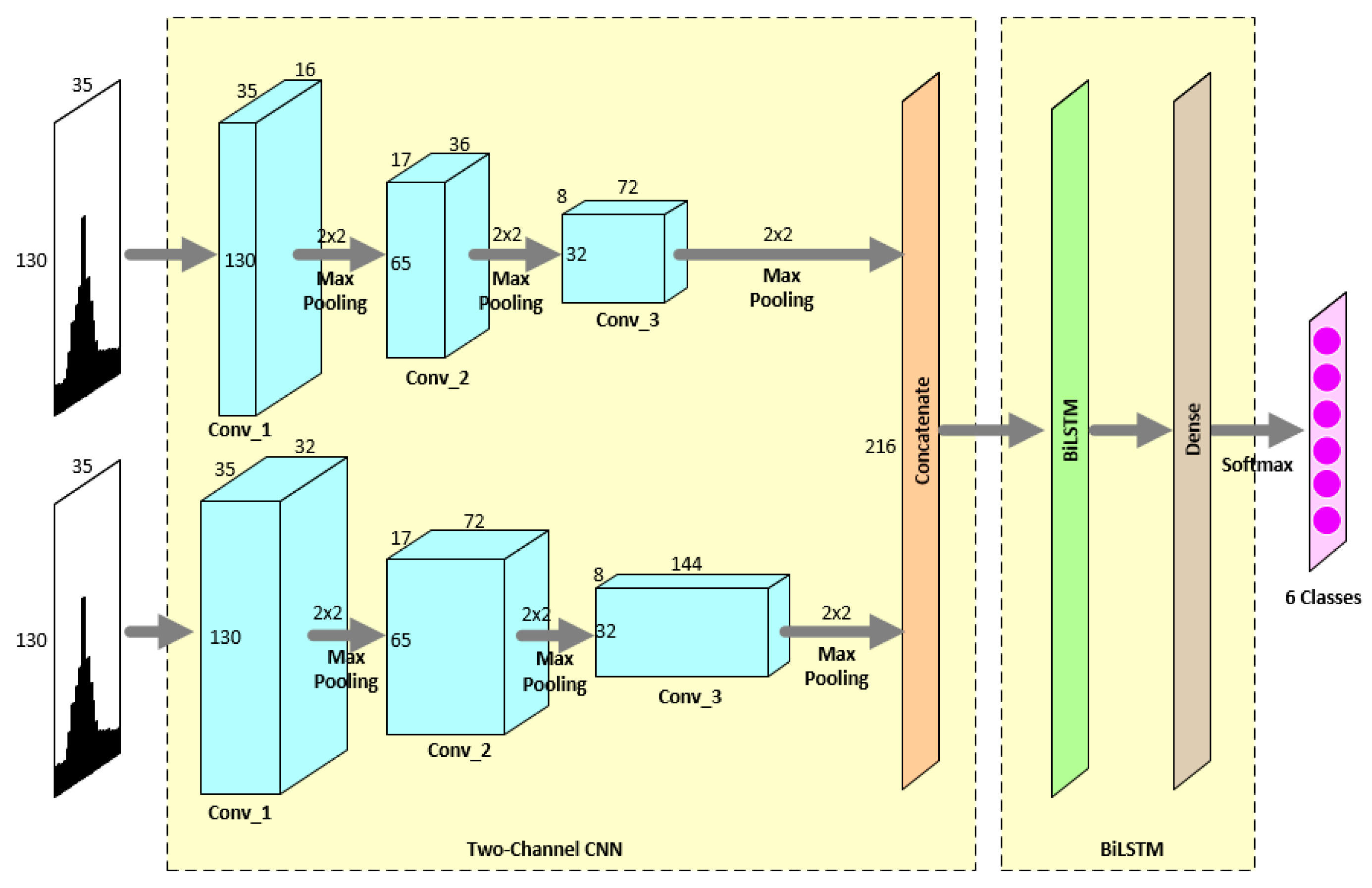
Experiment 4: The experiments were first simulated on the CPU to determine a satisfactory concatenated network structure. The aforementioned experiments indicated that optimal results were obtained when two layers of LSTM were used and the number of neurons in each layer was 300. Therefore, we used a two-channel CNN to concatenate with LSTM and BiLSTM, respectively. First, the number of neurons in each LSTM layer was set to 300, and the number of LSTM layers was fixed to two. Then, a test accuracy of 99.15% was obtained by concatenating the two-channel CNNs with the two-layer LSTM in 160.5 s, which is high. Because the proposed network structure is complex, we speculate that an overly complex network cannot considerably improve recognition accuracy. As displayed in

Table 5. Network performance of the two-channel CNN concatenated with a single-layer LSTM architecture.

Number of Neuros	#100		#300		#500
Computing Env.	CPU	GPU	CPU	GPU	CPU	GPU
Parameters	577,970	577,970	1,591,170	1,591,170	2,924,370	2,924,370
Training Time(s)	62,631	3115	71,422	3330	79,112	3797
Valid. Loss	2.93%	2.50%	2.54%	2.55%	2.45%	2.54%
Valid. Accuracy	99.04%	99.25%	99.17%	99.23%	99.22%	99.23%
Test Time(s)	133.66	11.24	149.07	12.33	177.03	13.22
Test Loss	3.08%	2.81%	2.70%	2.86%	2.68%	2.62%
Test Accuracy	98.96%	99.07%	99.11%	99.12%	99.17%	99.16%

, we concatenated the two-channel CNN with one-layer LSTM and obtained a test accuracy of 99.11%. This accuracy is not considerably lower than that for concatenating two-layer LSTM. A similar experiment was conducted for the BiLSTM experiment. A test accuracy of 99.21% was obtained when a two-channel CNN was concatenated with a two-layer BiLSTM. When the number of BiLSTM layers was set to 1, the test accuracy was 99.24%. For the final experiment, we concatenated a two-channel CNN with one-layer LSTM and BiLSTM. As presented in

Table 6. Network performance of the two-channel CNN concatenated with a single-layer BiLSTM architecture.

Number of Neuros	#100		#300		#500
Computing Env.	CPU	GPU	CPU	GPU	CPU	GPU
Parameters	964,570	964,570	2,990,970	2,990,970	5,657,370	5,657,370
Training Time(s)	56,763	3251	71,846	4813	90,827	4545
Valid. Loss	2.76%	2.35%	2.44%	2.47%	3.26%	2.95%
Valid. Accuracy	99.23%	99.23%	99.27%	99.28%	99.26%	99.25%
Test Time(s)	139.65	13.44	179.79	18.38	227.37	17.54
Test Loss	3.19%	2.54%	2.73%	2.90%	3.32%	2.81%
Test Accuracy	99.14%	99.21%	99.24%	99.25%	99.20%	99.18%

, when the number of neurons was 300, the two-channel CNN concatenated with one-layer BiLSTM achieved the optimal test accuracy of 99.24%.

Table 5 and Table 6 indicate that the proposed model exhibited a superior recognition accuracy, regardless of whether it was concatenated with LSTM or BiLSTM. The execution results on the GPU differed slightly from those of the CPU. However, reproduction of the accuracy was difficult despite repeated tests. However, the difference in the test result when using the GPU was less than 0.1%. Studies have revealed that this phenomenon could be attributed to the complex set of GPU libraries, some of which may introduce their own randomness and prevent accurate reproduction of the results. Regarding time cost evaluation, we analyzed the results from various execution platforms. Because our model is complex, the data of 62,263 chips of HRRP ship data were tested in 178.65 s when executed on the CPU, which indicates that approximately 2.87 ms are required to recognize a chip of HRRP ship data. When executed on the GPU, testing was completed in 18.38 s, which indicates that approximately 0.30 ms are required to recognize a chip of HRRP ship data. For radar systems, a dwell time is typically 10–20 ms. Therefore, the time required for the proposed deep-learning model for radar systems is feasible. System-on-chips equipped with GPUs can be used in radar systems.

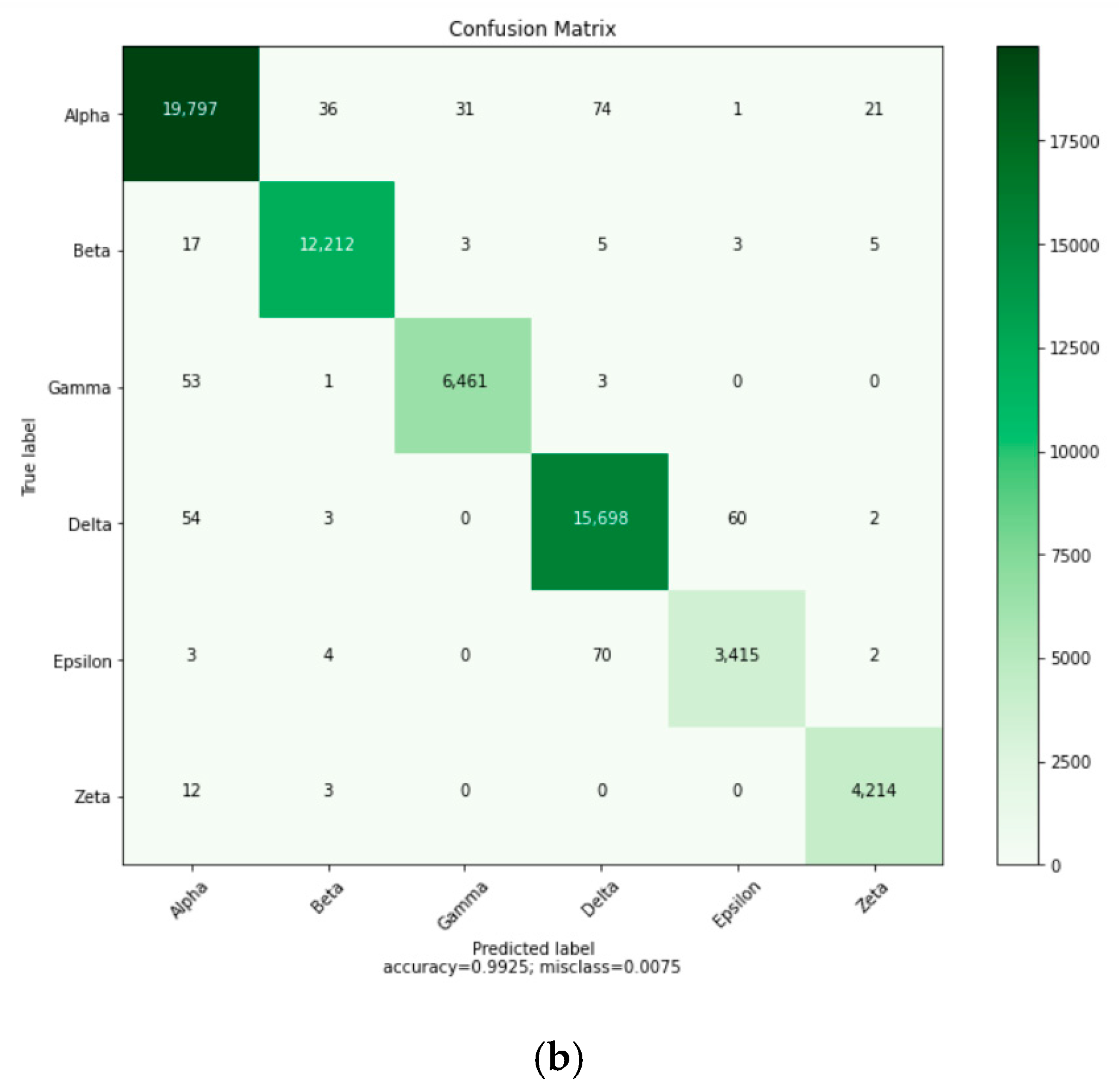
Figure 10 displays the confusion matrix of the recognition results using the proposed two-channel CNN concatenated with BiLSTM model. Figure 10a presents the results for the model running on the CPU, and Figure 10b displays the results for the model running on the GPU. The results of the confusion matrix indicate that ships with similar HRRPs do have higher chances of being confused.

For the CPU model, Delta ships were incorrectly predicted as Alpha ships 59 times; Alpha ships were incorrectly predicted as Delta ships 69 times; Epsilon ships were incorrectly predicted as Delta ships in 94 cases; Delta ships were incorrectly predicted as Epsilon ships in 41 cases.

For the GPU model, Delta ships were incorrectly predicted as Alpha ships 54 times; Alpha ships were incorrectly predicted as Delta ships 74 times; Epsilon ships were incorrectly predicted as Delta ships in 70 cases; Delta ships were incorrectly predicted as Epsilon ships in 60 cases.

From the analysis of the aforementioned results, although the confusion matrices of the data in different environments were not the same, the results of ships easily confused with each other were consistent and with no violation.

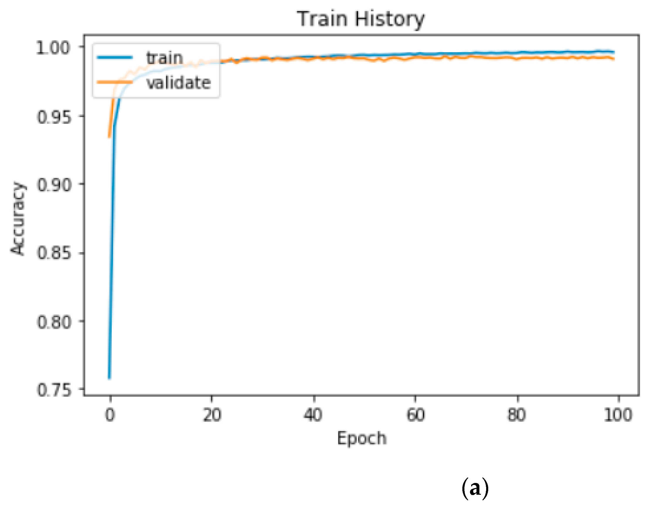
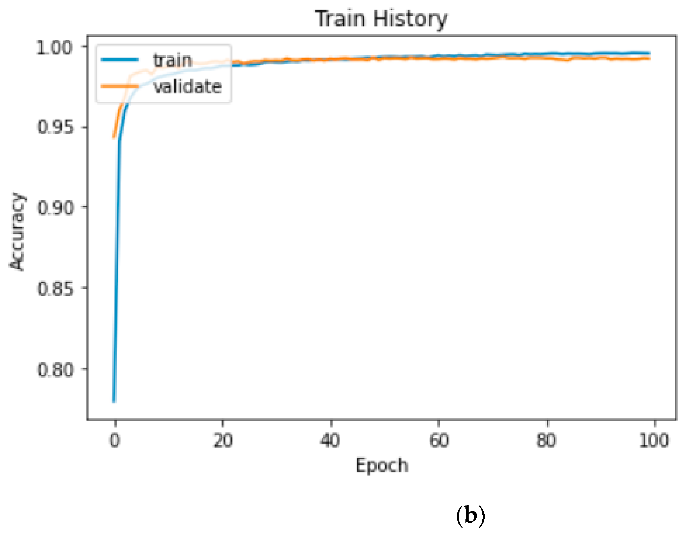
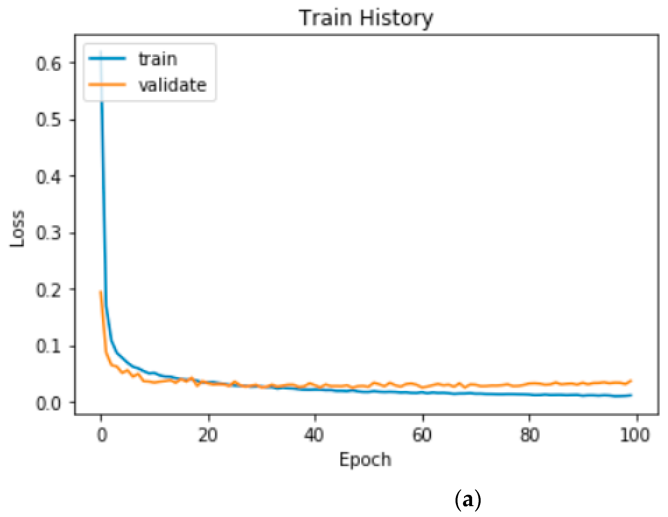
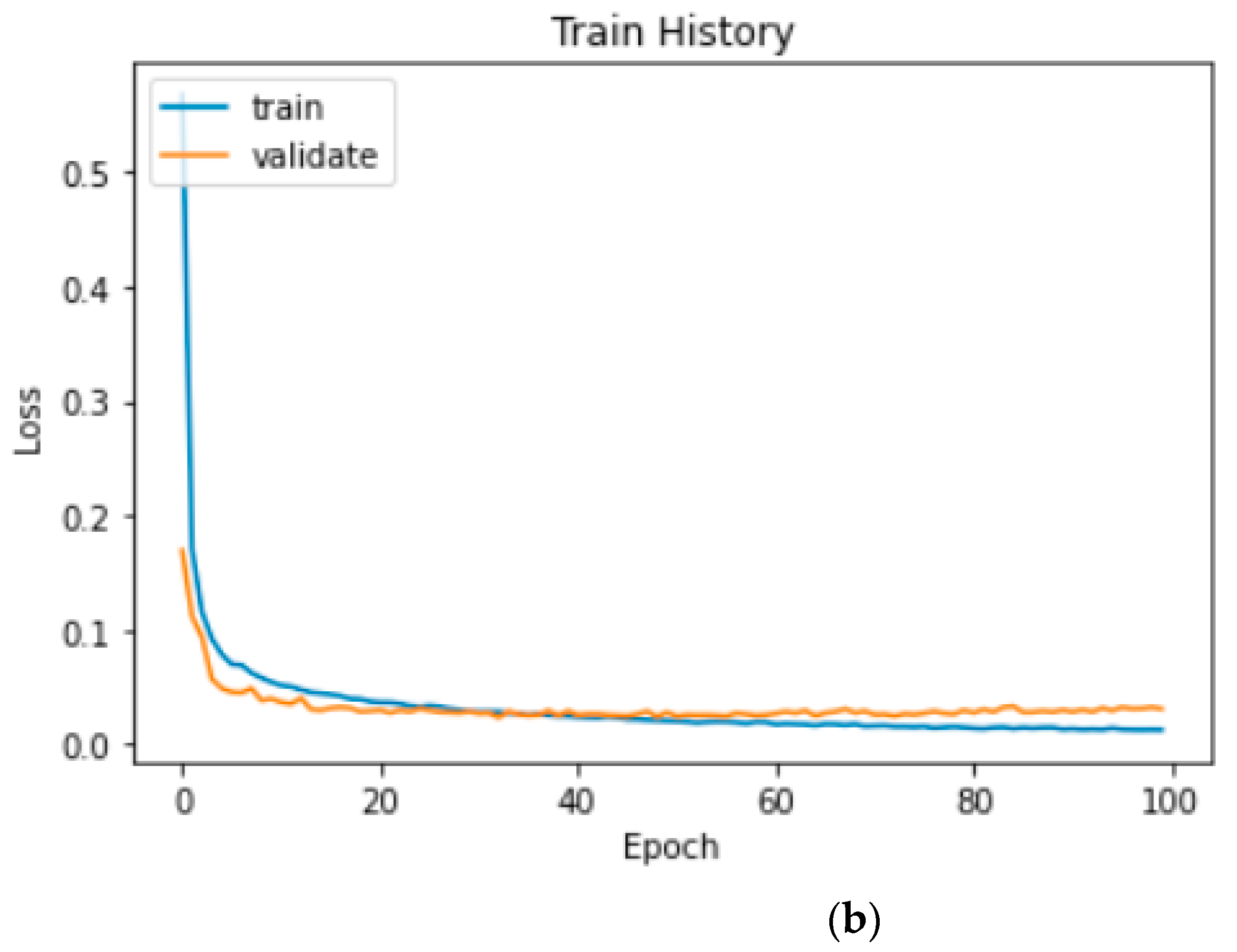
Figure 11 illustrates the recognition accuracy curves of the proposed two-channel CNN–BiLSTM model. Figure 11a presents the results for the model running on the CPU, and Figure 10b displays the confusion matrix for the model running on the GPU. Figure 12 illustrates the loss curve of the proposed two-channel CNN–BiLSTM model. Figure 11a displays the recognition accuracy curve of the model running on the CPU, and Figure 11b displays the recognition accuracy of the model running on the GPU. Figure 11 and Figure 12 indicate that the accuracy of the validation set did not increase considerably after approximately 60 epochs, and the loss of the validation set did not decrease considerably after approximately 60 epochs. According to our experimental records, when running on the CPU, the highest accuracy of 99.27% was obtained in 63 epochs in the validation set, and the loss in the validation set was 2.44%. When running on the GPU, the accuracy of the validation set reached the highest accuracy of 99.29% in 73 epochs, and the loss of the validation set was 2.47%.

Finally, the results were compared with some well-known network architectures. As displayed in

Table 7. Network performance of all the experiments conducted on the constructed HRRP dataset.

Approach	Description	Recognition Accuracy
LeNet	LeNet	99.05%
AlexNet	AlexNet	98.94%
ZFNet	ZFNet	98.85%
VGG-16	VGG-16	98.53%
LSTM	3-layer LSTM with 300 neurons per layer	98.92%
BiLSTM	2-layer BiLSTM with 300 neurons per layer	99.09%
2 CNN+LSTM	Two-channel CNN concatenated with LSTM	99.17%
2 LeNet+BiLSTM	Two-channel LeNet concatenated with BiLSTM	99.09%
2 AlexNet+BiLSTM	Two-channel AlexNet concatenated with BiLSTM	98.97%
2 CNN+BiLSTM	Two-channel CNN concatenated with BiLSTM	99.25%

, we summarized all the experiments performed on the same HRRP dataset and conducted with the same training and validation datasets. Comparisons of LeNet, AlexNet, ZFNet and VGG16 revealed that deeper networks may not achieve superior results. However, deeper layers exhibited superior results in the VGG architecture. Table 7 indicates that the proposed approach outperformed the two-channel LeNet and AlexNet.

5.3. Comparison with State-of-the-Art Approaches

Table 8. Comparison of for HRRP recognition performance for various approaches.

Approach	Dataset	Description	Recognition Accuracy (%)	Year
[10]	Simulation data	CNN-MatConvNet	93.90%	2017
[12]	Simulation data	CNN	94.30%	2019
[13]	Simulation data	CNN-ELM	99.50%	2019
[14]	Simulation data	CNN-BiRNN	93.30%	2020
[15]	Our real-life data	3Conv+2FullyConnect CNN	99.20%	2020
2 CNN+BiLSTM	Our real-life data	Two-channel CNN+BiLSTM	99.25%	2021

Bold values indicate the optimal performance with real-life data.

summarizes experimental results in published papers using deep-learning approaches. In Table 8, the datasets in [10,12,13,14] are established in a simulated manner, and the datasets used in this paper are the data collected from real-life situations.

Karabayır et al. [10] proposed stacking a one-dimensional HRRP data by simply copying to obtain an enhanced two-dimensional gray-scale image and directly feeding the one-dimensional HRRP into the neural network. The difference in the recognition rate was nonsignificant and was between 98% and 99%. Zhang et al. [13] proposed a CNN–ELM network for ship HRRP target recognition. In the experiment, CNN–ELM achieved a recognition rate of 99.50%. Wan et al. [14] proposed a CNN–BiRNN-based method to identify aircraft HRRP and achieved an optimal recognition effect of 93.30%. Chen et al. [15] proposed a two-dimensional HRRP data format and applied CNN to HRRP for ship target recognition. Experiments revealed that the CNN exhibited an excellent recognition rate of 99.20%.

Unlike the data collected under the real-life environment in this study, most studies have simulated HRRP. Table 8 indicates that the studies using deep neural networks to identify ships have exhibited excellent accuracy. Furthermore, the proposed approach is comparable to the other state-of-the-art HRRP target recognition approaches.

6. Conclusions

Radar HRRP target recognition is a critical target recognition problem in the RATR field. In the past, most of the radar automatic target recognition methods use conventional handcrafted features. These methods require prior knowledge of radar and can only achieve limited effects. In recent years, many deep neural network-based recognition methods have emerged. The use of deep neural networks for radar HRRP target recognition helps to avoid excessive use of artificially designed rules to extract features, and deep learning can automatically obtain the deep features of the target.

This study proposed a deep neural network-based two-channel CNN concatenated with BiLSTM for ship target recognition based on radar HRRP. A two-channel CNN with various filters can dig out more different features. These features can be used as the input to BiLSTM to investigate the spatial relationship of adjacent range cells of HRRPs. BiLSTM is a two-directional timeseries and is highly robust for timeseries data modeling. The BiLSTM model can capture long-distance dependence and obtain superior two-way timing dependence. Therefore, two-way continuous time sequential features of the ship structure—that is, the two-way spatial relationship between adjacent range cells—can be determined.

It can be seen from the experiments with a real-life HRRP dataset of ship targets that the use of a timeseries neural network has good recognition accuracy. BiLSTM is slightly better than LSTM, which indicates that the adjacent structure of ship targets should have continuous relational characteristics, that is, adjacent range cells in HRRP have timeseries features. In addition, it can be seen that the two-directional timeseries features are more discriminative than the one-directional timeseries features. The proposed method is also better than using BiLSTM or LSTM alone. It reveals that the use of two-channel CNN can more effectively extract discriminative deep features.

The results of the proposed approach are comparable to those of other existing state-of-the-art HRRP target recognition approaches. An experimental comparison of CPU and GPU performance was performed, which revealed that on current high-speed GPU computing platforms, the use of complex deep neural networks for radar HRRP target recognition is feasible. The findings of this study can extend HRRP recognition technologies to the applications of coastal surveillance, navigation channel management and military RATR.

References

1. Du, L.; Liu, H.; Bao, Z.; Xing, M. Radar HRRP target recognition based on higher order spectra. IEEE Trans. Signal Process. 2005, 53, 2359–2368. [Google Scholar]
2. Luo, S.; Li, S. Automatic target recognition of radar HRRP based on high order central moments features. J. Electron. (China) 2009, 26, 184–190. [Google Scholar] [CrossRef]
3. Lu, J.; Xi, Z.; Yuan, X.; Yu, G.; Zhang, M. Ship target recognition using high resolution range profiles based on FMT and SVM. In Proceedings of the IEEE CIE International Conference on Radar, Chengdu, China, 24–27 October 2011. [Google Scholar]
4. Zhou, D.; Shen, X.; Liu, Y. Nonlinear subprofile space for radar HRRP recognition. PIER Lett. 2012, 33, 91–100. [Google Scholar] [CrossRef] [Green Version]
5. Feng, B.; Du, L.; Shao, C.; Wang, P.; Liu, H. Radar HRRP target recognition based on robust dictionary learning with small training data size. In Proceedings of the IEEE Radar Conference, Ottawa, ON, Canada, 29 April–3 May 2013. [Google Scholar]
6. Liu, J.; Fang, N.; Xie, Y.J.; Wang, B.F. Multi-scale feature-based fuzzy-support vector machine classification using radar range profiles. IET Radar Sonar Navig. 2016, 10, 370–378. [Google Scholar] [CrossRef]
7. Du, L.; He, H.; Zhao, L.; Wang, P. Noise robust radar HRRP targets recognition based on scatterer matching algorithm. IEEE Sens. J. 2016, 16, 1743–1753. [Google Scholar] [CrossRef]
8. Lundén, J.; Koivunen, V. Deep learning for HRRP-based target recognition in multistatic radar systems. In Proceedings of the IEEE Radar Conference, Philadelphia, PA, USA, 2–6 May 2016; pp. 1–6. [Google Scholar]
9. Yuan, L. A time-frequency feature fusion algorithm based on neural network for HRRP. Prog. Electromagn. Res. 2017, 55, 63–71. [Google Scholar] [CrossRef] [Green Version]
10. Karabayır, O.; Yücedağ, O.M.; Kartal, M.Z.; Serim, H.A. Convolutional neural networks-based ship target recognition using high resolution range profiles. In Proceedings of the International Radar Symposium, Prague, Czech Republic, 28–30 June 2017. [Google Scholar]
11. Liao, K.; Si, J.; Zhu, F.; He, X. Radar HRRP Target Recognition Based on Concatenated Deep Neural Networks. IEEE Access 2018, 6, 29211–29218. [Google Scholar] [CrossRef]
12. Song, J.; Wang, Y.; Chen, W.; Li, Y.; Wang, J. Radar HRRP recognition based on CNN. IEEE IET 2019, 7766–7769. [Google Scholar] [CrossRef]
13. Zhang, Q.; Lu, J.; Liu, T.; Zhang, P.; Liu, Q. Ship HRRP Target Recognition Based on CNN and ELM. In Proceedings of the IEEE ICECTT Conference, Guilin, China, 26–28 April 2019. [Google Scholar]
14. Wan, J.; Chen, B.; Liu, Y.; Yuan, Y.; Liu, H.; Jin, L. Recognizing the HRRP by Combining CNN and BiRNN with Attention Mechanism. IEEE Access 2020, 8, 20828–20837. [Google Scholar] [CrossRef]
15. Chen, T.-P.; Lin, C.-L.; Fan, K.-C.; Lin, W.-Y.; Kao, C.-W. Apply convolutional neural network to radar automatic target recognition based on real-life radar high-resolution range profile of ship target. In Proceedings of the CVGIP, Hsinchu, Taiwan, 16–18 August 2020. [Google Scholar]
16. LeCun, Y.; Bengio, Y. Convolutional networks for images, speech, and time series. In The Handbook of Brain Theory and Neural Networks; Arbib, M.A., Ed.; MIT Press: Cambridge, MA, USA, 1995. [Google Scholar]
17. Hochreiter, S.; Schmidhuber, J. Long short-term memory. Neural Comput. 1997, 8, 1735–1780. [Google Scholar] [CrossRef] [PubMed]
18. Colaboratory Frequently Questions. Available online: https://research.google.com/colaboratory/faq.html (accessed on 13 November 2020).
Figure 1. Block diagram of the proposed approach.
Remotesensing 13 01259 g001
Figure 2. Schematic of the two-dimensional binary map high-resolution range profile (HRRP) data format.
Remotesensing 13 01259 g002
Figure 3. Simple convolutional neural network (CNN).
Remotesensing 13 01259 g003
Figure 4. Architecture of the long short-term memory (LSTM) cell.
Remotesensing 13 01259 g004
Figure 5. Architecture of bidirectional long short-term memory (BiLSTM).
Remotesensing 13 01259 g005
Figure 6. Proposed two-channel CNN–BiLSTM model.
Remotesensing 13 01259 g006
Figure 7. Architecture of the proposed two-channel CNN.
Remotesensing 13 01259 g007
Figure 8. Six ship types and their HRRPs.
Remotesensing 13 01259 g008
Figure 9. Examples of automatic identification system (AIS) information and trajectories of the collected ships. (a,c) display the pictures of two ships. (b,d) display the trajectories of the two ships displayed in (a,c), respectively.
Remotesensing 13 01259 g009
Figure 10. Confusion matrix of the proposed two-channel CNN–BiLSTM model: (a) run on the CPU and (b) run on the GPU.
Remotesensing 13 01259 g010aRemotesensing 13 01259 g010b
Figure 11. Recognition accuracy curve of the proposed two-channel CNN–BiLSTM model: (a) run on the CPU and (b) run on the GPU.
Remotesensing 13 01259 g011aRemotesensing 13 01259 g011b
Figure 12. Loss curve of the proposed two-channel CNN–BiLSTM model: (a) run on the CPU and (b) run on the GPU.
Remotesensing 13 01259 g012aRemotesensing 13 01259 g012b