
Photogrammetric Digital Surface Model Reconstruction in Extreme Low-Light Environments


1
Department of Engineering and Architecture, University of Parma, 43124 Parma, Italy
2
Centre for Geotechnical Science and Engineering, University of Newcastle, Callaghan 2308, Australia
*
Author to whom correspondence should be addressed.
Remote Sens. 2021, 13(7), 1261; https://doi.org/10.3390/rs13071261
Submission received: 5 March 2021
/
Revised: 18 March 2021
/
Accepted: 22 March 2021
/
Published: 26 March 2021
(This article belongs to the Special Issue 3D Point Clouds in Rock Mechanics Applications)
Abstract
:Digital surface models (DSM) have become one of the main sources of geometrical information for a broad range of applications. Image-based systems typically rely on passive sensors which can represent a strong limitation in several survey activities (e.g., night-time monitoring, underground survey and night surveillance). However, recent progresses in sensor technology allow very high sensitivity which drastically improves low-light image quality by applying innovative noise reduction techniques. This work focuses on the performances of night-time photogrammetric systems devoted to the monitoring of rock slopes. The study investigates the application of different camera settings and their reliability to produce accurate DSM. A total of 672 stereo-pairs acquired with high-sensitivity cameras (Nikon D800 and D810) at three different testing sites were considered. The dataset includes different camera configurations (ISO speed, shutter speed, aperture and image under-/over-exposure). The use of image quality assessment (IQA) methods to evaluate the quality of the images prior to the 3D reconstruction is investigated. The results show that modern high-sensitivity cameras allow the reconstruction of accurate DSM in an extreme low-light environment and, exploiting the correct camera setup, achieving comparable results to daylight acquisitions. This makes imaging sensors extremely versatile for monitoring applications at generally low costs.
1. Introduction
Digital surface models (DSM) have become one of the main sources of geometrical information for many different applications. Recent substantial improvements in processing hardware and software allow obtaining a detailed three-dimensional (3D) reconstruction of generic objects with millions (and sometimes billions) of 3D point coordinates. The final product of a DSM reconstruction, which can be a point cloud, a raster representation of heights or distances from the observer, a 3D triangular mesh (triangulated irregular network—TIN) or a more complex structured surface (quad- or poly-mesh, non-uniform rational B-spline (NURBS), etc.), can be obtained with several different techniques [1,2,3,4].
In recent years, leveraging on innovative algorithms that have automated the entire processing pipeline, image-based techniques, along with LiDAR (light detection and ranging), have become the most used approach for close-range and proximity surveys. In these contexts, image-based systems have become the preferable solution for many applications due to the low cost of instrumentation, their portability and usability and the availability of free or low-cost processing software (i.e., less than five thousand dollars). However, image-based systems are typically based on a passive sensor, i.e., the device used to acquire image data relies on external light sources (e.g., the sun or an artificial illuminator), and an adequate illumination of the object is required to obtain accurate results. The problem is overcome by performing the image acquisition in a controlled environment, or in an environment with direct sunlight. Perfect conditions are hardly achievable during several survey activities such as night-time monitoring [5,6], traffic accident reconstruction [7], underwater [8,9] and underground [10,11] photogrammetry and night surveillance [12,13], to name a few.
Nicolae et al. [14] reported several case studies concerning 3D reconstruction of museum artefacts, where very long exposure times (and narrow aperture) were considered: the use of artificial light, in that case, would have produced strong shades and reflection, preventing an accurate object reconstruction. In Pappa et al. [15], long exposures combined with a dot projector were required to reconstruct the shape of large membrane reflectors and other space structures.
Several recent digital single lens reflex (DSLR) cameras are equipped with full frame sensors, which are less prone to noise effects [16], with very high sensitivity that also allow capturing images in exceptional low-light environments. For instance, the Canon ME20F-SH camcorder can reach a remarkable ISO of over 4 million and supports infrared filming. The Nikon D5 can shoot a maximum ISO of up to 3.28 million. The Canon 5D mark IV reaches an ISO of 102,400 and the Nikon D810 an ISO of 51,200. The ISO value expresses the sensitivity of the sensor to the incoming light. For digital cameras, different sensitivities can be implemented, amplifying the signal from the sensor [17] before and/or after analog-to-digital conversion (ADC). High ISO values increase the light sensitivity, but also result in noisy and grainy images, associated with the amplified image noise. Some cameras are equipped with a high ISO noise reduction (HI-NR) function, which reduces the graininess of the image acquired with a high amplification level by post-processing the image data [18]. However, such operation generally results in a loss of sharpness. More recently, the use of machine and deep learning algorithms to enhance image quality in low-light conditions has also been investigated (e.g., [19]).
The light energy collected by the sensor can be increased in an imaging system operating on two parameters: exposure, i.e., the period the sensor is exposed to light and absorbs radiant energy, and aperture, i.e., the area through which the radiant flux travels inside the optics, which can usually be controlled by a device such as a diaphragm.
The use of longer exposure times allows collecting more radiant energy but might produce blurred images if a relative motion between the object and observer cannot be prevented. Additionally, with long exposures, there exists the potential for the camera sensor to heat up, which can result in noisy images. The image is affected by a random pattern of odd colored pixels (commonly referred to as “hot pixels”) which reduces the quality of the image itself. In many DSLR cameras, a long exposure noise reduction (LE-NR) feature might reduce the presence of hot pixels, operating a dark frame subtraction [20]. However, as with HI-NR, the result might not be optimal and, after the LE-NR application, the resulting image might have a lower level of detail or be affected by additional artefacts.
An increase in the optics’ aperture allows collecting more radiant energy but can also generate a shorter depth of field, which might produce unfocused elements in the image. Moreover, optical aberrations can occur, affecting the actual image resolution (and sharpness): blurs might occur with narrow aperture diffraction, and while a wide aperture defocuses the blurs, the image can still be affected by vignetting and astigmatism.
To the authors’ best knowledge, very few quantitative analyses [21] can be found in the literature focusing on the photogrammetric accuracy achievable with different exposure setups (i.e., varying appropriately ISO speed, shutter speed and aperture). Certainly, as far as daylight photogrammetry is concerned, a fairly easy setup can be obtained using intermediate apertures (f/5.6 or f/8), a low ISO speed (200 or lower) and a fast shutter speed (shorter than 1/30 s), granting an optimal image quality. However, some open issues remain on the optimal settings required to achieve the highest photogrammetric accuracy for low-light environments.
This work focuses on the analysis of the performances of low-light and night-time images. The study explores different settings of a DSLR camera during night-time acquisitions accounting for different values of ISO, aperture and time of exposure. Their effect on image quality and reliability to produce accurate DSM for change detection analyses is investigated. The cameras considered in this study are a Nikon D800 and a Nikon D810. The investigation of the performance of different cameras/sensors/optics is out of the scope of the current research. In particular, the current study aims at identifying the optimal setup for “extreme” low-light acquisition in fixed photogrammetric systems for accurate rock slope monitoring applications, where the possibility of operating the system also during the night-time would considerably extend the analysis of the phenomena (usually a rockfall event). In this case, the adjective “extreme” low-light refers to a condition where, during the night-time, artificial lighting is totally missing. Recently, on-site permanent installations of cameras for monitoring purposes have received increased attention in the scientific literature [22,23,24,25,26,27,28] and by the industry. The focus of this paper is on the influence of different camera settings using current mid-level DSLR cameras (Nikon D800 and D810). It should be pointed out that several newer models have a wider native ISO speed (e.g., the Nikon D850 has a maximum native ISO of 25,600, 2 stops higher than the Nikon D800 which allows a native ISO of up to 6400, and the Nikon D6 reaches a native ISO of 102,400, which is 4 times higher) and would probably perform better than the cameras considered in the paper.
In this context, it is also important for the system data to be reliably collected at each acquisition period. For this reason, the paper also investigates the possibility of implementing image quality assessment (IQA) methods to check each single image right after the acquisition in order to predict if an accurate reconstruction can be obtained at the end of the photogrammetric processing pipeline. It will be shown that, considering the general purposes of IQA methods, such approach requires a careful tuning of the procedure and, in some cases, can provide different performances depending on peculiar characteristics of the acquisition. The development, however, of a specific night-time IQA method to provide a more general and robust solution to the problem is out of the scope of the present work.
2. Materials and Methods
2.1. Description of Test Sites
Images acquired by three fixed terrestrial monitoring systems were considered in this paper. One system, thoroughly described in [29], was installed in front of an artificially excavated rock face in a surface mine site in Australia, while the other two were set up in front of two natural rock slopes in Italy.
The Australian site (indicated as Site A—Figure 1a) is located in an open cut coal mine in the Hunter Valley, 15 kilometres south of Singleton (New South Wales—Australia). The monitored rock slope (i.e., highwall) is ca. 60 m wide and 47 m tall with a ground sampling distance (GSD) of ca. 8.2 mm. The slope is composed of horizontally bedded layers of sandstone, claystone, mudstone and coal. The rock face is around 70° deep and presents two joint sets of discontinuities whose intersection with the rock face can produce significant wedge sliding instabilities. In particular, blocks detaching from the massive layer of sandstone at the center of the surface can represent an important safety issue for working personnel, equipment and machineries located at the bottom of the wall. The system, specifically developed for the monitoring of sub-vertical rock surfaces in mine environments and the assessment of the spatial–temporal occurrence and magnitude of rock instability events, consists of two stand-alone units (see Section 2.2 for details). The camera stations were set up in a slightly convergent pose to ensure maximum overlap.
The second site (Site B—Figure 1b) is a peculiar geological formation near Reggio Emilia (north of Italy): the south crag of the Pietra di Bismantova (literally Stone of Bismantova). The surveyed outcrop is approximately 100 × 70 m2 and is composed of yellowish calcarenite over a marl basement. The location is a renowned tourist destination for both climbers and trekkers, and the setup of the fixed photogrammetric system was allowed only at late afternoon with the requirement of removal before the following morning. One-night acquisition only was therefore considered for test Site B. The images were acquired from an object distance of approximately 245 m, resulting in a GSD between ca. 13.2 and 14.1 mm, and a block configuration similar to the one of Site A.
The third series of tests was conducted on an exposed rock surface of the cliff of Leverogne (named Site C—Figure 1c) in the Valle D’Aosta region (Italy). The rock wall is about 90 m high and 100 m wide; it is bounded by NW-dipping tectonic mélanges and it lies onto blueschist facies ophiolites. Two acquisition periods were considered and the images were acquired at a distance from the rock wall of approximately 145 m and with a base-length of about 40 m. The site has been previously used by the authors to conduct a preliminary investigation [5]. The initial study showed that, even if the site was specifically identified to eliminate any kind of source of illumination and the environment could have been depicted as very dark (pitch black) by the operator, the images acquired during the night-time were affected by the lights coming from the nearby small town of Arvier (ca. 1 km far from the site), with mild shadows visible on the rock surface.
2.2. Acquisition System
A fixed photogrammetric monitoring system, designed for the monitoring of rockfalls in surface mining [29], was chosen to ensure the highest control and repeatability of the acquisition. The system consists of two stand-alone units that acquire images simultaneously at scheduled times. Each unit includes a camera box, a battery box and a solar panel (Figure 1d). Each camera box contains a DSLR camera, a single-board Raspberry Pi 3 model B (RPi3B) and an uninterruptible power supply (UPS). Each unit is powered by a solar panel and a pack of two batteries stored in the battery box. The Rpi3B has an integrated wireless LAN module that allows connecting the system to an external WI-FI network from where it can be controlled. The user, through the SSH (Secure Shell) protocol, controls all the acquisition parameters, as well as the battery status, temperatures, etc. This allowed the system to be controlled remotely throughout all the experiments. The system is permanently connected to the Internet, and every fifteen minutes, the system clock is updated to have a good synchronization between the two acquisition units. The system is capable of acquiring high-resolution images at predefined times and the user can remotely control all the acquisition parameters (ISO speed, shutter speed, aperture, HI-NR, LE-NR, etc.) by sending commands directly to the acquisition unit or uploading a trigger table (i.e., a table consisting of a list of acquisition times along with the corresponding acquisition parameters). The system installed at Site A (Australia) was equipped with Nikon D810 DSLR cameras and Nikkor f/1.8 50 mm lenses. The systems at Site B and C (Italy) used Nikon D810 DSLR cameras with Sigma f/2.8 90 mm and Nikkor f/1.8 50 mm lenses, respectively. Testing the performance of different sensor/optics combinations is out of the scope of the present work, as stated in the introduction. However, in Site B, it was considered necessary to use lenses with different focal lengths to achieve a comparable GSD with the other two test sites. The most relevant camera parameters are reported in Table 1. The image block parameters for the relevant optics and sites are summarized in Table 2.
2.3. Image Acquisition and Pre-Processing
One of the main objectives of this work is to evaluate the influence of the camera parameters on the final DSM reconstruction accuracy in very low light conditions that can occur in real in situ outdoor applications. Low-light or very low light condition is not a definition per se, but, for outdoor in situ applications during the night-time (when low-light conditions are experienced), the global illumination of the object can vary quite drastically. Some artificial illumination can be received from nearby areas (e.g., machineries and working equipment), the sky can be sufficiently clear and the images can be acquired during full moon, or no light sources of any kind could be available (i.e., the area of interest, if very far from any artificial illumination, and the images are acquired during new moon phases).
In our investigation, the images were acquired during a full-moon phase. For Site A, four datasets were acquired at different periods with different weather conditions: the first sequence of images (identified in the following as A1) was acquired on 23 November 2018 and the sky was cloudy; the second (identified in the following as A2) on 24 November 2018 (partly cloudy); the third (identified in the following as A3) on 19 February 2019 with clear sky; and the fourth (identified in the following as A4) during the night of 20 February with a partly cloudy sky. For Site B, only one acquisition was possible (in the following B1) during the early morning hours of 5 September 2020, with a clear sky. Finally, two datasets were acquired during two consecutive nights for Site C (indicated in the following as C1 and C2, respectively), on 28 and 29 October 2020. During both acquisitions, the sky was very cloudy.
The start time of the acquisition was chosen to ensure a similar (full moon) lighting of the scene for all three sites, even though the slope orientation and inclination are not exactly the same (the rock walls are all sub-vertical but their orientation varies by about 30°). The acquisitions started ca. five hours after moonrise and at least four hours after the sunset.
Time between consecutive shots is needed for image acquisition and transfer; therefore, any acquisition period (ca. 80–120 pairs of images, varying all the exposure parameters) required approximately one and a half hours.
The exposure features of each single shot are quantitatively evaluated by the exposure equation implemented in reflected light meters:
where N is the relative aperture (f-number), t is the exposure time (shutter speed) in seconds, L is the average scene luminance, S is the ISO arithmetic speed as defined in ISO 2720:1974 and K is the reflected light meter calibration constant (12.5 cd/m2 is commonly used by Nikon). Equation (1) can also be rewritten as
Given a specific average scene luminance, which is assumed constant throughout every single experiment (hypothesis not always verified during partly cloudy acquisitions), the same exposure can be obtained with different combinations of ISO speeds, exposure times and apertures.
An absolute exposure value (EV) can be defined as
Note that the absolute exposure value (ISO 100), according to [30,31], of a natural outdoor scene with full-moon light and a clear sky is usually in the range of −3 to −2 (while the EV during the daytime of a cloudy day is usually around +12), while the absolute EV of a scene illuminated by a quarter moon is ca. −6. In Table 3, the absolute exposure values measured during each acquisition are reported.
For sake of simplicity, we prefer to define a relative exposure value (EVr):
where k is an ISO speed constant such that EVr equals zero (EVr = 0) for every combination of acquisition parameters satisfying Equation (2).
To test the influence of different exposures (i.e., considering over- or under- exposed images), all the possible (1-stop) combinations of EVr = 0 and also EVr = −1 (over-exposed) and EVr = +1 (under-exposed) were considered.
For Sites B and C, half-stops (EVr = −0.5 and EVr = +0.5) were also considered during image acquisitions. Apertures considered for the experiments varied between f/2 and f/16 (except for Site B since the optics have a minimum f-number of f/2.8), shutter speeds ranged between 1/8 s and 30 s and ISO speeds ranged between ISO 200 and ISO 25,600 (for Site A, the use of the Nikon D810 allowed acquiring images also with ISO 51,200).
Figure 2 shows samples of the images acquired at EVr = +1, EVr = 0 and EVr = −1 along with their radiometric histogram. The average gray value registered was, respectively, 47, 63 and 109. The histograms show quite clearly that EVr = 0 has the best dynamic range in all the color components, while EVr = 1 presents a more compact histogram (less contrast) and EVr = −1 has some cut-off (over-exposed), especially in the red band.
The ISO speed, aperture and shutter of each image were recorded in the metadata of the image file. The images were transferred to a remote server and further processed. A Wallis filter [32] was applied to all incoming images to enhance and equalize their histogram. Both images, the original and the Wallis-filtered one, were stored on the server.
Wallis filters are commonly used in photogrammetry and remote sensing applications to perform a local adaptive correction of image brightness and contrast. The filter is also useful since it flattens the different exposures to achieve a similar brightness in the images. It can significantly improve feature extraction procedures [33], since the higher (local) dynamic range of the images allows identifying and matching a greater number of features. However, as far as dense image matching is concerned, the effect of the Wallis filter should be verified, since several matching algorithms (e.g., least squares matching—LSM [34]) use the same radiometric model correction.
The data accuracy was assessed by comparing the photogrammetric DSM with a reference 3D model of the slope. A triangulated terrestrial laser scanning (TLS) scan was acquired the day of the installation/acquisition using a Leica C10 at Sites A and B. According to its technical specifications [35], the instrument has a good range (300 m for 90% albedo targets and 134 m for 18% albedo) and an estimated accuracy of 4 mm for single distance measurement and 6 mm for position measurement. It should be noted that, according to the general requirements for accuracy assessment [36], the reference data should be at least three times more precise than the precision expected for the test dataset. According to the precision equation in the normal case of restitution (see, for instance, [37]), the depth accuracy can be estimated by
where Z is the distance from the object, c is the principal distance of the camera (can be approximated with the focal length), B is the base length of the stereo-pair and is the measurement precision of the image coordinates (here optimistically assumed with ±1 pixel [38]). The expected depth accuracy is about 2.6 cm, 5.8 cm and 5.2 cm for Sites A, B and C, respectively. Consequently, for Sites A and B (Figure 3a–b), the TLS measurement precision is considered adequate if compared to the expected accuracy of the fixed photogrammetric system. For Site C (Figure 3c), due to the specific reflective characteristics of the slope, the TLS scan was mostly incomplete and with a high level of noise. Therefore, the data were discarded and the reference DSM was obtained using a DJI Phantom 4 Pro UAV, acquiring a highly redundant (ca. 70 images) high-scale (average distance from the slope was ca. 40 m) image block flying five strips at different altitudes and pointing the camera horizontally (for lower strips) or slightly downward (up to ca. 10°, for higher strips). The image block was oriented using 31 ground control points (GCPs) determined using a Topcon IS200 Total Station. The expected precision of the UAV block, according to Equation (5), is ca. 1.8 cm and the quality of the reference DSM was assessed considering 13 check points uniformly distributed on the slope surface. The average discrepancy between check point coordinates and the DSM is 2.1 cm.
All the reference DSM were considered in a local reference system with a vertical Z axis and X axis oriented parallel to the average slope orientation. The TLS reference DSM were triangulated from the point cloud and consist of ca. 1.25 million vertices (ca. 501 points/m2) for Site A, 525,000 vertices (ca. 424 points/m2) for Site B and ca. one million vertices (403 points/m2) for Site C.
2.4. Image Quality Assessment
The paper aims at investigating the accuracy of DSM obtained in extreme low-light conditions, where no or insufficient artificial light sources are present. For this rationale, the use of a high ISO speed, long exposure times and large apertures may drastically affect the image quality. One of the main goals is, therefore, to identify an optimal exposure setup for such critical conditions and evaluate the decrease in accuracy with respect to DSM reconstruction of the object in optimal lighting conditions (e.g., during daylight in an open environment). At the same time, the research aims at evaluating if an image quality assessment (IQA) score can be used to predict the actual loss of accuracy due to the low quality of the images.
Extensive research has been conducted in the field of computer vision to evaluate the quality of an image [39]. Although usually focused on the quantitative evaluation of the image’s perceptual quality (i.e., the quality of an image perceived by a human subject), most of the metrics proposed in the scientific literature base their score on the identification of specific distortion effects (blockiness, blur, noise, etc.). IQA algorithms can be divided into two main categories: full reference IQA (FR-IQA) algorithms, which compare the image to be assessed with a reference, undistorted image (i.e., without any noise or effect that can lower its quality); and no reference IQA (NR-IQA, or objective blind IQA), where no prior knowledge is available and the image quality must be assessed only using the image itself. To evaluate the performance of an IQA algorithm, several benchmark databases are available (for instance, the TID2008 [40] and TID2013 [41] databases) containing hundreds (or thousands) of images affected by different kinds of distortions, with associated scores obtained by judgements of human observers.
In the experiments presented herein, for each single image, several IQA indicators were computed to evaluate if a reliable correlation between existing IQA score/s and reconstruction accuracies exists. In the following subsections, the used IQA metrics are described. It is worth noting that many of the IQA metrics are influenced by the actual level of brightness of the image. Consequently, only the equalized Wallis-filtered images were considered for the IQA scores.
2.4.1. Peak Signal-to-Noise Ratio (PSNR)
The peak signal-to-noise ratio (PSNR) is a measure that indicates the ratio between the maximum possible power of a signal and the power of corrupted noise that affects the fidelity of its representation. It should be noted that using the PSNR as an IQA requires the noise-free reference image to be known, so that any difference from the latter can be considered as noise (i.e., the metric in this case is an FR-IQA). In the current experiments, having a reference image strictly not affected by noise is impossible. Nevertheless, it can be assumed that the image stereo-pair that produces the best results is the one less affected by noise effects. Its images (indicated in the following with I) can therefore be considered as a reference for computing the PSNR of the other images Mi. Considering the equalized Wallis-filtered images, where average brightness and contrast levels are the same, the differences between the reference image I and the ith image Mi (with m × n pixels) is calculated. The reference image needs to be chosen according to the level of noise considering all the limitations previously expressed. The mean squared error (MSE) between the two data is computed as
and the resulting PSNR is defined as
where is the maximum possible pixel value for the image I (in this case 255).
2.4.2. Structural Similarity (SSIM)
Structural similarity [42] (SSIM) is a method originally developed for predicting the perceived quality of digital images. It can be used for measuring the similarity between two images. Similar to the PSNR, the SSIM index is a full reference metric (FR-IQA): the prediction of the image quality is referred to as a distortion-free image. As in the previous case, in the current experiments, the images providing the best DSM reconstruction are considered as a reference (although not being distortion-/noise-free). Attempting to overcome the limitations of traditional methods (such as PSNR), which are based on the computation of absolute differences, SSIM was designed to consider a perception model where a comparison of local patterns of pixel intensities (normalized for luminance and contrast) is considered.
The SSIM is computed on several patches of the image. If x and y are two corresponding windows (patches) on the reference and investigated images, the SSIM is given by
where and are the mean value of patch x and patch y, respectively, , and are the elements of the covariance matrix of x and y and and are two constants used to stabilize the division if the denominator tends to zero. In particular, and , where is the maximum possible pixel value for the image I (in this case 255) and and are two constant factors (usually set to and ).
Several modifications and integrations of the original SSIM index have been proposed in the last decade (e.g., complex wavelet SSIM [43], MS-SSIM [44]) to increase its performances or deal with specific issues, such as image scale or rotation. Here, the original SSIM index as expressed in Equation (8) was used.
2.4.3. BRISQUE
Blind/Referenceless Image Spatial Quality Evaluator (BRISQUE) is a completely blind image quality evaluator developed by Mittal et al. [45]. It is based on the assumption that some distinctive features of a generic image (the authors consider a normalized luminance coefficient expressed as a mean subtracted contrast normalized (MSCN) coefficient) should have a specific statistical distribution with a perturbed result in the presence of distortion. However, each single distortion source modifies the distribution in a different way. Modeling such a coefficient distribution, considering natural and distorted images, allows evaluating and quantifying the influence of distortion on the actual quality of an image. For this purpose, first, a probabilistic support vector classification (SVC) and a subsequent support vector regression (SVR) model are trained to find the probability of each distortion in the image and correlate feature statistics with actual image quality opinion scores. For the current experiments, the freely available python routines provided in [46] were considered using the trained model presented in [45].
2.4.4. ILNIQE
Integrated Local NIQE (ILNIQE) is a completely blind image quality evaluator developed by Zhang et al. [47] and inspired by the previous work of Mittal et al. [48] on NIQE (Natural Image Quality Evaluator). ILNIQE collects several scene statistic features, such as normalized luminance, gradients and color (refer to [47] for an in-depth description of every single statistic feature), computed from a set of undistorted image patches and fits the extracted information to a multivariate Gaussian (MVG) model. Such MVG model acts as a reference to analyze the image quality of a generic picture. To compute the quality of a test image, several patches are extracted. An MVG model is fitted for each patch and compared with the reference MVG. The overall image quality is an average of all the single patch scores.
Even if some natural scene statistics used by ILNIQE are also implemented in BRISQUE, the latter is trained on features collected from both natural and distorted images and its behavior should be more influenced by the type of distortions used to tune the evaluator. On the contrary, a greater flexibility should be expected by ILNIQE, particularly for distortion effects usually not (or scarcely) considered during IQA algorithm training, since it is not tied to any specific distortion type.
In this study, the freely available routines (written in MATLAB®) provided by [47] were used to compute the ILNIQE scores.
2.4.5. Metashape Image Quality
The commercial software Agisoft Metashape [49] version 1.5.4 was used to perform the 3D DSM reconstruction of all the stereo-pairs considered in this study. The software is well known and widespread in the photogrammetric community. By means of internal routines, Metashape allows computing an image quality index (in the following indicated as Metashape image quality index or MIQI) for each single image that builds up the photogrammetric block. The index should guide the user to evaluate the actual capabilities of each image to contribute to a successful and accurate reconstruction. The index should also support the identification of too low quality images or image blocks that have to be discarded. Unfortunately, the software documentation on how this quality index is computed is very scarce and generic and does not report which algorithms and methods are used. According to the online documentation and the software user forums, the image quality score is calculated based on the sharpness level of the most focused part of the picture, and usually ranges between 0 and 1 (even if, with particularly sharp and contrasted pictures, a score higher than 1 can be obtained). The user manual suggests discarding images with a quality score lower than 0.5. Despite the very limited insight of the IQA algorithm implemented in Metashape, its quality score was also considered in this study.
2.5. Image Block Processing, 3D Reconstruction and Comparisons
As previously mentioned, in this study, the images of a sub-vertical rock surface acquired by a fixed terrestrial monitoring system were used to assess the quality of the DSM reconstruction in critical low-light conditions. As soon as an image is captured by the system, it is transferred to a remote processing server where a fully automatic 3D reconstruction of the rock surface is performed. Differently from the general-purpose processing pipeline implemented in the system (please refer to [24] for an in-depth description of the procedure), the low-light experiments required some additional steps, both during the image pre-processing stages and during the 3D object reconstruction, as described in the following.
Firstly, at the beginning of the procedure, whenever a full stereo-pair was received, its images were converted using the Wallis filter (see Section 2.1). Both versions of the stereo-pair images (original/raw and filtered) were stored and processed separately. Each Wallis-filtered image (see Section 2.4) was evaluated using the three previously described NR-IQA approaches (BRISQUE, ILNIQE and MIQI) and its scores were recorded in a PostgreSQL [50] relational database management system (RDBMS), along with its acquisition parameters (ISO speed, shutter and aperture). For the two FR-IQA scores (PSNR and SSIM), the computation was postponed to a further step, since the reference image (i.e., the one that should not be affected by distortion, which is actually the one with the best reconstruction performance) could be selected only at the end of the reconstruction and comparison procedure. At the same time, the average score of the two stereo-pair images (original or filtered) of each IQA method is associated with the stereo-pair.
The monitoring system is capable of identifying and correcting small unwanted variations in the camera attitude (the change in the exterior orientation (EO) parameters) caused by environmental factors, such as disturbing mining operations (e.g., blasting operation). As far as corresponding points between a reference image (i.e., the one to whom the original EO parameters refer to) and the rotated image are available, the effects of such variations can be removed from the image following the procedure described in [51]. In case no reference image is available—in this case, trying to compare a night-time image with the one acquired during the day can result in being cumbersome—the system can estimate a refined relative orientation, identifying corresponding points in the stereo-pair images, in order to improve the subsequent 3D reconstruction.
A first set of preliminary tests (see Section 3.2), however, showed that in extreme low-light conditions, the number of corresponding points and their location accuracy might be insufficient to obtain a reliable correction for small camera movements. The issue can be considered irrelevant for the current study, as all the images were acquired in a short time interval (maximum 2 h) for which such type of variations due to soil consolidation, blasting operations and/or heavy vehicles transit did not occur, and all the cameras can therefore be assumed fixed. However, if the monitoring interval extends for more than just a few days, or whenever the night-time image block requires an orientation procedure, the issue should be carefully accounted for. An affordable and easily applicable solution is to consider, during the night-time, the same EO parameters that can be reliably evaluated on the same day during daylight (e.g., just before dusk). In this study, even if the EO parameters of the stereo-pair can be considered fixed (thus not requiring an orientation step), the number of tie points extracted using a structure from the motion procedure for image block orientation was estimated and recorded in the database. At the same time, the 3D reconstruction was performed both considering the stereo-pairs fixed and computing a new relative orientation solution for each.
Using a python script for automating the Metashape process, the 3D reconstruction of every single stereo-pair is computed. This stage could be quite complicated since Metashape would require the extraction of tie points and subsequent image block orientation and a preliminary sparse point cloud computation before starting the actual 3D reconstruction of the DSM. As far as the reoriented stereo-pairs are considered, the process is straightforward. On the contrary, if the stereo-pair is considered fixed, the orientation procedure is actually unnecessary. In these cases, the developed automatic process consists in loading the daylight-oriented image block (i.e., the one from whom the fixed OI and OE parameters have been estimated) and changing the data path pointing to the considered low-light images. In this way, the software actually “believes” the orientation stage has already been processed and allows computing the dense point cloud and the DSM reconstruction without the orientation step.
All the dense clouds are computed using the “highest-quality” setting which, in Metashape terminology, means that the images are not down-sampled during the image matching process. For the depth filtering stage, where the matching algorithm filters individual pixels of the depth maps, removing the ones that show different behavior with respect to their local neighborhood, the “aggressive” setting was used. This means the algorithm tends to filter more often the depth map pixels to remove possible noisy elements, even if, in some cases, this can also remove fine details of the reconstruction. At the end of this process, the resulting dense point cloud is exported in an XYZ format and compared with the reference reconstruction.
The comparison stage consists of two steps: First, the obtained photogrammetric point cloud is aligned using an iterative closest point procedure [52] with the reference TLS mesh in order to reduce/remove small systematic translations/rotations that might occur, for instance, if the hypothesis of absence of small movements of the camera stations is partly violated during the acquisition (e.g., very small vibration due to wind or other sources).
In all the tested scenarios, the ICP registration converged in very few iterations (generally 2 to 3 iterations) with final registration residuals very close to the initial ones. Then, the registered point cloud is compared with the reference DSM using a point-to-mesh algorithm. Both the ICP registrations and point-to-mesh comparisons were performed using the open source package CloudCompare [53]. In particular, the cloud-to-mesh distance calculation algorithm of CloudCompare was used to calculate the distance between the two models.
3. Results
3.1. Acquisition and Results Overview
A total of 1344 images (672 stereo-pairs) were acquired for the experiment. Each stereo-pair was processed considering the raw images and the one enhanced with the Wallis filter and considering the exterior orientation (EO) of the stereo-pair fixed or computing a new relative orientation solution, for a total of 2688 DSM. Table 3 summarizes the test conditions (date and hour of acquisition, weather, lighting conditions, stereo-pair geometry) for each test, including the absolute exposure value of the scene measured at the beginning of the image acquisition (see Section 2.3), while Table 4 summarizes the image acquisition and DSM reconstruction. The structure from motion performances with low-light conditions, DSM reconstruction accuracy, dense matching failures and reconstruction accuracy correlation with image quality scores obtained for the collected data are presented in the following sections.
It is worth noting that the total number of obtainable DSM reconstructions is four times the number of the acquired stereo-pairs, since for each one, the reconstruction is performed considering first the raw images and then the Wallis-filtered ones and, each time, reorienting the stereo-pair or considering it fixed. The column “DSM (failed)” in Table 4 refers to the fact that, sometimes (especially for Site A), the dense matching stage fails. This issue is investigated in more depth in Section 3.4.
3.2. Feature Extraction and Matching Performances in Low-Light Conditions
All tests were conducted using fixed camera station systems (see Section 2.2) whose stereo-pair orientation was performed in optimal daytime conditions and with the support of several ground control points (GCP). However, performing an image block orientation might still be required (e.g., if the stereo-pair relative orientation changes over time). In this context, it is worth assessing if a standard structure from motion procedure (e.g., the one implemented in Metashape) can extract enough tie points to estimate a reliable orientation solution for the stereo-pairs.
Figure 4a,b show the number of valid tie points extracted at each ISO speed setting for Sites A, B and C (acquisitions A1, A2, A3 and A4 for Site A, acquisition B1 for Site B and acquisitions C1 and C2 for Site C). The figure refers to the image block for which the images were not pre-processed with the Wallis filter.
If Wallis-filtered images are used, the number of extracted keypoints is much higher, as expected by the increase in the gray value variance in areas with uniform texture. The number of valid extracted tie points, on the other hand, was significantly lower using Wallis-filtered images (ca. 50% on average). While, at first sight, this could have been seen as contradictory, it should be noted that, especially with an increasing level of noise (i.e., with a higher ISO speed), the filter tends to amplify the noise itself, leading to a sort of random identification of keypoints. The identification of distinctive features is, therefore, driven by the high variability of the gray value where noise occurs, rather than by the gray value variability where the object texture shows relevant features. As a consequence, most of the keypoints extracted do not result in valid homologous points during feature matching. This hypothesis was confirmed by visual inspection of keypoints and matched tie points performed on a sample of both raw and pre-processed (Wallis-filtered) stereo-pairs.
It can be observed that the number of extracted tie points is strongly dependent on the site and acquisition features: in Site A, the number of tie points is much higher (more than 4600 for acquisition A1 using ISO 200) than Sites B and C (less than 1000 for Site B and around 1400 for Site C). It is worth noting that during the daytime, a total of 5800 tie points were extracted for Site A, whereas a total of 1800 and 2100 tie points were extracted for Site B and for Site C, respectively. Even with similar acquisition settings, a significant variability was experienced for different acquisitions. For instance, in Site A, with lower ISO speeds (e.g., ISO 200), the number of valid matches for acquisition A3 (cloudy weather conditions) was approximately half of the one obtained in A1 (clear sky). For the same site, some acquisitions produced a high number of matches even with a high ISO speed (e.g., more than 900 valid tie points with ISO 25,600 in A4), while others performed much worse with a lower ISO speed (see, for instance, the 190–200 matches in A2 and A3 at ISO 6400). For Site A, the reduced number of valid tie points with a higher ISO speed was evident from the beginning (e.g., the valid matches for ISO 3200 are one third of the ones for ISO 200), while, for Sites B and C, the number of extracted tie points tended to slightly decrease for ISO speeds lower than 6400.
The number of extracted valid tie points is not necessarily a good indicator of the actual achievable quality of the image orientation. Image point accuracy, spatial distribution in the image frame and the possibility of identifying a lower or greater number of GCP on the image strongly affect the final result. Moreover, to correctly assess the quality of the orientation solution, the most reliable approach would be to identify a good number of check points and compare their estimated coordinates (dependent on the actual accuracy of the stereo-pair orientation) with known coordinates surveyed during the daytime with independent (and hopefully more precise) instrumentation. Unfortunately, such approach was quite impractical at the tested sites given the intrinsic difficulty in correctly identifying natural object features on the night-time images (identifying the GCP for every single acquisition represented a great effort already) and the time required to perform the check point identification on all 672 stereo-pairs.
3.3. DSM Reconstruction Accuracy
In this section, the DSM reconstruction accuracy obtained with different camera setups and exposition values is presented and analyzed.
As introduced in Section 2.3, the influence of pre-processing image equalization and enhancement provided by the use of a Wallis filter should be carefully verified. Many dense matching algorithms for point cloud reconstruction use a similar (or the same) local radiometric model correction for brightness and contrast invariance during template matching and, therefore, the use of Wallis-filtered images might not improve the results.
Table 5 reports the aggregated average RMS (Root Mean Square) differences with respect to (w.r.t.) the reference model for each test site considering the DSM generation by using both original (raw) or pre-processed (with the Wallis filter) images.
It is worth noting that regardless of the site, the Wallis pre-processed images always produced worse results, even if the differences from the two datasets were very small (at maximum, for Site B, Wallis-filtered images produced 3.4% worse results). This seems to indicate that the improved average value and variance of the gray value, even if they make the textures of the object surface for a human observer more evident, do not positively affect the matching algorithm performance. On the contrary, probably due to roundoff truncation during the radiometric transformation, the results are slightly worse.
It might be interesting to evaluate the response for all the ISO speed settings of the images. Figure 5 shows the average RMS differences for every single site and ISO speed. The DSM obtained for the three sites clearly showed different behaviors. For Site A, the use of Wallis-filtered data produced slightly worse results (maximum 1.3% worse). As far as Sites A and B are considered, for low ISO speeds, up to ISO 1600, the higher the ISO speed, the worse the results. For higher speeds, the behavior was reversed: the differences were smaller for higher ISO speeds. Site A ISO speed 51,200 (the cameras used at Sites B and C have a maximum ISO speed of 25,600) is the only case for which the Wallis DSM are slightly better than the raw image-generated ones (0.1% better). On the contrary, for Site C, the lower the ISO speed considered, the worse the difference between Wallis-filtered and raw image DSM.
In the following, since in any case the discrepancies between raw and Wallis-filtered image DSM accuracies are very small (the worst case being for Site B with a low ISO speed where Wallis DSM were only 5% less accurate), only the raw image-generated DSM will be considered.
The box plots reported in Figure 6a–c for Sites A, B and C, respectively, represent the level of accuracy achieved for the different test sites using different ISO speed settings. For Site B, having just one acquisition period and this at lower ISO (i.e., ISO 200 and ISO 280), only a single camera parameter combination can be obtained (shutter speed = 30 s, aperture = f/2.8 and EVr = +1).
As expected, the RMS of the differences tends to increase with a higher ISO speed for all the different sites. The images with a higher ISO speed become noisier and, consequently, the image point matching becomes less accurate. At the same time, with higher ISO values, the repeatability of the results is lower with a wider range of variation. In Site A, for instance, the reconstructed DSM with ISO 200 report an RMS of the differences between 35 and 43 mm (mean RMS is 38.7 mm and the standard deviation is 3.9 mm), while for ISO 12,800, for which the maximum range of variation is reported, the differences vary between 34 and 67 mm (mean RMS is 47.7 mm with a standard deviation of 8.3 mm). For the highest ISO speed (ISO 51,200), the range is between 42 and 67 mm with an average RMS of 55 mm (ca. 40% higher than ISO 200) and a standard deviation of 7.2 mm.
For the other sites, the ranges of variation appear significantly more compact for the same ISO speed settings. However, the number of acquisitions (B1, C1 and C2) and stereo-pairs considered (117 for Site B and 239 for Site C) was lower than for Site A (four different acquisitions with a total of 316 stereo-pairs). For Site B, the average RMS is almost constant up to ISO 6400 (ranging between 43 and 47 mm) and starts growing for higher ISO speeds. The average RMS for ISO 25,600 is 57.3 mm (ca. 32% higher than the best average RMS obtained for ISO 2200). As in the previous case, higher ISO values increase the variability of the results in the same class: excluding ISO 200 and ISO 280, for which only one stereo-pair was considered, the standard deviations range between 3.9 (ISO 400) and 10.3 mm (ISO 25,600).
Similar results, although with smaller standard deviations, can be observed for Site C. The average RMS, for lower ISO speeds, is almost constant, varying from 42 (ISO 280) to 44 mm (ISO 3200). Then, the accuracy of the DSM becomes significantly lower with higher ISO values: for ISO 25,600, the evaluated RMS ranges between 44 and 70 mm with an average value of 55.1 mm (ca. 31% worse than ISO 280) and a standard deviation of 6.2 mm.
For Site A, if every single acquisition (A1, A2, A3 and A4) is considered independently, it can be shown that in two cases (A1 and A2), the RMS is higher, for most of the ISO speed settings, than the other two acquisitions (A3 and A4). Figure 7a,b report the average RMS and standard deviation of RMS, respectively, for each acquisition and for each ISO speed. It can be seen that acquisition A3 has some issues, especially for high ISO speeds.
The previous results have shown that using a high ISO strongly influences the overall accuracy and repeatability of the DSM reconstruction. The study of the influence of the other two acquisition parameters (shutter speed and aperture) would also provide more insights into the best camera configuration for low-light conditions. Therefore, in the current experiments, several combinations of shutter and aperture were considered for image acquisition while keeping the ISO speed and the exposure level (EVr) fixed. As an example, considering an ISO speed of 12800 and a specific relative exposure value (e.g., EVr = 0), Equation (4) is satisfied using a shutter speed of 30 s and setting the aperture to f/11. Decreasing the shutter interval by one stop and simultaneously increasing the aperture by one stop (e.g., shutter is now 15 s and aperture is set to f/8), Equation (4) is still satisfied and, as far as the exposure value is concerned, the two acquisition parameter sets can be considered equivalent.
Figure 8 shows the average increment (or decrement if negative) of the RMS of the differences between the night-time DSM and the reference 3D model considering different shutter/aperture combinations for each site. Please note that, for simplicity, in Figure 8, the combination with the highest possible shutter (30 s) is considered as a reference (i.e., all the RMSs are compared to the ISO and EVr corresponding to the 30 s shutter DSM).
Figure 8 clearly shows that using longer exposure times (shutter), and consequently smaller apertures, usually leads to better results. This is also observed for a limited to low RMS increase (i.e., indicating a worse DSM accuracy) for Site A and, to a minor extent, for Site C. On the contrary, combinations of longer exposure time for Site B outperform the others, and a significant decrease in accuracy is experienced (almost 50% worse) with very short exposure times. This result seems a bit counterintuitive compared to best practices for daytime acquisition, for which it is well known that the use of a too small aperture (which in this context would consequently mean setting longer exposure times) reduces the sharpness of the image.
Finally, the influence of over- or under-exposition on DSM accuracy was considered. Following the same line of thoughts as in the previous analysis, the DSM accuracy obtained with different exposure values was analyzed. Considering a DSM obtained with a neutral relative exposure value (EVr = 0) as a reference, its accuracy can be compared with the accuracy of all the under-exposed (EVr = +1) or over-exposed (EVr = −1) models with similar exposure settings. In particular, the results shown in Figure 9 refer to the sum of models acquired with a one stop higher or lower ISO speed and the same shutter and aperture, models with a one stop higher or lower aperture and the same ISO speed and shutter and models with the same ISO speed and aperture but with one stop longer or shorter exposure times. The use of correctly exposed images involves the best gray value dynamic range and, most likely, well-contrasted features on the images. This should increase the accuracy of the image matching algorithm during the DSM reconstruction. However, as previously pointed out, higher exposure levels (e.g., obtained using a higher ISO speed) can also imply a greater level of noise. As shown in Figure 2, under-exposed shots usually produce a more compact gray value histogram (less contrast).
Figure 9 shows the increment in RMS (a positive value indicates less accurate results) of DSM comparisons for the different sites. Results are also presented for all three sites together (All sites) using under- or over-exposed images. Note that for Site A, only full-step EV over-/under-exposed images were acquired (EVr = −1 and EVr = +1), while for Sites B and C, also half-step EVs were considered (EVr = −0.5 and EVr = +0.5). For Site A, the images correctly exposed generate the worst results. If under-exposed generated DSM are considered only, an RMS of 3.4% can be observed. For the other two sites, such behavior is also confirmed: for Site B, the over-exposed images are less accurate while the under-exposed ones are more accurate than EVr = 0. For Site C, over-exposed and correctly exposed DSM produce similar results, but the under-exposed ones are, on average, more accurate (1.8%). In all cases, the average differences range from −3.4% (Site A—under-exposed (more accurate)) to +2.0% (Site B—over-exposed (less accurate)).
3.4. Failed DSM Reconstruction
According to Table 4, the proposed processing workflow did not always produce a valid DSM reconstruction with the matching parameters indicated in Section 2.5. The problem was particularly evident for Site A but different for each acquisition period: for acquisition A1, 18% of the DSM cannot be processed, whereas this is 50% for acquisition A2 and 30% for acquisition A3, while acquisition A4 produced the highest number of valid DSM with a failure ratio of only 11%. On the contrary, for the other two test sites, just few (i.e., 1% for Site B) or no (for Site C) models failed.
It should be noted that, by changing the dense matching parameters used for DSM processing and, in particular, down-sampling the images of the stereo-pair, many of (if not all) the DSM could be reconstructed. Table 6 shows the number of invalid (failed) DSM as a function of the down-sampling ratio used: down-sampling = 1, corresponding to the Metashape “matching quality” = “Ultra High”, means that no down-sampling occurred, while, for instance, down-sampling = 4 (matching quality = “Medium”) means the image size was reduced four times along its width and height.
Figure 10 shows the number of failed models for the highest-quality dense matching settings (no down-sampling) grouped by ISO speed: in all cases, a dense matching failure occurred more frequently for higher ISO speeds (usually more than 6400).
At first, the hypothesis that failure in the reconstruction was caused by some movements of the camera during the image acquisition phase was considered. This would reasonably explain why the issue has become relevant for Site A only, where mining operations were active during the acquisition. To verify this assumption, the same models were processed estimating the relative orientation of the stereo-pair, acquiring a set of tie points, as illustrated in Section 2.5 and Section 3.2. It should be noted that, at least for acquisitions A1 and A4, even with a high ISO speed, the process uses a high number of tie points and should be considered reliable. Except for one single case, however, for all the failed models, dense matching failure occurred regardless of stereo-pair fixed or relative orientation. These results indicate that the failure of the dense matching process seems not to be related to some unwanted movement of the cameras.
The use of Wallis-filtered images to improve or worsen the successful rate of the dense matching procedure was also considered. In two cases, the DSM reconstruction failed using the raw image pairs but was successful using the Wallis-filtered data. On the contrary, the Wallis dataset failed on 12 stereo-pairs, whereas the raw image set was successfully reconstructed. This seems to confirm the results obtained in Section 3.3: Wallis filtering, as far as Metashape’s dense matching algorithms are concerned, does not improve the final outcome of the process. On the contrary, to some extent, it generally produces worst results and, in some cases, leads to a failed reconstruction.
3.5. Correlation between Reconstruction Accuracy and Image Quality Scores
Section 2.4 presents several image quality assessment methods and their corresponding image quality scores. According to the results in Section 3.3, the influence of a selected ISO speed on the accuracy of the final photogrammetric product is evident. However, it is worth noting that with a higher ISO, beside a decrease in average accuracy, the results in the same class (i.e., captured with the same ISO speed) tend to show also a much greater variability (see Figure 6). In some cases, the best results (minimum RMS) obtained with a very high ISO (e.g., ISO 25,600 or ISO 51,200) are more accurate or at least comparable with the results obtained with much lower ISO speeds. Finding a correlation between the actual level of accuracy achievable during DSM reconstruction and one (or more) image quality score(s) would help in predicting the optimal image for the subsequent processing for a particular low-light camera setup.
All the IQA methods considered in this work are not designed for this specific purpose (with the exception of the Metashape image quality index, MIQI) and some are specifically devoted to express a quality score that simulates the human perception. It is likely (but it is out of the scope of the present work) that the design of a specific image quality assessment method for night-time images focused on the DSM reconstruction accuracy would produce much better results.
To evaluate the correlation between the DSM reconstruction accuracy and the different image quality scores, a simple linear regression between IQA scores (more precisely, the average IQA score of the two images of the stereo-pair) and the corresponding RMS of the difference in the DSM with the reference model was computed by least squares. Then, the coefficient of determination, R2, was used to evaluate the robustness of the prediction of the regression and, consequently, the reliability of a specific IQA score to describe the variability of the DSM accuracy.
The analysis has to be performed considering that different sites have different image block geometries and, consequently, different behaviors in terms of photogrammetric accuracy. It is therefore useless trying to fit a single model to all the data. Additionally, even for the same site, different conditions (e.g., weather, cloud cover) might influence the acquisition and, consequently, the quality of the images. In the following, all the results are considered by first aggregating the data by each single site and then by single acquisition.
Many of the IQA scores considered are strongly dependent on the image average intensity and contrast which makes the raw images, acquired with different relative exposures, prone to provide significantly different IQA scores but similar RMS. It is therefore suggested to use the Wallis-filtered dataset only, so that the images are equalized to a similar intensity and local level of contrast. This should make the IQA score sensitive to the actual noise level of the data only (which should be the main parameter affecting the final DSM accuracy) and not to the image exposure. Table 5 shows that using Wallis-filtered, instead of raw, images slightly affects the RMS (less than 4%).
Finally, it is worth noting that some methods (i.e., PSNR and SSIM) are FR-IQA, which means that the score computation requires a comparison with a reference image (in this case, the night-time images that provided the lowest RMS are used), while others are objective blind NR-IQA and do not have this limitation.
Table 7 shows the coefficients of determination obtained using the different IQA scores, aggregating all the data by site. The best result for each site is presented in bold.
The SSIM score performs quite well (70–75%) for Sites B and C but provides unsatisfactory results for Site A, where IlNiqe seems to be the most resilient IQA method. However, IlNiqe performs quite poorly for the other two test sites. At Site A, all the other IQA scores give very low predictability of the DSM accuracy as a function of the image quality score, which seems to confirm the need to evaluate their performance considering the data grouped by single acquisition (Table 8).
An in-depth analysis of the dispersion of IQA score vs. RMS highlights some issues affecting the dataset. Figure 11 shows a selection of some of the most common problems found in the investigation.
Figure 11a shows a very low PSNR score for some image pairs collected at Site A (visible in the lower left region of the chart), even if the images, after an operator check, do not seem affected by a high level of noise or by other distortion effects. The dashed red line represents the estimated regression model (R2 coefficient is 4.2%). The same problem seems to affect, in some acquisitions, the RMS of individual image pairs: e.g., in acquisition C2 (see Figure 11b), a single image pair produced a DSM with a much higher RMS than all the others. It is worth noting that, in Site C, BRISQUE and IlNiqe showed a different behavior if compared with the other test sites, with lower scores (which should indicate a higher image quality) for the image pairs that produced the worst (higher) RMS.
Finally, Figure 11c shows that the use of MIQI produced, in all sites and acquisitions (in particular, in Site C), two distinct clusters of data points. Following a thorough check of the data, it was concluded that the lower cluster (i.e., with lower image quality) was produced by all the image pairs with an aperture of f/2. It seems, therefore, that the loss of image sharpness, apparently quite drastic, passing from an aperture of f/2.8 to f/2, was well caught by the MIQI algorithm but did not affect the final DSM accuracy.
Considering these issues, all the linear regressions and their corresponding coefficients of determination were computed using a robust regression fitting algorithm, capable of filtering the most evident outliers. For MIQI, the dataset was split considering image pairs with f/2 apertures individually. Table 9 and Table 10 show the R2 of the robust fitted IQA–RMS models: for MIQI, two values are reported, the first referring to the f/2 subset, and the second to the remaining dataset. For the other scores, the difference (in percent) in the coefficient w.r.t. in the not robust fitted test is provided in brackets.
It can be concluded that the actual capability of the IQA scores to explain the accuracy variability of the DSM is strongly site-dependent (and for Site A also acquisition-dependent). SSIM provided very good results for Sites B and C, for both site- and acquisition-grouped data, but its prediction capability results in being much lower for Site A. It should be highlighted once more that SSIM and PSNR are FR-IQA methods and require reference images to evaluate the score. For Site A, on the contrary, IlNiqe and BRISQUE provided the best results: for acquisition A1 (cloudy) and A4 (partly cloudy), where IlNiqe scores an R2 of ca. 80%, the other IQA methods showed much lower performances (BRISQUE being the second best with ca. 56–57%). For acquisition A2 (partly cloudy), BRISQUE performed much better than the others, while for acquisition A3 (clear sky), the R2 coefficient resulted in being almost the same for all the IQA scores, with BRISQUE still being the best. According to the results in Table 7 and Table 8, MIQI provided very low R2 coefficients for all sites and acquisitions. However, if the analysis is performed considering two distinct datasets, one with all the images captured with the wider aperture (f/2) and one with all the other images, much better results can be observed.
4. Discussion
The results show that photogrammetry in extreme low-light conditions poses several challenges that should be carefully evaluated during image acquisition. At the same time, the experiments demonstrated that in optimal conditions (i.e., with an accurate image orientation and with proper acquisition parameters), good accuracies can also be achieved during the night-time. The best results obtained for each test site (and acquisition) are similar to the expected precision computed using Equation (5) and provide comparable RMSs with the ones obtained using daylight images. For instance, for Site A, Equation (5) predicts an expected precision (assuming an image coordinates measurement precision of ca. ±1 pixel) of 26 mm. Daytime DSM reconstructions, compared to the reference TLS model, show an RMS of the differences equal to 35.3 mm on average. The night-time results, if only considering the DSM reconstructed using images with an ISO up to ISO 1600, show an average RMS of 38.9 mm (only 10% higher than the daytime). In one case (using ISO 800), the RMS is even smaller, 32.2 mm. For Site B, Equation (5) predicts a photogrammetric accuracy of ca. 52 mm and comparisons between the daytime DSM and the reference TLS model, on average, show an RMS of 40 mm, while night-time acquisitions (ISO <= 1600) show an average RMS of ca. 46.6 mm (16.5% higher) with a minimum RMS (for a stereo-pair acquired using ISO 1600) equal to 34.9 mm. For Site C, the difference between day and night acquisitions is stronger. The daytime average RMS is ca. 29.6 mm, whereas the night-time RMS is 42.7 mm (44% higher), with a minimum RMS of 39.7 mm (ISO 800). In this case the expected photogrammetry accuracy was 52 mm.
The most affecting parameter on the overall performance of the photogrammetric system is the ISO setting: using higher ISO speeds always increases the level of noise of the images, making the matching process less accurate and reliable. This is well known by every experienced photographer who would always prefer longer exposures and/or wider apertures rather than an increased ISO speed, unless strictly indispensable (e.g., with longer exposures, the image might result in being blurred due to camera movement). It is interesting to note that up to ISO 3200–6400, the impact on the average DSM reconstruction accuracy is limited: for Site A, for instance, the average ISO 6400 accuracy is 16% worse than the best (43.9 mm vs. 38.6 mm (ISO 400)). For the other two test sites, the difference is lower: 5% lower for Site B (45.5 mm vs. 43.5 mm (ISO 2200)) and 9% lower for Site C (45.8 mm vs. 42.6 mm (ISO 400)). It is also worth noting that the best results are never achieved with the lowest ISO speed, even if, in that case (ISO 200), few stereo-pairs were considered for the test (four for Site A, only one for Site B and two for Site C), always under-exposing (i.e., using EVr = 1) the images. Setting the cameras with an ISO higher than 6400 tends to worsen the results quite drastically: for Site A, the only site where ISO 51,200 was tested, the average RMS is equal to 55 mm (51.8 mm for ISO 25600), which is 37% (29% for ISO 25600) worse than the average accuracy using an ISO in the range 200–6400. Similar results are highlighted by the tests for Site B (25% higher RMS for ISO 25600) and Site C (27%). More importantly, however, high ISO speeds negatively impact the variability of the results: Figure 6 and Figure 7 show that, although strongly site- and acquisition-dependent, the RMS range of variability and standard deviation is limited for a lower ISO and drastically bigger for an ISO higher than 6400. For instance, in Site A, comparing the results obtained with ISO 400 and ISO 12800, the average RMS is not much different (38.6 mm vs. 47.7 mm, 23% higher), but considering all the stereo-pairs analyzed, with the former ISO, the RMS ranges between 32.7 and 43.3 mm, while for the latter, it ranges between 34.3 and 66.4 mm, the maximum RMS being almost 40% worse than the average value. For Sites B and C, the same analysis shows an even increased variability: for ISO 400, the RMS for Site B ranges between 42 and 49 mm (average RMS is 46.4 mm), while for ISO 12800, the RMS average value is 50.5 mm (only 8% higher), but the RMS varies between 38.9 and 71.6 mm (46% higher than the worst result with ISO 400). For Site C, the RMS of ISO 400 stereo-pairs ranges between 40.6 and 45 mm (average RMS is 42.6 mm), while for ISO 12800, RMS ranges between 41.7 and 59.3 mm.
It is worth noting that the other acquisition parameters (i.e., shutter, aperture, the use of Wallis-filtered images) have a much lower impact on the reconstruction accuracy. Analyzing the results of Section 3.3, as a general rule of thumb, it seems that using longer exposure times and lower ISO speeds (less than ISO 3200)—also in case of producing an under-exposed shot—should provide the best results. It cannot be excluded that, when using different cameras/sensors, this “sweet spot” can change a little: in these cases, two different cameras (but the sensor is basically the same) and two different optics were considered. Differently from the findings reported in other works (see, for instance, ref. [54]), the use of Wallis-filtered data seems to always provide worse results. Almost 50% less valid tie points are obtained if a structure from the motion procedure is used to compute the relative orientation of the stereo-pair (see Section 3.2). Wallis data also produce worse results in DSM reconstruction, even if the RMSs are just a little bit higher in this case. Depending also on the ISO speed used (with a lower ISO, the impact of Wallis-filtered data is more evident), the decreased accuracy is always in the range −5–0% (see Figure 5).
Considering the ISO speed as the most significant influencing parameter to evaluate the reconstruction accuracy, it is important to highlight the best camera configuration in terms of shutter and aperture. Figure 8 shows the RMS increment considering “fixed” or “similar” conditions, i.e., using the same ISO and exposure level, varying these two parameters: interestingly, the impact of these parameters tends to be significantly different for the three sites: in Site A, for instance, the maximum increment is found for an intermediate setting of both the parameters, i.e., not too long exposure intervals and intermediate aperture (note that the shutter and aperture values indicated in Figure 8 are only for illustrative purposes), but is very limited (+3.6%). In Site C, with the RMS increment still quite limited (+7.1% at maximum), its trend is clearer, with higher increments when shorter shutter intervals and wider apertures are considered. In Site B, the same trend is confirmed but, this time, with a much higher impact on the final DSM reconstruction accuracy. The combination of long exposure intervals and a higher f-number always provides the best results. Using opposite settings (fast exposure/wide aperture) generates results 47.8% worse on average. It should be noted that the acquisition in Site B used a system equipped with different optics than the ones used in Sites A and C (see Table 2). To check if the extreme behavior of Site B can be supposedly influenced by the optics, the results can be evaluated from a different point of view: in Section 3.3 and, in particular, in Figure 8, the RMS increments were considered by aggregating the results with the same ISO and EVr and different combinations of shutter/aperture. From that, it can be concluded that, even if with a different (site-/experiment-dependent) impact, choosing longer exposures always seems to produce the best results. Figure 12 shows the average RMS increment/decrement (aperture f/5.6 is considered as a reference since it produces the best picture sharpness for most optics), aggregating the results with the same EVr and considering the longest shutter intervals (i.e., 30 s), varying the ISO speed and aperture. In this way, the results are compared considering combinations with a low ISO (that should imply an increased accuracy) but with wide apertures and combinations with a higher ISO and higher f-numbers.
The trend lines depicted in Figure 12, here used to increase the chart readability, show quite clearly the different behavior of the two optics: in Sites A and C, where Nikkor f/1.8 optics were used, wide apertures do not impact the overall accuracy, while the use of apertures with f-numbers higher than f/5.6 used in conjunction with higher ISO values tends to decrease the quality of the results quite rapidly. On the contrary, the other tested optics (90 mm Sigma f/2.8), used in Site B, produced the worst results with lower apertures, even if, in these cases, a lower ISO speed was used.
The strong variability in the results for high ISO settings should be carefully considered in a practical application: whenever environmental constraints impose the use of very high sensitivities (e.g., possible camera movements/vibrations require the use of short exposure intervals, the acquisition is performed in extreme low-light conditions), the actual quality of the results cannot be easily predicted, and the monitoring process is more error-prone. An attempt to overcome such limitation has been investigated in the present work, evaluating the possibility of implementing an IQA method trying to infer the reconstruction capabilities of the stereo-pair on the basis of some image quality score. From a practical point of view, the system could acquire a set of images, compute the IQA scores and process only the ones that should provide the best accuracy. It is already pointed out that, at this stage of the work, the use of generic-purpose IQA methods would probably fail to ensure the best and most reliable indicator. Designing, developing, training and testing a new IQA algorithm for this specific purpose would be necessary but is out of the scope of the current research. The results confirm that the use of the selected IQA methods is far from being flawless: it is interesting to highlight that, in some specific datasets, high correlations between the IQA score and DSM accuracy were observed. For instance, for Sites B and C, SSIM provides quite a good predictability of the RMS variability, with coefficients of determination in the range of 72% and 77%. However, for Site A, SSIM performs much worse (R2 is 25.2%), but also the other methods do not seem to provide good results. It is worth noting that PSNR and SSIM, being FR-IQA, require a reference image (ideally noise-/distortion-free) to evaluate the score, which poses some additional problems. By analyzing the results presented in Table 8, it is evident that, even if the environmental/lighting conditions are quite different for the four acquisitions of Site A, the selected reference image pair (which was acquired in A2) also works quite effectively for acquisition A3 (the R2 coefficient is actually higher than A2), at least if SSIM is considered. On the contrary, the determination performances of the IQA score drop drastically for the other two acquisition sets, passing from 42–56% to 4–11%, even if acquisition A4 has a very similar condition to acquisition A2. The use of NR-IQA methods (e.g., in this experiment, BRISQUE, IlNiqe and MIQI), which do not require a reference image for computing their score, seems a preferable option. However, their behavior seems again strongly site- and acquisition-dependent which significantly limits their usability. For instance, BRISQUE and IlNiqe perform very poorly in Site B; BRISQUE provides good results (although not as good as SSIM) for Site C, while IlNiqe does not. For acquisitions A2 and A3, BRISQUE provides the best results (R2 is ca. 71% and 65%, respectively), while for the two other acquisitions, the best results are provided by IlNiqe. It is not possible to identify which elements make the behavior of each single IQA so strongly affected by the acquisition conditions. Hence, it should be concluded that, at this stage of the investigation, none of the tested IQA methods can be considered general enough to provide a viable solution for DSM accuracy prediction for low-light applications.
5. Conclusions
The paper investigated the DSM reconstruction accuracy obtainable using DSLR camera acquisitions during the night-time without the use of artificial lighting. These conditions can be considered quite extreme, and at first, it might seem a little ambitious to use passive sensors without proper lighting conditions. However, leveraging the high sensitivity of modern off-the-shelf DSLR cameras, it has been demonstrated that, with a proper camera setup, good-quality reconstruction can also be achieved in an extreme low-light environment. The work is principally devoted to fixed camera monitoring systems for rock slope risk assessment applications where the possibility of extending the monitoring period to 24 h is extremely appealing. In these contexts, photogrammetry is often preferred over other (active) sensors/systems (e.g., terrestrial laser scanning (TLS), ground-based interferometric synthetic-aperture radar (GBInSAR)) when low costs and ease of installation are required. However, should the system require specific illumination equipment for night-time operations, most of its benefits in terms of costs and installation would be reduced.
The study, in particular, highlights some of the challenges of applying photogrammetric techniques in extreme low-light conditions during image acquisition. Investigations conducted in three different testing sites (named Site A, Site B and Site C) show accuracies comparable with acquisitions obtained using daylight images. Results clearly demonstrate the significant effect of the ISO speed on the overall performances of the photogrammetric system and evidence how the application of higher ISO speeds always produces an increase in the level of noise of the images, reducing the accuracy and reliability of the matching process. The results also show that using long exposures with ISO speeds up to 3200–6400 (the maximum native ISO of the camera used) leads to satisfactory accuracy and allows coping with conditions where lighting is extremely low. It cannot be excluded that, when using different cameras/sensors, this “sweet spot” can vary. For this purpose, two different cameras (but basically the same sensor) and two different optics were considered. Testing a wider combination of camera/sensors/optics to test their performances in a low-light environment would be of particular interest also for more general applications. A careful setup of the camera and optics would be required to identify the best parameter combination. However, this aspect was out of scope in the present work.
Some issues, which will be investigated in future works, still remain: in particular, with high ISO settings, the random nature of image noise implies that the variability of the actual accuracy of the reconstruction grows remarkably. For instance, in the experiments, boosting the ISO value to the maximum provided results that, for some stereo-pairs, were two times less accurate than the daytime reconstruction. The attempt at predicting the final DSM accuracy by evaluating an IQA score before processing did not provide results reliable enough to be used in a practical workflow. It should be noted, however, that these problems, and the need for boosting the camera sensitivity to the maximum, arise in very extreme conditions. Most likely, in those scenarios, the actual reconstruction accuracy might not be the most critical feature to be considered. Instead, the continuity of acquisition should have priority.
Author Contributions
Conceptualization, R.R., N.B.; methodology and software, R.R.; data curation, R.R., F.D., N.B., K.T., A.G.; validation and investigation, R.R., K.T.; Writing—Original draft preparation, R.R.; Writing—Review and editing, A.G., K.T., R.R., F.D., N.B.; funding acquisition, A.G. All authors have read and agreed to the published version of the manuscript.
Funding
This research was funded by the Australian Research Council (grant number LP160100370).
Institutional Review Board Statement
Not applicable.
Informed Consent Statement
Not applicable.
Data Availability Statement
Data supporting the findings of this study could be available from the authors on request.
Acknowledgments
The authors would like to acknowledge Glencore for providing the test site and personnel for the assistance during the system installation at the mine site and Ecometer s.n.c (www.ecometer.it (accessed on 24 March 2021)) for providing materials.
Conflicts of Interest
The authors declare no conflict of interest. The funders had no role in the design of the study; in the collection, analyses, or interpretation of data; in the writing of the manuscript, or in the decision to publish the results.
References
- Moore, I.D.; Grayson, R.B.; Ladson, A.R. Digital terrain modelling: A review of hydrological, geomorphological, and biological applications. Hydrol. Process. 1991, 5, 3–30. [Google Scholar] [CrossRef]
- Gamba, P.; Houshmand, B. Digital surface models and building extraction: A comparison of IFSAR and LIDAR data. IEEE Trans. Geosci. Remote. Sens. 2000, 38, 1959–1968. [Google Scholar] [CrossRef]
- Remondino, F.; El-Hakim, S. Image-based 3D Modelling: A Review. Photogramm. Rec. 2006, 21, 269–291. [Google Scholar] [CrossRef]
- Osmanoglu, B.; Dixon, T.H.; Wdowinski, S. Three-Dimensional Phase Unwrapping for Satellite Radar Interferometry, I: DEM Generation. IEEE Trans. Geosci. Remote. Sens. 2013, 52, 1059–1075. [Google Scholar] [CrossRef]
- Santise, M.; Thoeni, K.; Roncella, R.; Diotri, F.; Giacomini, A. Analysis of low-light and night-time stereo-pair images for photogrammetric reconstruction. ISPRS Int. Arch. Photogramm. Remote. Sens. Spat. Inf. Sci. 2018, 42, 1015–1022. [Google Scholar] [CrossRef] [Green Version]
- Akca, D. Photogrammetric Monitoring of an Artificially Generated Shallow Landslide. Photogramm. Rec. 2013, 28, 178–195. [Google Scholar] [CrossRef] [Green Version]
- Walton, J.R.; Barrett, M.L.; Agent, K.R. Evaluation of Methods to Limit the Time Taken to Investigate Crash Site; Kentucky Transportation Center: Lexington, KY, USA, 2005. [Google Scholar]
- McCarthy, J.; Benjamin, J. Multi-image Photogrammetry for Underwater Archaeological Site Recording: An Accessible, Diver-Based Approach. J. Marit. Archaeol. 2014, 9, 95–114. [Google Scholar] [CrossRef]
- Massot-Campos, M.; Oliver-Codina, G. Optical Sensors and Methods for Underwater 3D Reconstruction. Sensors 2015, 15, 31525–31557. [Google Scholar] [CrossRef] [Green Version]
- Mathys, A.; Brecko, J.; Di Modica, K.; Abrams, G.; Bonjean, D.; Semal, P. Agora 3D. Low Cost 3D Imaging: A First Look for Field Archaeology. Notae Praehist. 2013, 33, 33–42. [Google Scholar]
- Slaker, B.A.; Mohamed, K.M. A practical application of photogrammetry to performing rib characterization measurements in an underground coal mine using a DSLR camera. Int. J. Min. Sci. Technol. 2017, 27, 83–90. [Google Scholar] [CrossRef]
- Chong, A.K.; Ariff, M.F.M.; Majid, Z.; Setan, H. Night-time surveillance system for forensic 3D mapping. In Proceedings of the 3rd International Congress on Image and Signal Processing, Yantai, China, 16–18 October 2010; pp. 502–506. [Google Scholar]
- Schwartz, J.M. Precise positioning surveillance in 3-D using night-vision stereoscopic photogrammetry. In Proceedings of the SPIE 8042, Display Technologies and Applications for Defense, Security, and Avionics V; and Enhanced and Synthetic Vision, Orlando, FL, USA, 25–29 April 2011. [Google Scholar]
- Nicolae, C.; Nocerino, E.; Menna, F.; Remondino, F. Photogrammetry applied to Problematic artefacts. ISPRS Int. Arch. Photogramm. Remote. Sens. Spat. Inf. Sci. 2014, 40, 451–456. [Google Scholar] [CrossRef] [Green Version]
- Pappa, R.; Jones, T.; Black, J.; Walford, A.; Robson, S.; Shortis, M. Photogrammetry Methodology Development for Gossamer Spacecraft Structures. In Proceedings of the 43rd AIAA/ASME/ASCE/AHS/ASC Structures, Structural Dynamics, and Materials Conference; American Institute of Aeronautics and Astronautics, Denver, CO, USA, 22–25 April 2002. [Google Scholar]
- Cao, F.; Guichard, F.; Hornung, H. Information capacity: A measure of potential image quality of a digital camera. In Digital Photography VI, Proceedings of the IS&T/SPIE Electronic Imaging; SPIE-Intl Soc Optical Engineering, San Jose, FL, USA, 17–20 January 2010; SPIE: Bellingham, WA, USA, 2010; Volume 7537, p. 75370F. [Google Scholar]
- Verhoeven, G. Basics of photography for cultural heritage imaging. In 3D Recording, Documentation and Management of Cultural Heritage; Whittles Publishing: Dunbeath, UK, 2016; pp. 127–251. [Google Scholar]
- Pyo, Y.I.; Park, R.H.; Chang, S. Noise reduction in high-ISO images using 3-D collaborative filtering and structure extraction from residual blocks. IEEE Trans. Consum. Electron. 2011, 57, 687–695. [Google Scholar] [CrossRef]
- Moseley, B.; Bickel, V.; Lopez-Francos, I.; Rana, L.; Olivares Mendez, M.A.; Wingo, D.; Zuniga, A.; Subtil, N.; D’Eon, E. Low-Light Image Enhancement of Permanently Shadowed Lunar Regions with Physics-Based Machine Learning. In Proceedings of the Neural Information Processing Systems Conference, Online Conference. 6–12 December 2020. [Google Scholar]
- Corum, C.A.; Connolly, K.M.; Bawolek, E.J. Dark Frame Subtraction. Google Patents US6101287A, 8 August 2000. [Google Scholar]
- Mosbrucker, A.R.; Major, J.J.; Spicer, K.R.; Pitlick, J. Camera system considerations for geomorphic applications of SfM photogrammetry. Earth Surf. Process. Landf. 2017, 42, 969–986. [Google Scholar] [CrossRef] [Green Version]
- Travelletti, J.; Delacourt, C. Multi-Temporal Terrestrial Photogrammetry for Landslide Monitoring. In Proceedings of the Mountain Risks International Conference, Firenze, Italy, 24–26 November 2010; pp. 183–191. [Google Scholar]
- Motta, M.; Gabrieli, F.; Corsini, A.; Manzi, V.; Ronchetti, F.; Cola, S. Landslide Displacement Monitoring from Multi-Temporal Terrestrial Digital Images: Case of the Valoria Landslide Site. In Landslide Science and Practice; Metzler, J.B., Ed.; Springer International Publishing: New York, NY, USA, 2013; Volume 2, pp. 73–78. [Google Scholar]
- Roncella, R.; Forlani, G. A Fixed Terrestrial Photogrammetric System for Landslide Monitoring. In Modern Technologies for Landslide Monitoring and Prediction; Scaioni, M., Ed.; Springer International Publishing: New York, NY, USA, 2015; pp. 43–67. [Google Scholar]
- Mallalieu, J.; Carrivick, J.L.; Quincey, D.J.; Smith, M.W.; James, W.H. An integrated Structure-from-Motion and time-lapse technique for quantifying ice-margin dynamics. J. Glaciol. 2017, 63, 937–949. [Google Scholar] [CrossRef] [Green Version]
- Kromer, R.; Walton, G.; Gray, B.; Lato, M.; Robert, G. Development and Optimization of an Automated Fixed-Location Time Lapse Photogrammetric Rock Slope Monitoring System. Remote Sens. 2019, 11, 1890. [Google Scholar] [CrossRef] [Green Version]
- Parente, L.; Chandler, J.H.; Dixon, N. Optimising the quality of an SfM-MVS slope monitoring system using fixed cameras. Photogramm. Rec. 2019, 34, 408–427. [Google Scholar] [CrossRef]
- Glueer, F.; Loew, S.; Manconi, A.; Aaron, J. From Toppling to Sliding: Progressive Evolution of the Moosfluh Landslide, Switzerland. J. Geophys. Res. Earth Surf. 2019, 124, 2899–2919. [Google Scholar] [CrossRef]
- Giacomini, A.; Thoeni, K.; Santise, M.; Diotri, F.; Booth, S.; Fityus, S.; Roncella, R. Temporal-Spatial Frequency Rockfall Data from Open-Pit Highwalls Using a Low-Cost Monitoring System. Remote Sens. 2020, 12, 2459. [Google Scholar] [CrossRef]
- Jones, L.A.; Condit, H.R. The Brightness Scale of Exterior Scenes and the Computation of Correct Photographic Exposure. J. Opt. Soc. Am. 1941, 31, 651–678. [Google Scholar] [CrossRef]
- American National Standards Institute. ANSI PH2.7-1986 (R1991): Photography—Photographic Exposure Guide. 2013. Available online: https://webstore.ansi.org/standards/i3a/ansiph21986r1991 (accessed on 16 March 2021).
- Wallis, R.H. An Approach to the Space Variant Restoration and Enhancement of Images. In Proceedings of the Symposium on Current Mathematical Problems in Image Science, Montery, CA, USA, 10–12 November 1976. [Google Scholar]
- Ballabeni, A.; Apollonio, F.I.; Gaiani, M.; Remondino, F. Advances in image pre-processing to improve automated 3D reconstruction. ISPRS Int. Arch. Photogramm. Remote. Sens. Spat. Inf. Sci. 2015, XL-5/W4, 315–323. [Google Scholar] [CrossRef] [Green Version]
- Gruen, A.W. Adaptive Least Squares Correlation: A Powerful Image Matching Technique. S. Afr. J. Photogramm. Remote Sens. Cartogr. 1985, 14, 175–187. [Google Scholar]
- Leica Laser Scanner. Laserscanning Europe. Available online: https://www.laserscanning-europe.com/en/hardware/terrestrial-laser-scanners/leica/leica-laser-scanner (accessed on 16 March 2021).
- Höhle, J.; Potuckova, M. Assessment of the Quality of Digital Terrain Models; European Spatial Data Research: Paris, France, 2011. [Google Scholar]
- Kraus, K. Photogrammetry: Geometry from Images and Laser Scans; Walter de Gruyter: Berlin, Germany, 2011. [Google Scholar]
- Luhmann, T.; Robson, S.; Kyle, S.; Boehm, J. Close-Range Photogrammetry and 3D Imaging; Walter de Gruyter: Berlin, Germany, 2013. [Google Scholar]
- Lin, W.; Kuo, C.C.J. Perceptual visual quality metrics: A survey. J. Vis. Commun. Image Represent. 2011, 22, 297–312. [Google Scholar] [CrossRef]
- Ponomarenko, N.; Lukin, V.; Zelensky, A.; Egiazarian, K.; Astola, J.; Carli, M.; Battisti, F. TID2008: A Database for Evaluation of Full-Reference Visual Quality Assessment Metrics. Adv. Mod. Radioelectron. 2009, 10, 30–45. [Google Scholar]
- Ponomarenko, N.; Jin, L.; Ieremeiev, O.; Lukin, V.; Egiazarian, K.; Astola, J.; Vozel, B.; Chehdi, K.; Carli, M.; Battisti, F.; et al. Image database TID2013: Peculiarities, results and perspectives. Signal Process. Image Commun. 2015, 30, 57–77. [Google Scholar] [CrossRef] [Green Version]
- Wang, Z.; Bovik, A.C.; Sheikh, H.R.; Simoncelli, E.P. Image Quality Assessment: From Error Visibility to Structural Similarity. IEEE Trans. Image Process. 2004, 13, 600–612. [Google Scholar] [CrossRef] [Green Version]
- Sampat, M.P.; Wang, Z.; Gupta, S.; Bovik, A.C.; Markey, M.K. Complex Wavelet Structural Similarity: A New Image Similarity Index. IEEE Trans. Image Process. 2009, 18, 2385–2401. [Google Scholar] [CrossRef] [PubMed]
- Wang, Z.; Simoncelli, E.; Bovik, A. Multiscale structural similarity for image quality assessment. In Proceedings of the 37th Asilomar Conference on Signals, Systems & Computers, Pacific Grove, CA, USA, 9–12 November 2003; Volume 2, pp. 1398–1402. [Google Scholar]
- Mittal, A.; Moorthy, A.K.; Bovik, A.C. Blind/Referenceless Image Spatial Quality Evaluator. In Proceedings of the 2011 Conference Record of the Forty Fifth Asilomar Conference on Signals, Systems and Computers (ASILOMAR), Pacific Grove, CA, USA, 6–9 November 2011; pp. 723–727. [Google Scholar]
- Spmallick/Learnopencv. Available online: https://github.com/spmallick/learnopencv (accessed on 15 February 2021).
- Zhang, L.; Zhang, L.; Bovik, A.C. A Feature-Enriched Completely Blind Image Quality Evaluator. IEEE Trans. Image Process. 2015, 24, 2579–2591. [Google Scholar] [CrossRef] [PubMed] [Green Version]
- Mittal, A.; Soundararajan, R.; Bovik, A.C. Making a “Completely Blind” Image Quality Analyzer. IEEE Signal Process. Lett. 2013, 20, 209–212. [Google Scholar] [CrossRef]
- Agisoft PhotoScan Software. Agisoft Metashape. Available online: https://www.agisoft.com/ (accessed on 30 January 2020).
- PostgreSQL. Available online: https://www.postgresql.org/ (accessed on 20 January 2021).
- Roncella, R.; Forlani, G.; Fornari, M.; Diotri, F. Landslide monitoring by fixed-base terrestrial stereo-photogrammetry. ISPRS Ann. Photogramm. Remote. Sens. Spat. Inf. Sci. 2014, II-5, 297–304. [Google Scholar] [CrossRef] [Green Version]
- Besl, P.; McKay, N.D. A method for registration of 3-D shapes. IEEE Trans. Pattern Anal. Mach. Intell. 1992, 14, 239–256. [Google Scholar] [CrossRef]
- CloudCompare, Version 2.9, GPL Software. Available online: http://www.cloudcompare.org/ (accessed on 5 March 2021).
- Bickel, V.T.; Manconi, A.; Amann, F. Quantitative Assessment of Digital Image Correlation Methods to Detect and Monitor Surface Displacements of Large Slope Instabilities. Remote. Sens. 2018, 10, 865. [Google Scholar] [CrossRef] [Green Version]
Figure 1.
Typical daylight images taken with the fixed photogrammetric systems: (a) Site A—mine site (New South Wales—Australia); (b) Site B—Pietra di Bismantova (Reggio Emilia—Italy); (c) Site C—Leverogne cliff (Valle d’Aosta—Italy); (d) detail of one of the fixed photogrammetric systems.
Figure 1.
Typical daylight images taken with the fixed photogrammetric systems: (a) Site A—mine site (New South Wales—Australia); (b) Site B—Pietra di Bismantova (Reggio Emilia—Italy); (c) Site C—Leverogne cliff (Valle d’Aosta—Italy); (d) detail of one of the fixed photogrammetric systems.

Figure 2.
Examples (Site A) of images acquired with different exposure settings (EVr = +1 under-exposed on the left, EVr = 0 neutral exposure in the center and EVr = −1 over-exposed on the right) along with their respective Red, Green and Blue channel (RGB) histograms.
Figure 2.
Examples (Site A) of images acquired with different exposure settings (EVr = +1 under-exposed on the left, EVr = 0 neutral exposure in the center and EVr = −1 over-exposed on the right) along with their respective Red, Green and Blue channel (RGB) histograms.

Figure 3.
Reference models used for comparisons. (a) Digital surface model (DSM) obtained from terrestrial laser scanning (TLS) measurement at Site A; (b) DSM obtained from TLS measurement at Site B; (c) DSM obtained using a DJI Phantom 4 Pro UAV at Site C.
Figure 3.
Reference models used for comparisons. (a) Digital surface model (DSM) obtained from terrestrial laser scanning (TLS) measurement at Site A; (b) DSM obtained from TLS measurement at Site B; (c) DSM obtained using a DJI Phantom 4 Pro UAV at Site C.

Figure 4.
Number of valid tie points extracted during structure from motion using different ISO speeds: (a) valid tie points for Site A; (b) valid tie points for Sites B and C.
Figure 4.
Number of valid tie points extracted during structure from motion using different ISO speeds: (a) valid tie points for Site A; (b) valid tie points for Sites B and C.

Figure 5.
Aggregated (by site and ISO speed) average RMS differences (in percentage) using raw and Wallis-filtered images. Negative values indicate that raw image DSM are more accurate.
Figure 5.
Aggregated (by site and ISO speed) average RMS differences (in percentage) using raw and Wallis-filtered images. Negative values indicate that raw image DSM are more accurate.

Figure 6.
Box plot (minimum, first quartile, median, average, third quartile and maximum values) of the RMS differences for the three sites: (a) Site A; (b) Site B; and (c) Site C.
Figure 6.
Box plot (minimum, first quartile, median, average, third quartile and maximum values) of the RMS differences for the three sites: (a) Site A; (b) Site B; and (c) Site C.

Figure 7.
RMS of the differences between the DSM at different ISO speeds and reference models for Site A: (a) average RMS differences; (b) standard deviations of the RMS.
Figure 7.
RMS of the differences between the DSM at different ISO speeds and reference models for Site A: (a) average RMS differences; (b) standard deviations of the RMS.

Figure 8.
Percentage increment/decrement of RMS of the differences between the DSM using different combinations of shutter and aperture.
Figure 8.
Percentage increment/decrement of RMS of the differences between the DSM using different combinations of shutter and aperture.

Figure 9.
Increment/decrement of RMS of the differences between the DSM using under-/over-exposed images. Note that a negative EVr indicates over-exposed images while a positive EVr indicates under-exposed images, and a positive RMS increment indicates less accurate results.
Figure 9.
Increment/decrement of RMS of the differences between the DSM using under-/over-exposed images. Note that a negative EVr indicates over-exposed images while a positive EVr indicates under-exposed images, and a positive RMS increment indicates less accurate results.

Figure 10.
Number of failed models at the highest dense matching setting (no down-sampling) as a function of the stereo-pair ISO speed.
Figure 10.
Number of failed models at the highest dense matching setting (no down-sampling) as a function of the stereo-pair ISO speed.

Figure 11.
(a) Peak Signal-to-Noise Ratio (PSNR) for Site A; (b) BRISQUE for acquisition C2; (c) MIQI for Site C.
Figure 11.
(a) Peak Signal-to-Noise Ratio (PSNR) for Site A; (b) BRISQUE for acquisition C2; (c) MIQI for Site C.

Figure 12.
Percentage increment/decrement of RMS differences using different combination of ISO and aperture. Note that the trend lines are depicted for readability and do not subtend any functional relation between RMS and aperture.
Figure 12.
Percentage increment/decrement of RMS differences using different combination of ISO and aperture. Note that the trend lines are depicted for readability and do not subtend any functional relation between RMS and aperture.


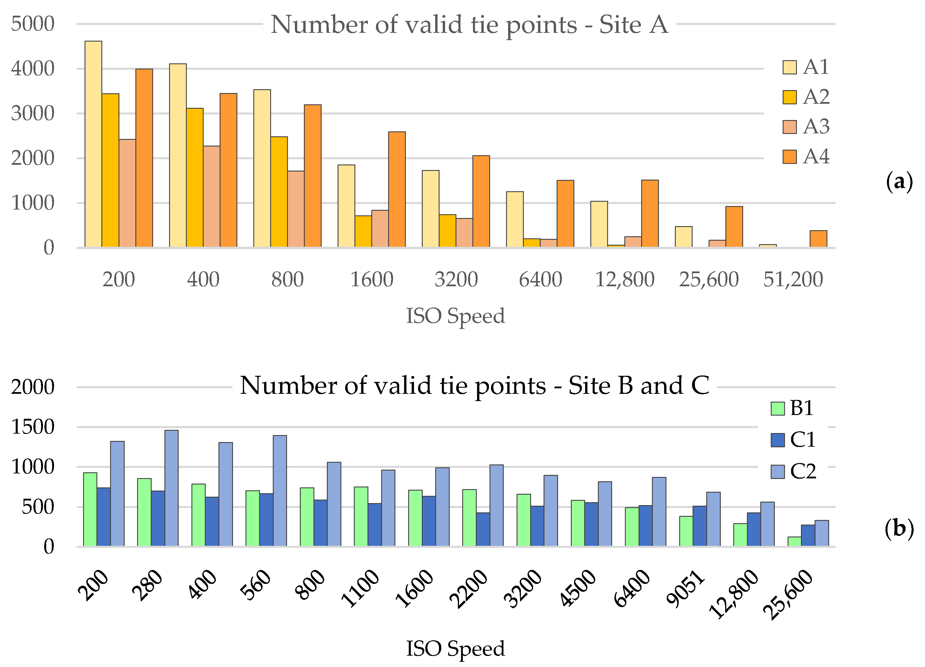
Table 1.
Nikon D810 specifications (D800 specifications indicated in parenthesis if different).
| Sensor | 36.3 MP FX | Native ISO | 64–12,800 (100–6400) |
| Sensor Size | 35.9 × 24 mm | Boost High ISO | 25,600–51,200 (12,800–25,600) |
| Resolution | 7360 × 4912 pixels |
Table 2.
Site specific image acquisition and block parameters.
| Site A | Site B | Site C | |
|---|---|---|---|
| Optics | Nikkor f/1.8 | Sigma f/2.8 | Nikkor f/1.8 |
| Focal length | 50 mm | 90 mm | 50 mm |
| Distance | 84 m | 245 m | 145 m |
| Base length | 26.7 m | 55.5 m | 39.4 m |
| GSD | 8.2 mm | 13.2 mm | 14.1 mm |
Table 3.
Summary of test conditions.
| Name | Date | Moon | Weather | Absolute EV | Distance (m) | Base Length (m) | Focal Length (mm) | GSD (mm) |
|---|---|---|---|---|---|---|---|---|
| A1 | 23/11/2018 (0:30 AM) | Full | Cloudy | −4 | 84 | 26.7 | 50 | 8.2 |
| A2 | 24/11/2018 (0:30 AM) | Full | Partly Cloudy | −4 | 84 | 26.7 | 50 | 8.2 |
| A3 | 19/02/2019 (1:30 AM) | Full | Clear | −4 | 84 | 26.7 | 50 | 8.2 |
| A4 | 20/02/2019 (1:30 AM) | Full | Partly Cloudy | −4 | 84 | 26.7 | 50 | 8.2 |
| B1 | 05/09/2020 (2:30 AM) | Full | Clear | −4 | 245 | 55.5 | 90 | 13.2 |
| C1 | 28/10/2020 (21:30 PM) | Full | Cloudy | −5 | 145 | 39.4 | 50 | 14.1 |
| C2 | 29/10/2020 (21:30 PM) | Full | Cloudy | −5 | 145 | 39.4 | 50 | 14.1 |
Table 4.
Summary of image acquisition and DSM reconstruction.
| Name | Stereo-Pairs | DSM (Total) | DSM (Valid) | DSM (Failed) | Relative EV (Number of Stereo-Pairs) | ||||
|---|---|---|---|---|---|---|---|---|---|
| −1.0 | −0.5 | 0.0 | +0.5 | +1.0 | |||||
| A1 | 77 | 308 | 252 | 56 | 32 | 0 | 42 | 0 | 3 |
| A2 | 77 | 308 | 152 | 156 | 32 | 0 | 42 | 0 | 3 |
| A3 | 81 | 324 | 226 | 98 | 32 | 0 | 42 | 0 | 7 |
| A4 | 81 | 324 | 288 | 36 | 32 | 0 | 42 | 0 | 7 |
| B1 | 117 | 468 | 463 | 5 | 21 | 15 | 27 | 21 | 33 |
| C1 | 120 | 480 | 480 | 0 | 21 | 15 | 28 | 21 | 35 |
| C2 | 119 | 476 | 476 | 0 | 21 | 15 | 28 | 20 | 35 |
| Total | 672 | 2688 | 2337 | 351 | 191 | 45 | 251 | 62 | 123 |
Table 5.
Aggregated (by site) average RMS differences using raw and Wallis-filtered images.
| Site | Raw (m) | Wallis (m) | Difference (%) |
|---|---|---|---|
| A | 0.044 | 0.044 | −0.7 |
| B | 0.048 | 0.049 | −3.4 |
| C | 0.047 | 0.048 | −2.6 |
Table 6.
Number of failed DSM reconstructions (Site A) based on image down-sampling ratio.
| 1 (Ultra High) | 2 (High) | 3 | 4 (Medium) | |
|---|---|---|---|---|
| A1 | 56 (18.2%) | 4 (1.3%) | 0 | 0 |
| A2 | 156 (50.6%) | 30 (9.7%) | 17 (5.5%) | 1 (0.3%) |
| A3 | 98 (30.2%) | 13 (4.0%) | 4 (1.2%) | 2 (0.6%) |
| A4 | 36 (11.1%) | 0 | 0 | 0 |
| TOTAL | 346 (27.4%) | 47 (3.7%) | 21 (1.7%) | 3 (0.2%) |
Table 7.
Coefficient of determination R2 of the fitted IQA–RMS model for the different sites. The best results are indicated in bold.
Table 7.
Coefficient of determination R2 of the fitted IQA–RMS model for the different sites. The best results are indicated in bold.
| PSNR | SSIM | BRISQUE | IlNiqe | MIQI | |
|---|---|---|---|---|---|
| Site A | 4.7% | 25.2% | 34.3% | 48.7% | 9.6% |
| Site B | 16.5% | 71.6% | 7.8% | 3.1% | 11.7% |
| Site C | 32.4% | 76.5% | 68.4% | 32.3% | 11.7% |
Table 8.
Coefficient of determination R2 of the fitted IQA–RMS model for the different acquisitions. The best results are indicated in bold.
Table 8.
Coefficient of determination R2 of the fitted IQA–RMS model for the different acquisitions. The best results are indicated in bold.
| PSNR | SSIM | BRISQUE | IlNiqe | MIQI | |
|---|---|---|---|---|---|
| A1 | 0.3% | 4.1% | 51.4% | 71.0% | 15.6% |
| A2 | 1.9% | 42.3% | 70.6% | 38.5% | 12.2% |
| A3 | 12.6% | 56.3% | 64.5% | 56.2% | 29.2% |
| A4 | 5.2% | 11.2% | 38.9% | 63.1% | 0.1% |
| B1 | 16.5% | 71.6% | 7.8% | 3.1% | 11.7% |
| C1 | 22.7% | 79.1% | 64.7% | 30.8% | 7.1% |
| C2 | 38.2% | 86.2% | 70.8% | 32.0% | 15.8% |
Table 9.
R2 of the robust fitted IQA–RMS model for the different sites. Values in brackets indicate differences compared to not robust fitted results.
Table 9.
R2 of the robust fitted IQA–RMS model for the different sites. Values in brackets indicate differences compared to not robust fitted results.
| PSNR | SSIM | BRISQUE | IlNiqe | MIQI | |
|---|---|---|---|---|---|
| Site A | 18.1% (+13.5%) | 37.9% (+12.8%) | 47.2% (+13.0%) | 62.2% (+13.5%) | 23.4–43.0% |
| Site B | 75.8% (+59.3%) | 80.3% (+8.7%) | 10.6% (+2.8%) | 0.0% (−3.1%) | N/A–18.8% |
| Site C | 78.2% (+45.8%) | 81.4% (+4.9%) | 80.4% (+12.0%) | 45.9% (+13.7%) | 32.1–56.4% |
Table 10.
R2 of the robust fitted IQA–RMS model for the different acquisitions. Values in brackets indicate differences compared to not robust fitted results.
Table 10.
R2 of the robust fitted IQA–RMS model for the different acquisitions. Values in brackets indicate differences compared to not robust fitted results.
| PSNR | SSIM | BRISQUE | IlNiqe | MIQI | |
|---|---|---|---|---|---|
| A1 | 35.9% (+35.6%) | 13.0% (+9.0%) | 56.2% (+4.8%) | 80.6% (+9.6%) | 27.2–94.7% |
| A2 | 27.4% (+25.4%) | 49.0% (+6.7%) | 78.3% (+7.6%) | 52.5% (+14.0%) | 32.5–67.2% |
| A3 | 72.4% (+59.8%) | 67.0% (+10.7%) | 73.0% (+8.5%) | 68.6% (+12.4%) | 53.9–74.7% |
| A4 | 13.8% (+8.7%) | 30.6% (+19.4%) | 57.1% (+18.2%) | 76.4% (+13.4%) | 0.1–57.6% |
| B1 | 75.8% (+59.3%) | 80.3% (+8.7%) | 10.6% (+2.8%) | 0.0% (−3.1%) | N/A–18.8% |
| C1 | 78.8% (+56.1%) | 82.0% (+2.9%) | 76.7% (+12.0%) | 39.7% (+8.8%) | 51.0–60.1% |
| C2 | 79.7% (+41.5%) | 91.4% (+5.2%) | 84.2% (+13.4%) | 48.1% (+16.1%) | 41.5–57.8% |
Publisher’s Note: MDPI stays neutral with regard to jurisdictional claims in published maps and institutional affiliations. |
© 2021 by the authors. Licensee MDPI, Basel, Switzerland. This article is an open access article distributed under the terms and conditions of the Creative Commons Attribution (CC BY) license (http://creativecommons.org/licenses/by/4.0/).
Share and Cite
MDPI and ACS Style
Roncella, R.; Bruno, N.; Diotri, F.; Thoeni, K.; Giacomini, A. Photogrammetric Digital Surface Model Reconstruction in Extreme Low-Light Environments. Remote Sens. 2021, 13, 1261. https://doi.org/10.3390/rs13071261
AMA Style
Roncella R, Bruno N, Diotri F, Thoeni K, Giacomini A. Photogrammetric Digital Surface Model Reconstruction in Extreme Low-Light Environments. Remote Sensing. 2021; 13(7):1261. https://doi.org/10.3390/rs13071261
Chicago/Turabian StyleRoncella, Riccardo, Nazarena Bruno, Fabrizio Diotri, Klaus Thoeni, and Anna Giacomini. 2021. "Photogrammetric Digital Surface Model Reconstruction in Extreme Low-Light Environments" Remote Sensing 13, no. 7: 1261. https://doi.org/10.3390/rs13071261
Note that from the first issue of 2016, this journal uses article numbers instead of page numbers. See further details here.