Article

Knowledge and Spatial Pyramid Distance-Based Gated Graph Attention Network for Remote Sensing Semantic Segmentation

School of Resources and Environmental Engineering, Wuhan University of Technology, Wuhan 430070, China
*
Author to whom correspondence should be addressed.
Remote Sens. 2021, 13(7), 1312; https://doi.org/10.3390/rs13071312
Submission received: 17 February 2021 / Revised: 24 March 2021 / Accepted: 26 March 2021 / Published: 30 March 2021
(This article belongs to the Special Issue Computer Vision and Deep Learning for Remote Sensing Applications)

Abstract

:
The pixel-based semantic segmentation methods take pixels as recognitions units, and are restricted by the limited range of receptive fields, so they cannot carry richer and higher-level semantics. These reduce the accuracy of remote sensing (RS) semantic segmentation to a certain extent. Comparing with the pixel-based methods, the graph neural networks (GNNs) usually use objects as input nodes, so they not only have relatively small computational complexity, but also can carry richer semantic information. However, the traditional GNNs are more rely on the context information of the individual samples and lack geographic prior knowledge that reflects the overall situation of the research area. Therefore, these methods may be disturbed by the confusion of “different objects with the same spectrum” or “violating the first law of geography” in some areas. To address the above problems, we propose a remote sensing semantic segmentation model called knowledge and spatial pyramid distance-based gated graph attention network (KSPGAT), which is based on prior knowledge, spatial pyramid distance and a graph attention network (GAT) with gating mechanism. The model first uses superpixels (geographical objects) to form the nodes of a graph neural network and then uses a novel spatial pyramid distance recognition algorithm to recognize the spatial relationships. Finally, based on the integration of feature similarity and the spatial relationships of geographic objects, a multi-source attention mechanism and gating mechanism are designed to control the process of node aggregation, as a result, the high-level semantics, spatial relationships and prior knowledge can be introduced into a remote sensing semantic segmentation network. The experimental results show that our model improves the overall accuracy by 4.43% compared with the U-Net Network, and 3.80% compared with the baseline GAT network.

Graphical Abstract

1. Introduction

Currently, the pixel-based methods [1,2,3,4,5] tend to take pixels as recognitions units to achieve remote sensing semantic segmentation, fuse the information of the area covered by the convolution kernel through the convolution operation. However, these methods cannot use high-level semantics, such as spatial relations and other information. Besides, the receptive fields in convolution are limited (generally 3 × 3) [6] and unevenly distributed [7], so it is hard to integrate context information of a larger area or obtain global information more evenly.
In response to the above problems, different scholars have carried out fruitful research [8,9]. Although the non-local method [8] can more effectively use the context information of the sample, it is computationally expensive and lack high-level semantics, such as spatial relations and other information.
With the development of graph neural networks, they have attracted increasing attention in GNN-based semantic segmentation [10,11,12]. Comparing with the pixel-based semantic segmentation methods, the current GNNs usually take objects as input nodes, in which computational complexity is relatively small. Besides, they are free from salt-and-pepper effects and can carry richer semantic information. However, the following two problems urgently need to be solved for them to be better applied in remote sensing recognition:
(1) Confusion of “different objects with the same spectrum”
The phenomenon of “different objects with the same spectrum” is a common problem in remote sensing analysis. To correctly identify the objects which are disturbed by this problem, it often requires knowing their surrounding objects. If considering only the similarity of the spectral features, such as the adjacency matrix based on similarity of nodes in graph attention network (GAT), the network will be vulnerable to this problem, thereby resulting in the misclassification of central node. The following figure shows two types of this problem: the flat_field and the town; the city_grass and the flat_field.
As shown in Figure 1, without the surrounding environment, the spectral of the town object A is similar to the flat_field object B, and the spectral of the city_grass object D is similar to that of the flat_field object C. Therefore, it is necessary to fuse the spatial relationships into the adjacency matrix. However, the spatial relationship derived from an individual sample often leads to the following problems.
(2) Confusion of spatial distance—“violating the first law of geography”
According to Tobler’s first law of geography, everything is related to everything else, but near things are more related to each other [13]. However, due to the limitation of the sample cutting the neighbors of some nodes in the sample may not be complete and accurate. If the spatial relationship is only considered in the individual sample, it will cause the distortion of the spatial relationships between the node and their neighbors, and may lead to the misclassification of the node. The following, Figure 2, shows two objects that are cut at the corners of samples.
According to the aggregation principle of GNNs, the neighbor nodes will their influence on the central node. When considering the spatial relationships, the weight of an individual object becomes smaller as the distance increases. The following, Figure 3, shows a central node and its neighbors.
As in the schematic diagram, O i is the central node, O j 1 , O k 2 , and O l 3 represent the neighbor node with a spatial distance of 1, 2, and 3, respectively. Then, the aggregation formula of the central node O i can be expressed as follows:
O i = O i + j N 1 α i j 1 O j 1 + k N 2 α i k 2 O k 2 + l N 3 α i l 3 O l 3 ,  
where N 1 , N 2 , N 3 represent the set of neighbour nodes with a spatial distance of 1, 2, and 3, respectively, and α is the aggregation weight.
The farther the distance from the central node is, the more the number of equidistant neighbor nodes there are, i.e., N 1 < N 2 < N 3 . If there are geographic objects with same category in the far distance, they may accumulate to cause a greater impact on the central node, even more than the nearby objects. This may lead to the problem of “violating the first law of geography”, and cause the misclassification of the central node.
Considering these, it is hard for the traditional GNNs to effectively solve the above two problems because they rely only on the context information of the individual sample. Therefore, it may require geographic prior knowledge based on the whole research area to solve them.
Therefore, the KSPGAT network, which is a remote sensing semantic segmentation model based on prior knowledge, spatial pyramid distance and GAT with gating mechanism is proposed. The KSPGAT network takes geographic objects as the unit of segmentation. Its computational complexity is relatively small, and it is free from salt-and-pepper effects. Additionally, it can carry richer and higher-level semantics, such as spatial relations and the category co-occurrence prior knowledge; thereby, it can better recognize the objects disturbed by the above two problems.
In summary, the main contributions of this paper are as follows:
(1) A novel spatial correlation recognition algorithm based on the spatial pyramid distance is proposed.
(2) A gating mechanism based on prior knowledge is proposed to realize the control of aggregation of neighbor nodes in graph neural network.
(3) A graph neural network model for remote sensing semantic segmentation is constructed, which effectively integrates the similarity of geographic objects, spatial relationships and global geographic prior knowledge.
The remainder of this paper is organized as follows: Section 2 discusses related work. A remote sensing semantic segmentation model based on prior knowledge, spatial pyramid distance and GAT with gating mechanism is presented in Section 3. The experiments are provided in Section 4. In addition, the analysis is presented in Section 5. The conclusion is provided in Section 6.

2. Related Work

2.1. Geographic Object-Based Image Analysis (GEOBIA)

Unlike pixels, which are usually the smallest unit of RS image analysis, image-objects are defined by Hay et al. [14] as basic entities, located within an image that are perceptually generated from H-res pixel groups. As geographic objects can provide rich spatial relationships information than pixels, the OBIA methods are making considerable progress.
The OBIA methods usually use segmentation algorithm to obtain the objects first and then use the objects for subsequent image analysis. Currently, the OBIA methods are widely applied in multi-scale research [15,16], change detection [17] and landslide detection [18]. To better understand ecological patterns, it is also expanded to the species-level mapping of vegetation [19]. Other research, like References [20,21], presented a comparative evaluation of the pixel-based method and the object-based; especially, Reference [21] compared the pixel-based support vector machine (SVM) classification and decision-tree-oriented geographic object-based image analysis (GEOBIA) classification, which indicated that the GEOBIA classification provided the highest accuracy. Besides, work, like Reference [22], discussed the idea and method of geographic ontology modeling based on object-oriented remote sensing technology in detail.
On this basis, the GEOBIA methods based on neural networks have attracted an increasing attention. For example, the research in Reference [23] proposed a novel land use classification method for high-resolution remote sensing images, and the method is based on a parallel spectral-spatial convolutional neural network (CNN) and object-oriented remote sensing technology. On the basis of geographic object-based image analysis, other works, like Reference [24], presented an artificial neural network (ANN) which integrated with particle swarm optimization (PSO) to enhance the learning process.
Based on these research, our work attempts to combine the GEOBIA and neural networks, and explores further in this direction.

2.2. Remote Sensing with GNN

As an important branch of the deep learning family, the strategy based on graph neural networks [25,26] have grown more and more popular, which achieves the state-of-the-art performance in both graph feature extraction and classification. Among them, graph convolutional network (GCN) [27] plays an important role. Furthermore, Reference [28] proposes a novel neural network called graph attention networks (GATs) which can attend over their neighborhoods’ features and specify different weights to different nodes in a neighborhood, without requiring any kind of costly matrix operation (such as inversion) or depending on knowing the graph structure upfront. Inspired by these, applying deep neural networks to graph structured data has recently been of interest to the vision community. For example, approaches, such as References [29,30], tried to generalize convolution layers to the graphs. Other works, like References [31,32], attempted to learn knowledge graphs and use graphs for visual reasoning.
However, the current GNN networks directly stacking more layers will bring the problem of over-smoothing, which drives the output of GCN towards a space that contains limited distinguished information among nodes, leading to a poor expressivity. To solve this problem, many researchers have recently conducted beneficial explorations. Some of them try to use used random-walk method [33] or restrict the neighborhood expansion size [34,35] to solve this issue. There are also some studies alleviate this issue by deleting the edges in the graph [36] or incorporate multi-hop neighboring context into attention computation [37].
Apart from these, combining a prior knowledge base with GNN models for vision tasks also becomes popular. Reference [38] used the knowledge graph to perform zero-shot classification. References [39,40,41] used the common-sense or structured prior knowledge to improve the performance of deep models. Other works, like References [42,43,44], tried to use graph embedding to learn some prior knowledge or relationships between label.
In the research of remote sensing image analysis, as hyperspectral images usually have large homogeneous regions, some research started to use graph neural networks (GNNs) to achieve remote sensing images analysis [45,46,47,48]. For example, Reference [45] investigated the use of graph convolutional networks (GCNs) in order to characterize spatial arrangement features for land use classification and [46] proposed a novel deep learning-based MLRSSC framework by combining graph neural network (GNN) and convolutional neural network (CNN) to mine the spatio-topological relationships of the scene graph. To further improve the detection accuracy, Reference [49] proposed a novel anomaly detection method based on texture feature extraction and a graph dictionary-based low rank decomposition (LRD).
Currently, some other scholars have also started to integrate the geographic prior knowledge into remote sensing analysis. Works, like Reference [50], presented a spatial location constraint for hyperspectral image classification, which is exploited to incorporate the prior knowledge of the location information of training pixels. Similarly, to further improve the recognition performance, Reference [51] proposed a simplified graph-based visual saliency model for airport detection in panchromatic remote sensing images, which introduced the concept of near parallelity for the first time and treated it as prior knowledge.
In summary, in remote sensing analysis research, the pixel-based methods are computationally expensive and cannot contain object-based spatial relationships and geographic prior knowledge. Most current GNN methods can carry richer semantic and their computational complexities are relatively small, but they rarely consider geographic prior knowledge. Therefore, to better introduce the prior knowledge into remote sensing analysis, it still needs further exploration.

3. Methodology

In this chapter, the overall structure of the KSPGAT network is introduced first in Section 3.1. To solve the problem of “different objects with the same spectrum”, a novel spatial pyramid distance algorithm is presented in Section 3.3. Further research shows that only rely on the spatial relationships between geographic objects cannot effectively solve the problem of “violating the first law of geography”. For this reason, a gating mechanism which embeds geographic prior knowledge into the GAT model is then introduced in Section 3.4 and Section 3.5, and it can solve the two problems to some extent. Finally, considering the problem of over-smoothing in graph neural networks, we design the network depth into two layers, and incorporate the effect of co-occurrence knowledge in the loss function in Section 3.6.

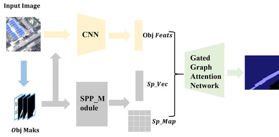
3.1. Network Structure

The KSPGAT network is designed as the encoder-decoder structure and consists of four modules, of which the superpixel clustering module, feature extraction module, and spatial correlation recognition algorithm together constitute the encoder, the knowledge-based gating mechanism is the decoder. The details are shown as follows:
As shown in Figure 4, in our network, a super-pixel clustering module and a feature extraction module are proposed to obtain the object features from the input remote sensing image first. Then, a spatial pyramid distance recognition algorithm is provided to recognize the spatial relationship between objects. Finally, on the basis of fusing the feature similarity and spatial relationship, a multi-source attention mechanism and a gating mechanism are presented to aggregate neighbor nodes more accurately. Specifically, the network contains the following modules.

3.1.1. Superpixel Clustering Module

The region merging segmentation method proposed in References [52,53,54] is used to perform superpixel clustering of remote sensing images, so each sample can obtain several superpixel blocks. Then, these superpixel blocks are used to provide masks for feature extraction module and spatial correlation recognition algorithm.

3.1.2. Feature Extraction Module

The feature extraction module of the network takes the remote sensing image and the object mask as input to obtain object features. First, the remote sensing image is extracted through a convolutional neural network (CNN) to obtain the global feature. Then, the mask is used to obtain the feature of each object. Finally, the node of the graph neural network is generated through the object feature.

3.1.3. Spatial Correlation Recognition Algorithm Based on Spatial Pyramid Distance and Multi-Source Attention Mechanism

In this module, we propose a novel spatial correlation recognition algorithm. First, we design the location coding method based on pyramid pooling to obtain the location coding vector of each object, and then we use the vector to identify the spatial distance between objects, which is simple and efficient enough to generate the spatial correlation between nodes. Finally, the similarity of features and the spatial correlation between nodes are combined to design and implement the multi-source attention mechanism.

3.1.4. Gating Mechanism Based on Prior Knowledge of Category Co-Occurrence

The gating mechanism uses category co-occurrence knowledge to train control gates corresponding to different spatial pyramid distances (spatial relations). It realizes the aggregation method that integrates knowledge, spatial relations and node similarity, thereby improving the classification accuracy of the central node.
The following subsections will expand on each module of the network.

3.2. Superpixel Clustering Module and Feature Extraction Module

First, the region merging segmentation method proposed in References [52,53,54] is used to perform super-pixel clustering of remote sensing images so each sample can obtain several superpixel blocks. Each superpixel block is a geographical object with geographic semantics, which can be used as a H 4 × W 4   mask. Then, the feature extraction module is adopted to extract object features with this mask. The following, Figure 5, shows the structure of feature extraction module:
As shown in Figure 5, the feature extraction module first takes the remote sensing image (W × H × 3) and the object masks (N × W/4 × H/4) as input, where N is the number of objects. Then, the remote sensing image is passed through a CNN to obtain the global feature, which is multiplied by the mask to obtain the masked object features (N × W/4 × H/4 × C), where C is the hidden dimension. The masked object features are sent to two branches, respectively, and then concatenated to obtain the final feature F e a t , which has dimension N × (C + 49), and is used as the initial node feature h of the graph network.
The calculation formula of this module is as follows:
h = G ( ( F ( x ) . Mask ) ) ,  
where x is the input image, F(.) is the global feature extraction function, which consists of two convolutional layers and pooling layers, Mask is the object mask, and G(.) is the feature extraction function, which consists of two branches, one a global average pooling (GAP) layer, and the other a max pooling layer with convolutional layer.

3.3. The Spatial Correlation between Objects: The Spatial Pyramid Distance

In this section, we introduce a novel location encoding method based on pyramid pooling, and on this basis, we propose the spatial pyramid distance to represent the spatial correlation between objects. The details are as follows.

3.3.1. The Location Encoding Method Based on Pyramid Pooling

Pyramid pooling is used to encode the two-dimensional position information of the object mask. The object mask is passed through 3-level pyramid average pooling (28 × 28, 14 × 14, 7 × 7) to obtain multiscale spatial location features. We use the area ratio of the mask in the pooling kernel to calculate the pooled value, which includes the semantic of object’s area. The formula of average pooling is as follows:
c p q k = i = p p + k j = q q + k M a s k i j k × k ,  
where k is the size of pooling kernel, M a s k is the object mask, p is the start index in row, q is the start index in column, and c p q is the value after pooling.
Then, the location features are encoded into a one-dimensional vector by quadtree-encoding. The vector e can be defined as follows:
e k = { c p q k } ,  
e = c o n c a t ( e k , ) ,  
where k represents the size of pooling kernel, and k 28 , 14 , 7 . {.} represents the quadtree-encoding, c o n c a t ( . ) means vector concatenation.
In this way, the approximate location of each object can be obtained, and the value of each grid represents the semantic of object’s area. The following, Figure 6, shows two object masks’ position vector after spatial pyramid pooling.
After the pooling of three scales, there exists a significant difference between the encoding vectors of the two objects with long distance, which is conducive to the subsequent spatial distance recognition.

3.3.2. Spatial Pyramid Distance

On the basis of the above location encoding method, to describe the spatial relationships between nodes, we define the spatial pyramid distance to discretely represent them. According to the number of other interval objects between node i and j, interval_number = 0 means that the two nodes are directly adjacent, interval_number = 1 means that there is only one object between them, and interval_number 2 means that there are multiple objects between them. Based on this, the spatial pyramid distance s p _ m a p i j between node i and j is defined as Table 1:
Therefore, the three different values of s p _ m a p i j represent spatial adjacency, spatial separation (near), and spatial separation (far), respectively.

3.3.3. The Spatial Correlation Recognition Algorithm Based on Spatial Pyramid Distance

Based on the location encoding method and spatial pyramid distance, we design a spatial correlation recognition algorithm. The algorithm is used to describe the spatial distance between geographical objects discretely according to three different values, where 1 represents spatial adjacency, 2 represents spatial separation (near) and 3 represents spatial separation (far).
The algorithm is denoted by the Algorithm 1:
Algorithm 1 For recognizing the spatial pyramid distance
Input: mask of object i m a s k i , mask of object j m a s k j
Output: distance feature vector   s p _ v e c i j , spatial pyramid distance s p _ m a p i j
   1  Begin
   2  For t 1 to 3 step 1; do
   3   k 56 2 t ; // calculate the pooling size k
   4   e k i a v g p o o l i n g k ( m a s k i ) ; // encode the position vector of m a s k i with pooling size k
   5   e k j a v g p o o l i n g k ( m a s k j ) ; // encode the position vector of m a s k j with pooling size k
   6  End For
   7   c o n c a t e n a t e all e k i to obtain the multiscale location features e i of m a s k i ;
   8   c o n c a t e n a t e all e k j to obtain the multiscale location features e j of m a s k j ;
   9   v i j e i e j ; // subtract the position encoding vectors of m a s k i and m a s k j
   10   s p _ v e c i j f c 1 ( v i j ) ;
   11   s p _ m a p i j f c 2 ( s p _ v e c i j ) ;
   12  Return s p _ v e c i j , s p _ m a p i j ;
   13  End
Then, we design a network to accomplish the algorithm, the structure of the network is as Figure 7:
The network takes the mask of each pair of objects as input, which can be expressed as ( N × N ) × H 4 × W 4 × 2 . Then, the location encoding method based on pyramid pooling is used to obtain the spatial location vectors at different scales. To fuse these features, they are, respectively, coded into one-dimensional vectors and obtain the multiscale location features Position   Features . Then, two Position   Features subtract to obtain the distance features and passes through a Multi-layer Perceptron (MLP) layer to obtain the distance feature vector   Sp _ Vec between each pair of objects, and finally passes through another MLP layer to obtain the spatial pyramid distance Sp _ Map .
In our dataset, the overall accuracy of the algorithm reaches 83.6%, which can basically describe the spatial distance between objects. Therefore, it can provide a favorable basis for subsequent node classification.
Compared with the spatial relationship analysis method in GIS or other neural networks, our method contains the following advantages:
(a) As it uses the area ratio of the mask in the pooling kernel to calculate the pooled value, it contains richer semantics of object’s area;
(b) Unlike the method based on the centroid distance between objects, it is easy to be implemented;
(c) Compared with other neural networks based on object detection, it does not require complex computations, which reduces the network pressure and therefore improves the generalization ability.
In summary, this algorithm can efficiently construct the adjacency matrix between nodes and quickly provide reliable input for the graph neural network. Based on the algorithm, the KSPGAT network then combines the spatial relationship and the similarity of features to design and implement the following multi-source attention mechanism.

3.4. Multi-source Attention Mechanism Based on Similarity of Spectral Features and Spatial Relationships of Geographic Objects

In this section, we first analyze the problem of the attention mechanism in the baseline GAT, and then we propose our multi-source attention mechanism.

3.4.1. Attention Mechanism in the Baseline GAT

The attention mechanism in the baseline GAT only considers the similarity of the spectral features between nodes. Assuming that the original node feature is h, first the node feature is multiplied by a weight W h to project the feature into a new space. Then, to consider the feature similarity between nodes i and j , the transformed features of two nodes are concatenated, and the feature similarity is calculated through a weight a . Finally, the correlation between the two nodes, which is defined as α i j , can be obtained through a softmax function. The specific calculation formula is as follows:
e i j = a ( W h . h i   | | W h . h j ) ,  
α i j = s . s o f t m a x ( e i j ) ,  
where W h is a learnable weight to project the spectral features of nodes, || represents vector concatenation, softmax is the normalized function by row, and s is the scaling factor to prevent the weight of neighbours from being too small.
As this mechanism is more rely on spectral similarity to aggregate neighbor nodes, it cannot solve the problem of “different objects with the same spectrum”. Therefore, it is necessary to integrate spatial relationships into the attention mechanism to improve it. The improved algorithm is as follows:

3.4.2. Multi-Source Attention Mechanism Based on Geographic Object Feature Similarity and Pyramid Distance

In the multi-source attention mechanism, to solve the problem of “different objects with the same spectrum”, we consider not only the similarity of the spectral features between the geographic objects, but also the spatial pyramid distance between them. We multiply the distance feature S p _ V e c i j of nodes i and j by a weight W s to project the distance feature into the same space as spectral features and then concatenate it with the transformed spectral features of nodes i and j . Therefore, the algorithm for calculating attention becomes as follows:
e i j = a ( W h . h i   | | W h . h j   | | W s . s p _ v e c i j ) ,  
α i j = s . s o f t m a x ( e i j ) ,  
where W h is a learnable weight to project the spectral features of nodes, W s is a learnable weight to project the distance features, || represents vector concatenation, softmax is the normalized function by row, and s is the scaling factor to prevent the weight of neighbours from being too small.
However, due to the problem of “violating the first law of geography” discussed in Section 1, the aggregations of neighbor nodes are still under great limitations even considering the spatial relationship. At this time, the following gating mechanism based on category co-occurrence knowledge is represented to control the aggregation of neighbor nodes more accurately.

3.5. Knowledge-Based Gating Mechanism

To overcome the problem of “violating the first law of geography” caused by the distortion of the spatial relationship at the corner of samples in some area, we first summary the co-occurrence probability between different categories from the whole dataset and then design a gated graph attention network which uses the co-occurrence probability to expand the receptive field of the object from the specific sample to the whole research area. This corrects some distortion problems of spatial relationship, thereby improving the accuracy of remote sensing semantic segmentation. Furthermore, through the gating mechanism, the neighbor nodes are filtered based on the prior knowledge; thereby, the mechanism can avoid the problem of over-smoothing to a certain extent.

3.5.1. Category Co-Occurrence Knowledge in the Sample Set

Category co-occurrence means the probability of two categories appearing in a scene at the same time. As shown in Figure 8 below, M is the category co-occurrence matrix, which represents co-occurrence between each category. The size of M is C × C , where C   is the number of categories. M i j represents the proportion of samples S i j with both categories i and j among all samples S i with category i , i.e., M i j = S i j / S i . The figure below shows the category co-occurrence probability matrix, which means the probability of two categories appearing in a scene at the same time.
As discussed in Section 1, due to the limitation of the sample cutting in some areas, the neighbors of some nodes in the sample may not be complete and accurate, which may cause the distortion of the spatial relationship between the nodes and their neighbors. The co-occurrence relationship is a more universal relationship obtained according to the co-occurrence probability in the dataset which describe the general geographic prior knowledge of the research area. Therefore, the weight of the nodes can be strengthened or weakened according to the co-occurrence probability. This can correct some distortion problems of spatial relationship, and alleviate the problem of “violating the first law of geography”, thus make the aggregation of neighbor nodes more accurate.
Based on the above-mentioned category co-occurrence knowledge, we then design the following gated graph attention network and use the category co-occurrence GT to train the control gate.

3.5.2. Gated Graph Attention Network Based on Category Co-Occurrence Prior Knowledge

In this section, we introduce our novel gated graph attention network. In the network, we divide all neighbor nodes into k groups according to their spatial correlation with the central node. For each group, we design a gating mechanism. During the training phase, the co-occurrence knowledge of two categories are used to control the aggregation of neighbor nodes, thereby correcting the problems of “violating the first law of geography”. Furthermore, through the gating mechanism, the neighbor nodes are filtered based on the prior knowledge; thereby, the mechanism can avoid the problem of over-smoothing to a certain extent.
(1) Structure
Our gated graph attention network combines the multi-source attention mechanism, and is designed with a gating mechanism that integrates category co-occurrence knowledge to control the aggregation of neighbor nodes more accurate. Figure 9 below shows the structure of a head of the gated graph attention network.
As the major part of the KSPGAT network, for a central node i , the gated graph attention network takes its node feature h i , the node feature h j of its neighbor node j ( j i ), their distance vector Sp _ Vec i j and spatial pyramid distance Sp _ Map i j as the input. Then, the multi-source attention mechanism is combined and the gating mechanism is designed to aggregate the features of neighbor nodes. During the training phase, the prior knowledge of category co-occurrence is integrated into the gating mechanism by using category co-occurrence ground truth (GT) to supervise and train the control gates.
To better represent the co-occurrence relationship between nodes, we design the co-occurrence knowledge according to the probability P i j and P j i in the category co-occurrence matrix; if max { P i j , P j i } 0.5 , it can then consider that category i and category j have a co-occurrence relationship. At this time, the GT of the co-occurrence control gate is set to 1, which indicates that the gate is opened; otherwise, there is no co-occurrence relationship, and the GT is marked as 0 to indicate that the gate is closed.
(2) Aggregation with multi-group
Based on K (K = 3) spatial distances which are adjacent, separated (near), and separated (far), respectively, we divide all neighbor nodes into k groups. Therefore, K kinds of GAT heads are designed to aggregate neighbor nodes of different spatial relationships. For the GAT head of each spatial relationship, a gate which combines the category co-occurrence knowledge is designed to control the process of neighbor nodes aggregation. The following, Figure 10, shows the aggregation of the network.
As shown in Figure 10, network divides all nodes into k groups according to their spatial correlation with the central node to form a new GAT head with a gating mechanism, called gate_head.
The following, Figure 11, shows the flow chart of aggregation.
As shown in Figure 11, during node aggregation, the node features h, the distance vector Sp _ Vec and the spatial pyramid distance Sp _ Map are input into the gated graph attention network to generate the new node features h . N is the number of the nodes, and K is 3, which represents three kind of spatial distances. N k represents the number of the neighbor nodes with a spatial distance k.
For each central node i and one of its neighbour nodes j ( j i ), the spatial relationship between them is k , the aggregation of node i is as follows:
(a) First, h e a d i j k which can aggregate the information of node j to the central node i is calculated with h i , h j , s p _ v e c i j , s p _ m a p i j .
(b) Then, g a t e i j k is calculated with h i , h j , s p _ v e c i j , s p _ m a p i j . If nodes   i and j have a co-occurrence relationship, the g a t e i j k will be opened; otherwise, it will be closed.
(c) Finally, the new node features h i of the central node i is calculated with h e a d i j k and g a t e i j k of all neighbor nodes.
In summary, the control gate is calculated from the node feature, the embedded distance feature and the spatial pyramid distance. The specific formula is as follows:
h e a d i j k = α i j k W _ H h k . h j ,  
g a t e i j k = { σ ( a [ W _ G h k . h i   | | W _ G h k . h j   | | W _ G s k . s p _ v e c i j ] ) ,     s p _ m a p i j = k 0 ,     e l s e ,  
h i = W h . h i + j N i , j i k K g a t e i j k h e a d i j k ,  
where W _ G h k and W _ G s k are learnable weights in the gate that controls the k t h GAT head, N i represents all neighbour nodes of node i , W _ H h k   is a learnable weight in the k t h GAT head, and α i j k is the attention weight calculated by the multi-source attention mechanism in the k t h GAT head. K = 3 represents three spatial pyramid distances, and k = 1, 2, 3 indicates the spatial pyramid distance of 1, 2, and 3, respectively.
(3) Discussion
Different from the traditional attention aggregation mechanism, the KSPGAT network adopts multi-group aggregation mechanism with spatial relation. The gate _ h e a d divides all neighbor nodes into k groups according to their spatial correlation with the central node, and uses gates that integrate category co-occurrence knowledge to control the aggregation of neighbor nodes. Comparing with the traditional attention mechanism, the multi-group aggregation mechanism has the following advantages:
(a) Each group only contains the neighbor nodes that have the same spatial correlation with the central node. The neighbor nodes of each group have certain commonalities, and the head does not have parameter redundancy, which can reduce the training pressure;
(b) The gate controlled the process of aggregation neighbor nodes by integrating prior knowledge, and the controllability of the network and the interpretability of the results are improved.
(c) Through the gating mechanism, the neighbor nodes are filtered based on the prior knowledge; thereby, the mechanism can avoid the problem of over-smoothing to a certain extent.

3.6. Network Depth (Number of Aggregation) and Loss Function

In this section, we focus on the analysis of network depth and loss function in the KSPGAT network.

3.6.1. Depth of KSPGAT Network

Similar to the baseline GAT network, our KSPGAT network aggregates twice in total: In the first aggregation we adopt the same multi-head structure as the baseline GAT network. Specifically, use P (in our experiment P = 2) independent g a t e _ h e a d 1 p with gating mechanism to process the input node features h and then concatenate their output features together as the input feature h 1 of the second aggregation. In the second aggregation, only an independent g a t e _ h e a d 2 with gating mechanism is used to process the new input feature h 1 to obtain the output feature h 2 , and, finally, a softmax nonlinear function is used to obtain the classification probability o. The formula is as follows:
h 1 = g a t e _ h e a d 1 P ( h )   | | g a t e h e a d 1 P 1 ( h )   | | | | g a t e _ h e a d 1 1 ( h ) ,  
h 2 = g a t e _ h e a d 2 ( h 1 ) ,  
o = s o f t m a x ( h 2 ) ,  
where h is the original node feature, and P is the number of heads in the multihead structure. h 1 is the output feature of the first aggregation and also the input feature of the second aggregation, h 2 is the output of the second aggregation, and o is final classification probability.

3.6.2. Co-Occurrence Knowledge Embedding Loss

To implicitly embed the co-occurrence knowledge into the control gate, we added a co-occurrence knowledge embedding loss in our network in addition to the node classification loss. The co-occurrence knowledge embedding loss adjusts the network parameters by calculating the mean square error between the value of the co-occurrence knowledge gate and co-occurrence knowledge GT between nodes. The specific calculation formula of the co-occurrence knowledge embedding loss l o s s g a t e and the node classification Loss l o s s c l s is as follows:
l o s s g a t e =   1 K 1 N × N k = 1 K n = 1 N × N ( y ^ n k y n k ) 2 ,  
l o s s c l s = 1 N i N y i log ( y ^ i ) .
Furthermore, to balance the node classification loss and the co-occurrence knowledge embedding loss, we introduce a balance factor λ. Generally, λ is the maximum ratio of the two loss thresholds. In the experiment, we set λ = 10. Therefore, the total loss of the network is calculated as follows:
l o s s = l o s s c l s + λ l o s s g a t e .

4. Experiment

In this chapter, the introduction of research areas and samples is presented in Section 4.1 first. Then, we show the parameters of the networks which are involved in our experiment in Section 4.2. The overall accuracy comparison is conducted in Section 4.3. Finally, the training process and loss curve are shown in Section 4.4.

4.1. Introduction of Research Areas and Samples

This study involves Wenchuan County, Sichuan Province, and the surrounding areas. The latitude ranges from 30°45′ to 31°43′ and the longitude ranges from 102°51′ to 103°44′. We selected a total of 1680 patches from the research area. To make the number of samples in the validation set and training set sufficient and the results reasonable, we randomly assigned 1280 samples as the training set and the other 400 samples as the validation set. Each sample includes a 224 × 224 remote sensing image, a manually classified GT image of the same size, and an object mask obtained using the open source algorithms [52,53,54].

4.2. Network Parameters

The networks that are involved in the experiment include a U-Net network, a baseline GAT network, a multi-source GAT network and a KSPGAT network incorporating prior knowledge and spatial pyramid distance.
According to the previous experiment, when we train the U-Net network, the feature dimension in the bottom layer is set to 512, the batch_size is set to 32, the learning rate is set to 3e−4, and the training epochs is 250; The hidden dimensions of the baseline GAT network, multi-source GAT network and KSPGAT network are all 128, and are all aggregated twice. The baseline-based GAT network and the multi-source GAT network use 4 GAT heads for the first aggregation, and a single GAT head for the second aggregation; the KSPGAT network uses 2 gate _ h e a d with a gating mechanism in the first aggregation, and a single gate _ h e a d in the second aggregation. The batch_size of the three graph neural networks are all 1, the learning rates are all 1e−3, and the training epochs are all 600.

4.3. Overall Accuracy Comparison

To compare with the results of U-Net network, we convert the results of the three graph neural networks from objects to pixels. The classification results of the four networks on the validation set are as follows: Table 2, Table 3, Table 4 and Table 5 are pixel-based classification confusion matrices of the U-Net network, baseline GAT network, multi-source GAT network, and KSPGAT network, respectively.
Additionally, we further compare the four networks in other classification metrics, and the results are as Table 6.
It can be seen that the KSPGAT network also has a significant improvement in Accuracy, Mean Intersection over Union (MIOU), Kappa, and F1-Score compared to the other three networks.
By comparing the pixel-based classification results of the four networks, it can be seen that the classification results of the baseline GAT network and the U-Net network are similar. The overall accuracy of the U-Net network is 86.7%, and the baseline GAT network is 87.3%. Compared with the baseline GAT network, the multi-source GAT network increases its overall accuracy by 1.3%, reaching 88.6%. The most significant improvement has been made in the KSPGAT network, in which overall accuracy has been increased by 3.8% compared with the baseline GAT network, reaching 91.1%.
Further analysis shows that the classification accuracy of the baseline GAT network in the categories of village, path and forest is significantly higher than that of the U-Net network. However, these two networks have the following problems:
(1) The accuracy is low in the categories of city_forest and city_grass, which are prone to be confused with forest and grass;
(2) The accuracies of categories with a small number of samples are relatively low;
The following, Table 7, shows the accuracy comparison of the four networks in some categories.
From the above comparison, it can be seen that the classification accuracy of the U-Net network and the baseline GAT network on the city_grass and the city_forest is relatively low. Among them, the classification accuracies of the U-Net network in city_grass and city_forest are 28.7% and 25.1%, respectively. The classification accuracies of the baseline GAT network in city_grass and city_forest are 66.9% and 60.8%, respectively.
The multi-source GAT network has a slight improvement compared with the previous two networks, but the classification accuracies of city-grass and city-forest are still low, only 34.4% and 73.6%, respectively.
Compared with the baseline GAT network, the KSPGAT network, which integrates spatial pyramid distance and co-occurrence prior knowledge, has improved the classification accuracy of city_grass from 25.1% to 61.9%, and the classification accuracy of city_forest has increased from 60.8% to 85.7%.
After comparative analysis, it can be seen that the KSPGAT network with obvious advantages can greatly improve the classification accuracy of city-grass and city-forest by incorporating the spatial pyramid distance and co-occurrence prior knowledge.
To verify the stability of our KSPGAT network, we randomly allocate the total samples to the training and validation sets in the same proportions as the previous experiments, and performed 10 independent Monte Carlo runs. We compared the Accuracy, mIOU, Kappa, and F1-Score of the 10 experiments, where the trend is shown in Figure 12:
In the 10 experiments, the mean values of the Accuracy, mIOU, Kappa, and F1-Score were 0.9095, 0.8449, 0.9151, and 0.9138, respectively, and the standard deviations were 0.00259, 0.00287, 0.00290, and 0.00169, respectively, which proved the stability and reliability of the experimental results.
Besides, to compare the performance and system resource requirements of the four networks, we also conducted a benchmark test. With the hardware environment of RTX 3080 GPU, we used the same validation set to test Params, which means the model size; Mem, which means the training GPU memory consumption; FLOPs, which means the calculation amount; and Inf time, which means the inference speed of model. We conducted the benchmark test in this environment for 10 times and took the average results as the final test results. The benchmark test results are shown as Table 8.
By comparing the benchmark test result of each model, we can see that our KSPGAT model has obvious advantages in model size, resource occupation, calculation amount, and inference speed.
Further, to check the value of our method, we used another remote sensing semantic segmentation dataset, called Gaofen Image Dataset (GID) [55], for experimental comparison. The dataset contains 10 pixel-level annotated GF-2 images, which has two more categories than our previous dataset and is made up of 15 categories: paddy field, irrigated land, dry cropland, garden land, arbor forest, shrub land, natural meadow, artificial meadow, industrial land, urban residential, rural residential, traffic land, river, lake, and pond. Since the 10 images in the GID dataset come from different regions and cover a geographic area of 506 km2, to make a fair comparison with our previous experiment, we cut 1800 samples with a size of 224 × 224 to compose the new dataset in which size is similar with our previous dataset, and we allocated the training set and the validation set in a ratio of 7:3 according to the principle of random allocation, which is consistent with our previous experiment. Therefore, we obtained 1260 samples as training data and the remaining 540 samples as validation data. Then, we recalculated the category co-occurrence probability in the new dataset. Finally, we trained the four models on the training set with the same hyperparameters (batch size, learning rate, and training epochs) as the previous experiments and verified on the validation set. The results are shown in the following, Table 9.
It can be seen that our KSPGAT model improves the overall accuracy by 3.1% compared with the baseline GAT network and 4.5% with the U-Net network. The results mean that in different regions and different seasons, using different satellite data with larger categories, the effects of our model are stable and reliable. And this illustrates the value of our model.

4.4. Training Process and Loss Curve

All four networks use Adam optimizer for training, and their loss curves on the validation set are as shown in Figure 13:
As shown in Figure 13, the x-axis represents the number of network epochs, and the y-axis represents the loss during network training. The loss curve shows the convergence trend of the network. As the number of epochs increases, in the early training period, the curve oscillates and decreases, and it stabilizes towards the later stage. We train the four networks for 600 epochs, but the U-Net network is overfitting after 250 epochs. To ensure complete network convergence without overfitting, we choose 250 as the training epoch for the U-Net network, and 600 for the baseline GAT network, the multi-source GAT network, and the KSPGAT network.

5. Results

According to the two problems discussed in Section 1, we analyze the recognition capabilities of three object-based networks in the two problems separately, in which the analysis of the problem “different objects with the same spectrum” is conducted in Section 5.3, the analysis of the problem “violating the first law of geography” is shown in Section 5.4. Finally, the discussion of the three networks are represented in Section 5.5.
To show the advantages of the KSPGAT network, we analyze the classification effects of the four networks in some typical samples, as shown in Figure 14:
Comparing the classification results of three object-based models, it can be found that sample I and sample II can be classified completely correct in all three networks. Sample III and sample IV cannot be correct classified in the baseline GAT network, but can be classified completely correct in both the multi-source GAT network and the KSPGAT network. Sample V and VI can only be classified completely correct in the KSPGAT network.
Further comparing, the classification effect of the three object-based graph neural networks is significantly better than that of the U-Net network. The U-Net network accomplishes segmentation pixel by pixel, which leads to the problem of salt-and-pepper phenomena. While three graph neural networks accomplish segmentation based on superpixel blocks, and are free from salt-and-pepper effects.
To check the value of our method in other dataset, we show the classification results of four models in GID [55]. The classification results are shown in Figure 15.
As shown in Figure 15, our KSPGAT model also outperforms several other models in the GID dataset, which proves the value of our method in other different areas.
To analyze the advantages of the KSPGAT network during node aggregation, according to the two problems discussed in Section 1, we divide the several samples in Figure 13 to two groups, wherein one is disturbed by the problem of “different objects with the same spectrum”, and the other is interfered by the problem of “violating the first law of geography”.

5.1. The Problem of “Different Objects with the Same Spectrum” in Sample III, IV

The phenomenon of “different objects with the same spectrum” is a common problem. To correctly identify the objects which are disturbed by this problem, it often requires knowing the surrounding objects. The following, Figure 16, shows the samples with this problem:
As seen in Figure 16, the spectrums of town object A and flat_field object B in (a) are similar; the spectrums of flat_field object C and city_grass object D in (c) are similar. Therefore, they all have the problem of “different objects with the same spectrum”. Without the information of the surrounding environment, it is hard to identify their actual categories.

5.2. The Problem of “Violating the First Law of Geography” in Sample V and VI

Due to the limitation of the sample cutting in some areas, the neighbors of some nodes in the sample may not be complete and accurate, which will cause the distortion of the spatial relationships. The following, Figure 17, shows the samples with this problem.
As seen, the forest object A in Figure 17a and the city_forest object B in Figure 17c are cut at the corner of the sample. As their spatial relationships with neighbors are distorted, they may be interfered by the problem of “violating the first law of geography”.
In these two group of samples, we choose the flat _ field 1 object in sample III, and the forest 1 object in sample V as the analysis targets. Among them:
(a) The flat _ field 1 object in sample III is misclassified as the town in the baseline GAT due to the problem of “different objects with the same spectrum”. However, in the multi-source GAT and the KSPGAT which both consider the spatial relationship, it can be classified correctly.
(b) The forest 1 object in sample V is misclassified as the city_forest in the baseline GAT and the multi-source GAT due to the problem of “violating the first law of geography”. And it can only be classified correctly in KSPGAT which incorporate the category co-occurrence knowledge.
The following subsections are the specific analysis.

5.3. Analysis of the Problem “Different Objects with the Same Spectrum”

In this section, we will analyze the attention results of the node flat _ field 1 in sample III to compare the recognition capabilities of the three object-based models on samples which contains the objects disturbed by the problem of “different objects with the same spectrum”. The following, Figure 18, shows the classification results and the object masks in sample III.
The attention results of the node flat _ field 1 in sample III are shown in Table 10.

5.3.1. Analysis of the Baseline GAT Network

Through the attention results of the baseline GAT in sample III, it can be seen that for the misclassified flat _ field 1 , besides itself, it mainly focuses on town 8 , and the attention weight is 0.89. The attention weights of the other nodes are relatively small, and the attention weight of flat _ field 2 is especially small, at only 0.25. This shows that the spectrum of flat _ field 1 is similar to that of town 8 . Therefore, when aggregating neighbor nodes, the flat _ field 1 mainly considers the information of town 8 , and does not consider the information of flat _ field 2 too much, which causes it to be misclassified as town in the baseline GAT network.

5.3.2. Analysis of the Multi-Source GAT Network

Compared to the baseline GAT network, the multi-source GAT network shows its advantages. After considering the spatial correlation, the attention weights of flat _ field 2 and water _ body 3 , in which spatial pyramid distance from flat _ field 1 is 1, are increased. flat _ field 2 rose from 0.25 to 0.67, and its relative ranking also increased from the sixth to second, while the attention weights of other nodes were reduced to varying degrees. Among them, the weight of town 8 , in which spatial pyramid distance from city _ grass 1 is 3, is reduced from 0.89 to 0.32, and the relative ranking also decreases from second to fourth. Therefore, flat _ field 1 mainly focuses on the category of flat _ field besides itself, and it can finally be classified correctly in the multi-source GAT network.

5.3.3. Analysis of the KSPGAT Network

In this section, we first analyze the control gates of flat _ field 1 and then investigate the final aggregation weight in the KSPGAT network. The control gate and aggregation weight of flat _ field 1 are shown in Table 11.
Through the analysis of three control gates’ value of flat _ field 1 , it can be seen that among the neighbour nodes:
(a) The nodes with a spatial pyramid distance of 1 from flat _ field 1 are flat _ field 2 and water _ body 3 . According to the category co-occurrence knowledge, co-occurrence probability between flat _ field 2 and flat _ field 1 is 1, so the two nodes have a category co-occurrence relationship. Observing the value of the control gate at the same time, it can be found that the value of flat _ field 2 is 0.95, which means that the control gate is open. While the co-occurrence probability between water _ body 3 and flat _ field 1 is smaller than 0.1, thereby, the value of the control gate is only 0.09, which means that the control gate is closed.
(b) The node with a spatial pyramid distance of 2 from flat _ field 1 is only city _ forest 4 . According to the category co-occurrence knowledge, the co-occurrence probability between city _ forest 4 and flat _ field 1 is smaller than 0.1, and the two nodes do not have a category co-occurrence relationship, so the value of city _ forest 4 is 0.14, which also means that the control gate is closed.
(c) The nodes with a spatial pyramid distance of 3 from flat _ field 1 include road 5 ,   city _ forest 6 ,   city _ forest 7 and town 8 , but, since there is no category co-occurrence relationship between them and flat _ field 1 , their control gates are closed.
Next, we analyze the aggregation weight of flat _ field 1 in the KSPGAT network that combines multi-source attention and gating mechanism. It can be seen that the aggregations of water _ body 3 and town 8 are directly closed through the gating mechanism, while the aggregation of flat _ field 2 is opened. And the attention weight of flat _ field 2 is 0.65; other neighbor nodes are all smaller than 0.1. Therefore, the relative order of flat _ field 2 ’s attention weight is changed through the gating mechanism. At this time, except for flat _ field 1 itself, only flat _ field 2 has a larger attention weight. The aggregation of other nodes that do not have a category co-occurrence relationship with flat _ field 1 is completely suppressed, so flat _ field 1 can be classified correctly.

5.4. Analysis of the Problem “Violating the First Law of Geography”

In this section, we will analyze the attention results of the node forest 1 in sample V to compare the recognition capabilities of the three object-based models on samples which are interfered by the problem of “violating the first law of geography”. The following, Figure 19, shows the classification results and the object masks in sample V.
The attention results of the node forest 1 in sample V are shown in Table 12.

5.4.1. Analysis of the Baseline GAT Network

Through the attention results of the baseline GAT in sample V, it can be seen that for the misclassified forest 1 , besides itself, it mainly focuses on city _ forest 5 , city _ forest 11 , city _ forest 7 , and city _ forest 14 , with attention weights of 0.43, 0.41, 0.39, and 0.39, respectively. The attention weights of the other nodes are relatively small, and the attention weight of the flat _ field 2 is only 0.22.
Further considering the accumulation weights of the same category objects, the results are shown in Table 13.
For sample V, due to the problem of “violating the first law of geography”, its final accumulation weight of city_forests is 1.62 (0.43 + 0.41 + 0.39 + 0.39), which accounts for the majority compared to the other categories, thereby causing the node of forest 1 to be misclassified.

5.4.2. Analysis of the Multi-Source GAT Network

Through the attention results of the multi-source GAT in sample V, it can be seen that after considering the spatial correlation, the attention weights of flat _ field 2 , road 3 , and water _ body 4 , in which spatial pyramid distance from forest 1 is 1, are raised. The attention weight of flat _ field 2 is raised from 0.22 to 0.49, and its relative ranking also increases from the sixth to second, while the attention weights of the other nodes are reduced to varying degrees. Among them, the attention weights of four city-grass that are far from forest 1 , have decreased greatly.
However, due to the problem of violating the first law of geography, if there are a large number of same category objects in the far distance, they may accumulate to cause much effect on the central node. Table 14 shows the accumulation weights of the same category objects in V.
For sample V, four city_forests are far away from forest 1 , and the weight of individual object is reduced. However, due to the large number, its final accumulation weight of city_forests is 1.06 (0.36 + 0.28 + 0.22 + 0.20), which still accounts for the majority compared to the other categories, thereby causing the node of forest 1 to still be misclassified.

5.4.3. Analysis of the KSPGAT Network

Compared to the multi-source GAT network, the KSPGAT network shows its advantages in sample V. Similarly, we first analyze the control gates of forest 1 and then investigate the final attention weight in the KSPGAT network. The control gate and aggregation weight of forest 1 are shown in Table 15.
Through analyzing the values of the three control gates of forest 1 , it can be seen that among the neighbour nodes:
(a) The nodes with a spatial pyramid distance of 1 from forest 1 include flat _ field 2 , road 3 and water _ body 4 . According to the category co-occurrence knowledge, the co-occurrence probability between flat _ field 2 and forest 1 is 0.69, so the two nodes have a category co-occurrence relationship. Observing the value of the control gate at the same time, it can be found that the value of flat _ field 2 is 0.98, which indicates that the control gate is open. The other two nodes do not have a category co-occurrence relationship with forest 1 , so the control gates are closed.
(b) The node with a spatial pyramid distance of 2 from forest 1 is only city _ forest 5 . According to the category co-occurrence knowledge, the co-occurrence probability between them is smaller than 0.1, which means they do not have a category co-occurrence relationship, so the control gate is also closed.
(c) The remaining nodes are all at a spatial pyramid distance of 3 from forest 1 , but, since there is no category co-occurrence relationship between them and forest 1 , their control gates are all closed.
Next, we analyze the aggregation weight of forest 1 in the KSPGAT network. It can be seen that only the aggregation of flat _ field 2 is open, since it has a category co-occurrence relationship with forest 1 , while the aggregations of the other nodes are closed. And the attention weight of flat _ field 2 is 0.49, while the other neighbor nodes are all smaller than 0.1. Therefore, the relative order of forest 1 ’s attention weight is changed by the gating mechanism.
Considering the accumulation weights of the same category objects in V, the results are shown in Table 16.
At this time, except for the central node itself, only flat _ field 2 has a larger attention weight, so forest 1 can be classified correctly.

5.5. Discussion

Through the analysis in Section 5.3 and Section 5.4, the following conclusions can be drawn:
(1) The baseline GAT network relies more on the feature similarity, and it is easy to disturbed by the problem of “different objects with the same spectrum”, while the multi-source GAT network that also considers spatial correlation can strengthen or weaken the attention weights of neighbor nodes according to the distance between the central node and them, thereby solving the problem of “different objects with the same spectrum” to a certain extent.
(2) However, due to the distortion of the spatial relationships in some objects that are cut at the corners of the sample, the multi-source GAT network that just considers spectral similarity and spatial correlation may be affected by problem of “violating the first law of geography”, thereby causing the central node to still be misclassified.
(3) The KSPGAT, which takes the category co-occurrence priori knowledge obtained from the whole research area into account, can expand the receptive field of the objects from the specific sample to the whole research area through the gating mechanism, so the KSPGAT network can correct the problem of “violating the first law of geography” to a certain extent. Therefore, the central node can be classified correctly.
(4) The KSPGAT network can control the aggregation of neighbor nodes through the gating mechanism based on the geographic prior knowledge (co-occurrence probability), thereby avoiding the problem of over-smoothing to a certain extent.

6. Conclusions

In this paper, a novel remote sensing semantic segmentation model is proposed to better recognize the objects disturbed by the problem of “different objects with the same spectrum” and effectively alleviate the problem of “violating the first law of geography”. The model integrates the similarity of geographic objects, the spatial pyramid distance, and global geographic prior knowledge; and it uses a gating mechanism to control the process of node aggregation through prior knowledge, thereby embedding the higher-level semantic knowledge of geographic objects into the remote sensing image semantic segmentation network. Furthermore, it can avoid the problem of over-smoothing to a certain extent. The experimental results show that our model improves the overall accuracy by 3.8% compared with the baseline GAT network.
Our future work will focus on the following directions:
(1) The selection of segmentation scale
Different types of geographic objects have different segmentation scales in remote sensing images, and how to balance them is still worth exploring.
(2) The suitable way to judge whether the two categories have co-occurrence relationship
In our method, if max { P i j , P j i } 0.5 , it can consider that category i and category j have co-occurrence relationship. How to choose the threshold in a suitable way requires more attempts.
(3) Automatic acquisition of prior knowledge
In this paper, the prior knowledge is based on manual statistics and analysis. This method is affected by subjective factors, and it is not efficient. To improve the method of obtaining prior knowledge, an automatic learning way will be planned in our further researches.
(4) Apply the method to other research
To verify the universality of the method, we will make further improvements to it and try to apply it to other research such as land use change [56] and analysis of water resources [57].

Author Contributions

W.C. (Wei Cui) contributed toward creating the original ideas of the paper. W.C. (Wei Cui) conceived and designed the experiments. X.H. prepared the original data, performed the experiments and analyzed the experimental data with the help of Z.W., Y.H., J.L. (Jie Li), W.W., H.Z., C.X., J.L. (Jin Li) and W.C. (Wei Cui) wrote and edited the manuscript. X.H., Z.W., and W.C. (Wenqi Cui) carefully revised the manuscript. W.C. (Wenqi Cui) and M.Y. contributed constructive suggestions on modifying the manuscript. All authors have read and agreed to the published version of the manuscript.

Funding

This research was funded by National Key R & D Program of China (Grant No. 2018YFC0810600, 2018YFC0810605).

Data Availability Statement

GID dataset are available from the website (https://x-ytong.github.io/project/GID.html, accessed on 29 March 2021).

Acknowledgments

The authors are grateful to the State Key Laboratory LIESMARS of Wuhan University in China for providing the GID dataset.

Conflicts of Interest

The authors declare no conflict of interest.

References

  1. Cui, W.; Wang, F.; He, X.; Zhang, D.; Xu, X.; Yao, M.; Wang, Z.; Huang, J. Multi-Scale Semantic Segmentation and Spatial Relationship Recognition of Remote Sensing Images Based on an Attention Model. Remote Sens. 2019, 11, 1044. [Google Scholar] [CrossRef] [Green Version]
  2. Yi, Y.; Zhang, Z.; Zhang, W.; Zhang, C.; Li, W.; Zhao, T. Semantic Segmentation of Urban Buildings from VHR Remote Sensing Imagery Using a Deep Convolutional Neural Network. Remote Sens. 2019, 11, 1774. [Google Scholar] [CrossRef] [Green Version]
  3. Shao, Z.; Tang, P.; Wang, Z.; Saleem, N.; Yam, S.; Sommai, C. BRRNet: A Fully Convolutional Neural Network for Automatic Building Extraction From High-Resolution Remote Sensing Images. Remote Sens. 2020, 12, 1050. [Google Scholar] [CrossRef] [Green Version]
  4. He, C.; Li, S.; Xiong, D.; Fang, P.; Liao, M. Remote Sensing Image Semantic Segmentation Based on Edge Information Guidance. Remote Sens. 2020, 12, 1501. [Google Scholar] [CrossRef]
  5. Xu, Z.; Zhang, W.; Zhang, T.; Li, J. HRCNet: High-Resolution Context Extraction Network for Semantic Segmentation of Remote Sensing Images. Remote Sens. 2020, 13, 71. [Google Scholar] [CrossRef]
  6. Liu, W.; Rabinovich, A.; Berg, A.C. ParseNet: Looking Wider to See Better. arXiv 2015, arXiv:1506.04579. [Google Scholar]
  7. Luo, W.; Li, Y.; Urtasun, R.; Zemel, R. Understanding the Effective Receptive Field in Deep Convolutional Neural Networks. arXiv 2017, arXiv:1701.04128. [Google Scholar]
  8. Wang, X.; Girshick, R.; Gupta, A.; He, K. Non-Local Neural Networks. arXiv 2018, arXiv:1711.07971. [Google Scholar]
  9. Yu, F.; Koltun, V. Multi-Scale Context Aggregation by Dilated Convolutions. arXiv 2016, arXiv:1511.07122. [Google Scholar]
  10. Li, D.; Shen, X.; Yu, Y.; Guan, H.; Li, J.; Zhang, G.; Li, D. Building Extraction from Airborne Multi-Spectral LiDAR Point Clouds Based on Graph Geometric Moments Convolutional Neural Networks. Remote Sens. 2020, 12, 3186. [Google Scholar] [CrossRef]
  11. Ma, F.; Gao, F.; Sun, J.; Zhou, H.; Hussain, A. Attention Graph Convolution Network for Image Segmentation in Big SAR Imagery Data. Remote Sens. 2019, 11, 2586. [Google Scholar] [CrossRef] [Green Version]
  12. Zhao, W.; Emery, W.; Bo, Y.; Chen, J. Land Cover Mapping with Higher Order Graph-Based Co-Occurrence Model. Remote Sens. 2018, 10, 1713. [Google Scholar] [CrossRef] [Green Version]
  13. Tobler, W.R. A Computer Movie Simulating Urban Growth in the Detroit Region. Econ. Geogr. 1970, 46, 234. [Google Scholar] [CrossRef]
  14. Hay, G.J.; Marceau, D.J.; Dubé, P.; Bouchard, A. A Multiscale Framework for Landscape Analysis: Object-Specific Analysis and Upscaling. Landsc. Ecol. 2001, 16, 471–490. [Google Scholar] [CrossRef]
  15. Huang, H.; Chen, J.; Li, Z.; Gong, F.; Chen, N. Ontology-Guided Image Interpretation for GEOBIA of High Spatial Resolution Remote Sense Imagery: A Coastal Area Case Study. IJGI 2017, 6, 105. [Google Scholar] [CrossRef] [Green Version]
  16. Merciol, F.; Faucqueur, L.; Damodaran, B.; Rémy, P.-Y.; Desclée, B.; Dazin, F.; Lefèvre, S.; Masse, A.; Sannier, C. GEOBIA at the Terapixel Scale: Toward Efficient Mapping of Small Woody Features from Heterogeneous VHR Scenes. IJGI 2019, 8, 46. [Google Scholar] [CrossRef] [Green Version]
  17. Zhou, Z.; Ma, L.; Fu, T.; Zhang, G.; Yao, M.; Li, M. Change Detection in Coral Reef Environment Using High-Resolution Images: Comparison of Object-Based and Pixel-Based Paradigms. IJGI 2018, 7, 441. [Google Scholar] [CrossRef] [Green Version]
  18. Knevels, R.; Petschko, H.; Leopold, P.; Brenning, A. Geographic Object-Based Image Analysis for Automated Landslide Detection Using Open Source GIS Software. IJGI 2019, 8, 551. [Google Scholar] [CrossRef] [Green Version]
  19. Mishra, N.; Mainali, K.; Shrestha, B.; Radenz, J.; Karki, D. Species-Level Vegetation Mapping in a Himalayan Treeline Ecotone Using Unmanned Aerial System (UAS) Imagery. IJGI 2018, 7, 445. [Google Scholar] [CrossRef] [Green Version]
  20. Lefèvre, S.; Sheeren, D.; Tasar, O. A Generic Framework for Combining Multiple Segmentations in Geographic Object-Based Image Analysis. IJGI 2019, 8, 70. [Google Scholar] [CrossRef] [Green Version]
  21. Alganci, U. Dynamic Land Cover Mapping of Urbanized Cities with Landsat 8 Multi-Temporal Images: Comparative Evaluation of Classification Algorithms and Dimension Reduction Methods. IJGI 2019, 8, 139. [Google Scholar] [CrossRef] [Green Version]
  22. Cui, W. Geographical Ontology Modeling Based on Object-Oriented Remote Sensing Technology; The Science Publishing Compan: Beijing, China, 2016; ISBN 978-7-03-050323-7. [Google Scholar]
  23. Cui, W.; Zheng, Z.; Zhou, Q.; Huang, J.; Yuan, Y. Application of a Parallel Spectral–Spatial Convolution Neural Network in Object-Oriented Remote Sensing Land Use Classification. Remote Sens. Lett. 2018, 9, 334–342. [Google Scholar] [CrossRef]
  24. Hamedianfar, A.; Gibril, M.B.A.; Hosseinpoor, M.; Pellikka, P.K.E. Synergistic Use of Particle Swarm Optimization, Artificial Neural Network, and Extreme Gradient Boosting Algorithms for Urban LULC Mapping from WorldView-3 Images. Geocarto Int. 2020, 1–19. [Google Scholar] [CrossRef]
  25. Bronstein, M.M.; Bruna, J.; LeCun, Y.; Szlam, A.; Vandergheynst, P. Geometric Deep Learning: Going beyond Euclidean Data. IEEE Signal. Process. Mag. 2017, 34, 18–42. [Google Scholar] [CrossRef] [Green Version]
  26. Zhou, J.; Cui, G.; Zhang, Z.; Yang, C.; Liu, Z.; Wang, L.; Li, C.; Sun, M. Graph Neural Networks: A Review of Methods and Applications. arXiv 2019, arXiv:1812.08434. [Google Scholar]
  27. Kipf, T.N.; Welling, M. Semi-Supervised Classification with Graph Convolutional Networks. arXiv 2017, arXiv:1609.02907. [Google Scholar]
  28. Veličković, P.; Cucurull, G.; Casanova, A.; Romero, A.; Liò, P.; Bengio, Y. Graph Attention Networks. arXiv 2018, arXiv:1710.10903. [Google Scholar]
  29. Hechtlinger, Y.; Chakravarti, P.; Qin, J. A Generalization of Convolutional Neural Networks to Graph-Structured Data. arXiv 2017, arXiv:1704.08165. [Google Scholar]
  30. Liu, Q.; Kampffmeyer, M.; Jenssen, R.; Salberg, A.-B. Self-Constructing Graph Convolutional Networks for Semantic Labeling. arXiv 2020, arXiv:2003.06932. [Google Scholar]
  31. Chen, Y.; Rohrbach, M.; Yan, Z.; Yan, S.; Feng, J.; Kalantidis, Y. Graph-Based Global Reasoning Networks. arXiv 2018, arXiv:1811.12814. [Google Scholar]
  32. Lu, Y.; Chen, Y.; Zhao, D.; Chen, J. Graph-FCN for Image Semantic Segmentation. arXiv 2020, arXiv:2001.00335. [Google Scholar]
  33. Abu-El-Haija, S.; Kapoor, A.; Perozzi, B.; Lee, J. N-GCN: Multi-Scale Graph Convolution for Semi-Supervised Node Classification. arXiv 2018, arXiv:1802.08888. [Google Scholar]
  34. Hamilton, W.L.; Ying, R.; Leskovec, J. Inductive Representation Learning on Large Graphs. arXiv 2018, arXiv:1706.02216. [Google Scholar]
  35. Chiang, W.-L.; Liu, X.; Si, S.; Li, Y.; Bengio, S.; Hsieh, C.-J. Cluster-GCN: An Efficient Algorithm for Training Deep and Large Graph Convolutional Networks. In Proceedings of the 25th ACM SIGKDD International Conference on Knowledge Discovery & Data Mining, Anchorage, AK, USA, 25 July 2019; ACM: New York, NY, USA, 2019; pp. 257–266. [Google Scholar] [CrossRef] [Green Version]
  36. Rong, Y.; Huang, W.; Xu, T.; Huang, J. DropEdge: Towards Deep Graph Convolutional Networks on Node Classification. arXiv 2020, arXiv:1907.10903. [Google Scholar]
  37. Wang, G.; Ying, R.; Huang, J.; Leskovec, J. Direct Multi-Hop Attention Based Graph Neural Network. arXiv 2020, arXiv:2009.14332. [Google Scholar]
  38. Kampffmeyer, M.; Chen, Y.; Liang, X.; Wang, H.; Zhang, Y.; Xing, E.P. Rethinking Knowledge Graph Propagation for Zero-Shot Learning. arXiv 2019, arXiv:1805.11724. [Google Scholar]
  39. Singh, K.K.; Divvala, S.; Farhadi, A.; Lee, Y.J. DOCK: Detecting Objects by Transferring Common-Sense Knowledge. arXiv 2018, arXiv:1804.01077. [Google Scholar]
  40. Marino, K.; Salakhutdinov, R.; Gupta, A. The More You Know: Using Knowledge Graphs for Image Classification. arXiv 2017, arXiv:1612.04844. [Google Scholar]
  41. Hou, J.; Wu, X.; Zhang, X.; Qi, Y.; Jia, Y.; Luo, J. Joint Commonsense and Relation Reasoning for Image and Video Captioning. AAAI 2020, 34, 10973–10980. [Google Scholar] [CrossRef]
  42. You, R.; Guo, Z.; Cui, L.; Long, X.; Bao, Y.; Wen, S. Cross-Modality Attention with Semantic Graph Embedding for Multi-Label Classification. arXiv 2020, arXiv:1912.07872. [Google Scholar] [CrossRef]
  43. Xie, Y.; Xu, Z.; Kankanhalli, M.S.; Meel, K.S.; Soh, H. Embedding Symbolic Knowledge into Deep Networks. arXiv 2019, arXiv:1909.01161. [Google Scholar]
  44. Chen, T.; Yu, W.; Chen, R.; Lin, L. Knowledge-Embedded Routing Network for Scene Graph Generation. arXiv 2019, arXiv:1903.03326. [Google Scholar]
  45. Li, M.; Stein, A. Mapping Land Use from High Resolution Satellite Images by Exploiting the Spatial Arrangement of Land Cover Objects. Remote Sens. 2020, 12, 4158. [Google Scholar] [CrossRef]
  46. Li, Y.; Chen, R.; Zhang, Y.; Zhang, M.; Chen, L. Multi-Label Remote Sensing Image Scene Classification by Combining a Convolutional Neural Network and a Graph Neural Network. Remote Sens. 2020, 12, 4003. [Google Scholar] [CrossRef]
  47. Iddianozie, C.; McArdle, G. Improved Graph Neural Networks for Spatial Networks Using Structure-Aware Sampling. IJGI 2020, 9, 674. [Google Scholar] [CrossRef]
  48. Jimenez-Sierra, D.A.; Benítez-Restrepo, H.D.; Vargas-Cardona, H.D.; Chanussot, J. Graph-Based Data Fusion Applied to: Change Detection and Biomass Estimation in Rice Crops. Remote Sens. 2020, 12, 2683. [Google Scholar] [CrossRef]
  49. Niu, Y.; Wang, B. A Novel Hyperspectral Anomaly Detector Based on Low-Rank Representation and Learned Dictionary. In Proceedings of the 2016 IEEE International Geoscience and Remote Sensing Symposium (IGARSS), Beijing, China, 10–15 July 2016; pp. 5860–5863. [Google Scholar]
  50. Liu, J.; Xiao, Z.; Chen, Y.; Yang, J. Spatial-Spectral Graph Regularized Kernel Sparse Representation for Hyperspectral Image Classification. IJGI 2017, 6, 258. [Google Scholar] [CrossRef]
  51. Zhu, D.; Wang, B.; Zhang, L. Airport Target Detection in Remote Sensing Images: A New Method Based on Two-Way Saliency. IEEE Geosci. Remote Sens. Lett. 2015, 12, 1096–1100. [Google Scholar] [CrossRef]
  52. Hu, Z.; Zhang, Q.; Zou, Q.; Li, Q.; Wu, G. Stepwise Evolution Analysis of the Region-Merging Segmentation for Scale Parameterization. IEEE J. Sel. Top. Appl. Earth Obs. Remote Sens. 2018, 11, 2461–2472. [Google Scholar] [CrossRef]
  53. Hu, Z.; Li, Q.; Zhang, Q.; Zou, Q.; Wu, Z. Unsupervised Simplification of Image Hierarchies via Evolution Analysis in Scale-Sets Framework. IEEE Trans. Image Process. 2017, 26, 2394–2407. [Google Scholar] [CrossRef]
  54. Hu, Z.; Li, Q.; Zou, Q.; Zhang, Q.; Wu, G. A Bilevel Scale-Sets Model for Hierarchical Representation of Large Remote Sensing Images. IEEE Trans. Geosci. Remote Sens. 2016, 54, 7366–7377. [Google Scholar] [CrossRef]
  55. Tong, X.-Y.; Xia, G.-S.; Lu, Q.; Shen, H.; Li, S.; You, S.; Zhang, L. Land-Cover Classification with High-Resolution Remote Sensing Images Using Transferable Deep Models. arXiv 2019, arXiv:1807.05713. [Google Scholar] [CrossRef] [Green Version]
  56. Hao, W.; Zhen, L.; Clarke, K.C.; Wenzhong, S.; Linchuan, F.; Anqi, L.; Jie, Z. Examining the sensitivity of spatial scale in cellular automata Markov chain simulation of land use change. Int. J. Geogr. Inf. Sci. 2019, 33, 1040–1061. [Google Scholar]
  57. Wang, H.; Huang, J.; Zhou, H.; Deng, C.; Fang, C. Analysis of Sustainable Utilization of Water Resources Based on the Improved Water Resources Ecological Footprint Model: A Case Study of Hubei Province, China. J. Environ. Manag. 2020, 262, 110331. [Google Scholar] [CrossRef] [PubMed]
Figure 1. The phenomenon of “different objects with the same spectrum”. (a,c) are two samples; (b,d) are corresponding surrounding environment of (a,c).
Remotesensing 13 01312 g001
Figure 2. Two objects that are cut at the corners of samples. (a,c) are two samples; (b,d) are corresponding surrounding environment of (a,c). The forest object A and the city_forest object B are two objects.
Remotesensing 13 01312 g002
Figure 3. The schematic diagram of a central node and its neighbors with different spatial distances.
Remotesensing 13 01312 g003
Figure 4. The network structure of the knowledge and spatial pyramid distance-based gated graph attention network (KSPGAT).
Remotesensing 13 01312 g004
Figure 5. The structure of feature extraction module.
Remotesensing 13 01312 g005
Figure 6. The position encoding vectors of two object masks. (a,d) are encoded by a 28 × 28 average pooling; (b,e) are encoded by a 14 × 14 average pooling; (c,f) are encoded by a 7 × 7 average pooling.
Remotesensing 13 01312 g006
Figure 7. The structure of spatial correlation recognition algorithm.
Remotesensing 13 01312 g007
Figure 8. The category co-occurrence probability matrix.
Remotesensing 13 01312 g008
Figure 9. The structure of a head of the gated graph attention network (GAT).
Remotesensing 13 01312 g009
Figure 10. The aggregation of our gated GAT.
Remotesensing 13 01312 g010
Figure 11. The flow chart of aggregation.
Remotesensing 13 01312 g011
Figure 12. Metrics trend of the 10 experiments.
Remotesensing 13 01312 g012
Figure 13. The loss curve of four networks.
Remotesensing 13 01312 g013
Figure 14. The classification result of four networks in some typical samples. IVI represent 6 different samples. The red box represents some objects which are misclassified seriously.
Remotesensing 13 01312 g014
Figure 15. The classification result of four networks in the GID dataset.
Remotesensing 13 01312 g015
Figure 16. The samples with the problem of “different objects with the same spectrum” and their corresponding surrounding environment. (a,b) is sample III and its corresponding surrounding environment; (c,d) is sample IV and its corresponding surrounding environment.
Remotesensing 13 01312 g016
Figure 17. The samples with the problem of “violating the first law of geography” and their corresponding surrounding environment. (a,b) is sample V and its corresponding surrounding environment; (c,d) is sample VI and its corresponding surrounding environment.
Remotesensing 13 01312 g017
Figure 18. The classification results and the object masks in sample III. The yellow box presents the flat _ field 1 object that will be analyzed in this section, and the red box presents the misclassified result.
Remotesensing 13 01312 g018
Figure 19. The classification results and the object masks in sample V. The yellow box presents the forest 1 object that will be analyzed in this section, and the red box presents the misclassified result.
Remotesensing 13 01312 g019
Table 1. The value of spatial pyramid distance.
Interval_Number01 2
s p _ m a p i j 123
Table 2. The pixel-based classification confusion matrix of the U-Net Network.
Flat_FieldLandslideGrassWater_BodyVillageRoadPathTownTerraceStrip_FieldCity_GrassForestCity_ForestTotalAccuracy
flat_field1,522,988176110,916021,11556808712,16746,6212532019,94401,646,1870.925
landslide91,441,60563,30911,6205523996836343114745016540,069991,579,8600.912
grass44,886111,5171,773,67835,18167,345939311,356595045,61895858035207,00610932,330,6430.761
water_body95708665871,275,5422874245010,83710680169833101891,310,9440.973
village59,839209257,89316041,161,8452680970222,0024922276866373,8815871,400,4780.830
road5522807517049091601188,614159626,78501135818111869237,0730.796
path11,322768323,38347517,7156661159,216579958015591460771204245,4680.649
town013243321445431,31320,87401,245,303006980522828,0861,346,8830.925
terrace8778290747,8519674200596501,289,4774212027,96801,394,6740.925
strip_field6231731,93709170383230022,1781,269,693032,06101,368,9470.927
city_grass04750,235866835525134036,3300050785664915,850177,2500.287
forest35,18638,047147,4804885112,98722676824214431,64529,31456712,622,08143,5323,082,0630.851
city_forest0216875212821373033,04400489119,977124,953186,7300.669
Table 3. The pixel-based classification confusion matrix of the baseline GAT Network.
Flat_FieldLandslideGrassWater_BodyVillageRoadPathTownTerraceStrip_FieldCity_GrassForestCity_ForestTotalAccuracy
flat_field1,497,918536837,417012,10701464857660,7090022,62801,646,1870.910
landslide01,493,64442,3322465236424418373000028,24101,579,8600.945
grass39,95947,3841,714,64321,55132,80719,009467711,33061,81949,8202131325,51302,330,6430.736
water_body049614,0031,280,572624614340680811430024201,310,9440.977
village21,21339125,32701,236,7906110358281,19320810023,79101,400,4780.883
road0341714,21473711635177,481830023,9350000720237,0730.7494
path1934605813,628018,2817886192,28802649349023950245,4680.783
town0566959394084104,789398201,217,621000479901,346,8830.904
terrace0617274,527013,5140146001,192,92625,437080,63801,394,6740.855
strip_field0036,8660738900030,4791,232,888061,32501,368,9470.901
city_grass0067,416781128945496024,8420044,49119,2765024177,2500.251
forest888210,75866,92689335,6731890176629,67838231112,844,49278,8723,082,0630.923
city_forest0091800376017,52600210352,228113,579186,7300.608
Table 4. The pixel-based classification confusion matrix of the multi-source GAT Network.
Flat_FieldLandslideGrassWater_BodyVillageRoadPathTownTerraceStrip_FieldCity_GrassForestCity_ForestTotalAccuracy
flat_field1,495,321535237,568020,7190776701659,3490020,08601,646,1870.908
landslide01,489,06323,09436,682205389363014000017,01801,579,8600.943
grass88,91628,9211,804,551111,07544,02811,0171918640012,386762725,182188,62202,330,6430.774
water_body011,75612371,275,417765110,0030349511430024201,310,9440.973
village775117,83317,27501,306,466141257728,9317630018,74101,400,4780.933
road06939483410,3801701176,319250433,6760072000237,0730.744
path2805625620,833234915,9131610191,70420610204017330245,4680.781
town00509537005355242601,325,508000047991,346,8830.984
terrace64760113,601039,1160146001,185,1650048,85601,394,6740.85
strip_field6295060,435026,63600080351,226,985040,56101,368,9470.896
city_grass0044,93525,51327531727023,8100061,00317,5090177,2500.344
forest35,93713,158149,580596557,8581110116312,44844,23828762,739,37619,3533,082,0630.889
city_forest0055625740192015,86900405326,114137,372186,7300.736
Table 5. The pixel-based classification confusion matrix of the KSPGAT Network.
Flat_FieldLandslideGrassWater_BodyVillageRoadPathTownTerraceStrip_FieldCity_GrassForestCity_ForestTotalAccuracy
flat_field1,513,767536832,466013,2370835026,6290053,88501,646,1870.920
landslide01,521,80132,2192465205358483014000012,46001,579,8600.963
grass117,59830,6541,952,87420,56727,580705819184559970313,8200144,31202,330,6430.838
water_body021,99311,6061,266,0126773003417114300001,310,9440.966
village10,23017,83333,81801,304,349141251316,68413760013,53401,400,4780.931
road0445212,34753391701180,157470426,947007060720237,0730.760
path301811,41318,784015,1180194,2030663204020650245,4680.791
town009615881244195701,337,157000049761,346,8830.993
terrace64760100,720039,4590146001,202,9180043,64101,394,6740.863
strip_field0055,674013,42500018,6931,246,394034,76101,368,9470.910
city_grass0026,947056477387019,43500109,70027545380177,2500.619
forest12,19410,738115,220102630,84273014871122878310,47616842,873,88649203,082,0630.932
city_forest0055622120192018,220003625204159,984186,7300.857
Table 6. The Accuracy, MIOU, Kappa, and F1-Score of four networks.
AccuracymIOUKappaF1-Score
U-Net0.8670.6990.8500.806
Baseline GAT0.8730.7990.8830.885
Multi-source GAT0.8860.8290.8970.900
KSPGAT0.9110.8460.9160.914
Table 7. The accuracies of some categories in four networks.
City_GrassCity_ForestGrassForestPath
U-Net28.7%66.9%76.1%85.1%64.9%
Baseline GAT25.1%60.8%73.6%92.3%78.3%
Multi-source GAT34.4%73.6%77.4%88.9%78.1%
KSPGAT61.9%85.7%83.8%93.2%79.1%
Table 8. The performance and system resource requirements of four networks.
ModelParams (M)Mem (GB)FLOPs (G)Inf Time (FPS)
U-Net8.648.8812.6043.01
Baseline GAT0.021.470.3185.56
Multi-source GAT0.021.480.3184.31
KSPGAT0.021.470.3190.07
Table 9. The Accuracy, MIOU, Kappa, and F1-Score of five networks in Gaofen Image Dataset (GID) dataset.
AccuracymIOUKappaF1-Score
U-Net0.8980.7060.8820.873
Baseline GAT0.9060.7610.8860.889
Multi-source GAT0.9280.8010.9120.907
KSPGAT0.9410.8390.9270.919
Table 10. The attention results of the flat _ field 1 in three networks.
ModelPredict f l a t _ f i e l d 1 f l a t _ f i e l d 2 w a t e r _ b o d y 3 c i t y _ f o r e s t 4 r o a d 5 c i t y _ f o r e s t 6 c i t y _ f o r e s t 7 t o w n 8
Baseline GATtown10.250.210.280.340.240.290.89
Multi-source GATflat_field10.670.390.210.140.120.140.32
KSPGATflat_field10.650.030.03000.010.02
Table 11. The control gate and aggregation weight of flat _ field 1 in KSPGAT.
f l a t _ f i e l d 1 f l a t _ f i e l d 2 w a t e r _ b o d y 3 c i t y _ f o r e s t 4 r o a d 5 c i t y _ f o r e s t 6 c i t y _ f o r e s t 7 t o w n 8
Distance01123333
Co-occurrence probability110.020.050.060.050.050.09
Multi-source attention10.680.360.230.120.130.130.30
Gate10.950.090.140.030.010.100.08
Aggregation weight in KSPGAT10.650.030.03000.010.02
Table 12. The attention results of the forest 1 in three networks.
ModelPredict f o r e s t 1 f l a t _ f i e l d 2 r o a d 3 w a t e r _ b o d y 4 c i t y _ f o r e s t 5 t o w n 6 c i t y _ f o r e s t 7 r o a d 8 t o w n 9 t o w n 10 c i t y _ f o r e s t 11 r o a d 12 t o w n 13 c i t y _ f o r e s t 14
Baseline GATcity_forest10.220.130.110.430.090.390.060.150.040.410.020.050.39
Multi-source GATcity_forest10.490.200.140.360.070.320.040.020.020.220.020.010.28
KSPGATforest10.490.010.020.0100.030000.02000.02
Table 13. The category accumulation weights of the baseline GAT in sample V.
Order123456
Objects in Sample V forest 1 city_forestflat_fieldroadwater_bodytown
Accumulation weight11.620.220.210.110.39
Table 14. The category accumulation weights of the multi-source GAT in sample V.
Order123456
Objects of Sample V forest 1 city_forestflat_fieldroadwater_bodytown
Accumulation weight11.060.490.260.140.12
Table 15. The control gate and aggregation weight of forest 1 in KSPGAT.
f o r e s t 1 f l a t _ f i e l d 2 r o a d 3 w a t e r _ b o d y 4 c i t y _ f o r e s t 5 t o w n 6 c i t y _ f o r e s t 7 r o a d 8 t o w n 9 t o w n 10 c i t y _ f o r e s t 11 r o a d 12 t o w n 13 c i t y _ f o r e s t 14
Distance01112333333333
Co-occurrence probability10.690.310.370.040.100.040.310.100.100.040.310.100.04
Multi-source attention10.500.180.150.350.080.340.050.010.020.230.010.010.25
Gate10.980.080.120.020.040.080.050.040.020.090.020.050.08
Aggregation weight in KSPGAT10.490.010.020.0100.030000.02000.02
Table 16. The category accumulation weights of the KSPGAT in sample V.
Order123456
Objects of Sample V forest 1 flat_fieldcity_forestwater_bodyroadtown
Accumulation weight10.490.080.020.010
Publisher’s Note: MDPI stays neutral with regard to jurisdictional claims in published maps and institutional affiliations.

