
Robust Maritime Target Detector in Short Dwell Time


1
Department of Electrical Engineering, Pohang University of Science and Technology, 77 Cheongam-Ro, Nam-Gu, Pohang 37673, Gyeongbuk, Korea
2
Department of Data Convergence Platform Research Center, Korea Electronics Technology Institute, 25 Saenari-ro, Bundang-gu, Seongnam-si 13509, Gyeonggi, Korea
*
Author to whom correspondence should be addressed.
Remote Sens. 2021, 13(7), 1319; https://doi.org/10.3390/rs13071319
Submission received: 25 February 2021
/
Revised: 29 March 2021
/
Accepted: 29 March 2021
/
Published: 30 March 2021
(This article belongs to the Special Issue Selected Papers from the “International Symposium on Remote Sensing 2021”)
Abstract
:Detection of small-sized maritime targets is an important task for a marine surveillance radar. Recently, with the emergence of a marine surveillance radar system that has a narrow azimuth beamwidth and rapidly rotating antennas, the available dwell time for detecting a maritime target is usually very short. This short dwell time considerably degrades the performance of conventional detectors, especially those focusing on small-sized targets. In this paper, we propose an efficient detector for small-sized maritime targets to provide a reliable detection performance, even in short dwell times. The proposed scheme is based on a new joint metric, which results from the product of the magnitude and difference features in the Doppler spectra. We discriminate the target bins from sea clutter bins using a statistical discriminator based on the joint metric, whose probability density function follows the product distribution of standard gamma distributions. Compared to conventional detectors, the proposed scheme can provide a robust performance in terms of the average signal-to-clutter ratio as well as the detection rate, especially in shorter dwell times.
1. Introduction
Marine radars have been widely used for defense and rescue missions because they can operate in day and night conditions, as well as under severe weather conditions. Real-time monitoring (i.e., surveillance) of unknown floating targets on a sea surface is the most important task among the various functions of a maritime radar. In the past decades, several statistical detectors were developed to detect objects on the sea surface. Experimental evidence from early studies showed that the distribution of magnitude (intensity) of returned echoes from high-resolution sea clutter at low grazing angles follows non-Gaussian models, such as Weibull, log-normal, and k-distribution [1,2]. Constant false-alarm rate (CFAR) detectors have been developed based on these statistical models, and they have been widely used to detect maritime targets [3,4]. To provide reliable performance using detectors based only on the magnitude of radar returns, a high signal-to-clutter ratio (SCR) is typically required [5]. However, small objects, such as small boats, buoys, periscopes, and floating mines often exhibit a very low SCR because of their low radar cross-section (RCS). Consequently, it remains very challenging for maritime surveillance radars to identify small sea-surface targets with a very low RCS, especially for high-sea states in which the magnitude of clutter returns from high sea spikes dominate.
To overcome the limitations of the aforementioned CFAR detectors based on statistical models of the magnitude of returned echoes, various approaches for small maritime targets have been developed. These detectors can be divided into several classes [6]: (1) Fractal-based [7,8], (2) joint time-frequency (JTF)-based [9,10], (3) track-before-detect-based [11,12], (4) neural network-based [13,14], and (5) discriminant-feature-based [3]. Returns from sea clutter have a fractal characteristic resulting from the energy transfer between small-scale and large-scale sea surface waves [7]. Artificial targets, such as the aforementioned boats and buoys, do not produce fractal patterns in radar echoes. To analyze the fractal pattern from radar returns, the Hurst parameter, related to the autocorrelation of the time series radar echo, is widely employed. Radar returns from an artificial manufactured target produce a high value in the Hurst parameter, irrespective of the size of the target, whereas sea clutter produces smaller ones [7,15]. In addition, the computational complexity for fractal analysis is sufficiently low to be suitable for real-time marine surveillance. However, it is well known that a long observation time is inevitable to maintain the robust performance of a fractal-based detector [10].
For the time–frequency-based detector, Chunsheng [9] adopted the empirical mode decomposition (EMD) technique based on the Hilbert–Huang transform (HHT). The detector in [9] has been applied to the time-series returns of each range bin, producing an associated residue signal. Since the power of the residual signal corresponding to the floating target is considerably larger than that of sea clutter, the maritime targets can be easily discriminated. Furthermore, this discriminant metric can perform well, even with low RCS targets, and it has a good performance in detecting maritime targets. However, EMD requires a long observation time (usually approximately a few seconds) to decompose the signal properly into several intrinsic components and the associated residual, which can provide a robust detection metric. In addition, McDonald [10] devised a well-known time-frequency-based detector—the adaptive matched filter (AMF)—and employed the structure of space-time adaptive processing (STAP) in maritime target detection. The system is effective in attenuating the clutter signal to enable the detection of maritime targets. It requires the inversion of the covariance matrix whose dimension is usually very large, which involves high computational complexity. It is therefore not suitable for real-time surveillance. Furthermore, AMF requires a sophisticated phased-array antenna system with multiple receiving channels.
The track-before-detect (TBD) approaches have been proposed and developed, which are one of the effective techniques for detecting small targets. In [11], Orlando suggested a fine detector using TDB strategies for STAP radar, providing a much improved detection performance. However, as with the aforementioned AMF approach, this technique requires not only a heavy computational load due to the STAP algorithm but also the phased-array antennas. Even for other TBD methods without STAP procedure, it usually performs target detection through repeated scanning, requiring multi-scanning time [12,16,17].
Meanwhile, the neural-network-based approach has been used effectively for the detection of maritime targets. In particular, Hennessey [14] utilized a radial basis function (RBF) neural network to discriminate maritime targets from sea clutter. Using the former part of time-series echoes against sea clutter as the input for the network, the RBF network predicts the latter part of the time-series echoes as the output. If the network is trained properly to predict echoes from the sea clutter, the echoes without maritime targets may produce a small output (error), and vice versa. The detector based on the output of the RBF network in [14] can operate in real time however, it requires a sufficiently long observation time (a large amount of training data) to ensure the convergence of the network. If the observation time is too short (an insufficient amount of training data), an overfitting problem occurs, causing a degradation of the detection performance.
In terms of the discriminant-feature-based detector, Shui devised three different features to improve its performance in small maritime target detection, thereby constituting novel techniques [5]. The first feature is based on the amplitude of the received radar pulses, the second is related to the Doppler peak value, and the third feature is the relative vector entropy. In the three-dimensional (3D) feature space, a support vector machine (SVM) was employed to set the threshold for discrimination. Even with a short measurement time, the method in [5] is effective as long as a large amount of training data is available for many scenarios, including the various sea states and wave directions, as well as the many maritime targets to be detected. However, it is nearly impossible to gather a very large number of training samples for various scenarios and maritime targets in a practical situation.
Recently, fan-beam antennas with narrow horizontal (i.e., azimuth) beamwidths have been widely employed in maritime surveillance radars [18,19]. The beam direction can be rapidly rotated by using an electronically scanned array (ESA). Consequently, the short dwell time on a maritime target (i.e., the time duration in which the antenna beam focuses on a maritime target) is unavoidable because the antenna beam rotates at a high speed, causing performance degradation of the above conventional maritime target detectors. In addition, multifunction radars (MFRs), which are widely used in recent naval vessels, have been devised to perform multiple missions simultaneously in near real time, such as surveillance, tracking, and classification [20]. Even with an efficient resource management strategy, the affordable dwell time for monitoring (i.e., surveillance) a maritime target is very limited in the MFR system.
In this paper, we propose an efficient and robust solution for detecting low RCS maritime targets, such as small boats, periscopes, buoys, and mines on a sea surface, even within a short dwell time. The proposed scheme is based on two discriminant features of the Doppler spectra, that is, the magnitude feature (MF) and the difference feature (DF). The MF in this study is provided by calculating the square-root power of the Doppler spectra to enhance the SCR of the magnitude of radar echoes. Even with the small size of the maritime targets, it often offers good detection results, unless they are under a high sea state with strong sea spikes. Moreover, we present an additional feature, DF, to compensate for the drawback of using only the MF. The DF is obtained by subtracting the mean Doppler spectra from the respective Doppler spectra at each range bin. The difference in Doppler spectra between maritime targets and sea clutter is due to the difference in the radial velocities between the maritime targets and sea clutter. This difference is leveraged to detect low RCS maritime targets in high sea states. Contrary to the conventional moving target indication (MTI)-based detector, DF is devised to detect not only moving targets but also stationary ones within the moving sea waves. With adjusting these two features, whose distribution is gamma distribution, to have their scale parameters be one, we provide a new joint metric by the product of the scaled MF and scaled DF. Through this product, the metric is devised to suppress the randomly occurring false peaks at clutter range bins in MF and DF. Based on the probability density function (PDF) of the proposed metric, which is the product distribution of two standard gamma distributions, it results in optimal discrimination metric in terms of a constant false alarm rate. As a result, contrary to conventional detectors, such as statistical detectors, fractal-based detectors, and JTF-based methods, the proposed scheme provides robust detection results even in high sea states and with a very short dwell time. Furthermore, it does not require a large amount of training data, which is essential in both the above-mentioned feature-based and neural network-based detectors.
We evaluated the performance of the proposed detector using real measured data from the Council for Scientific and Industrial Research (CSIR) database [21], including a dataset on a small boat floating in sea clutter. The results show that the proposed detector has robust detection performance in terms of the average signal-to-clutter ratio (ASCR), detection rate, and processing time, especially for a short dwell time, compared to three conventional detectors based on EMD, fractal analysis, and RBF neural network.
The remainder of this paper is organized as follows. Section 2 describes how the detection performance of the three conventional approaches deteriorates as the dwell time decreases. In Section 3, the proposed detector is presented. We demonstrate the performance of the proposed scheme using the CSIR dataset in Section 4. Finally, the conclusions are presented in Section 5.
2. Motivation
2.1. Dwell Time on Marine Surveillance Radar
Recently, marine surveillance radars have adopted a fan-beam antenna, which produces very narrow and wider beamwidths in horizontal and vertical directions, respectively. The wide vertical beamwidth of the fan beam is employed to extend the detection range of a target at high and low altitudes. Meanwhile, the fine resolution resulting from the sharp beamwidth in the horizontal direction leads to the effective discrimination of multiple targets along the azimuth angles. In particular, a recent ESA-based surveillance system, such as MFR, as well as the conventional system based on a mechanically rotating antenna on a naval vessel, often forms a narrow horizontal beamwidth (HBW).
For example, in [18], recent surveillance radars based on the x-band offer HBW somewhere between – meanwhile, radars based on the S-band has a HBW of –. For a point target at a specific azimuth angle, the dwell time per antenna rotation T is given by:
where denotes the angular velocity of the rotating antenna [], and RPM represents the revolutions per minute. The RPM is determined by the use. It is typically selected in the range of 16–48, resulting in T = [3 ms–21 ms], according to [18]. The range of T in [18] is similar to that in other marine surveillance radar systems, as shown in [19,22]. Furthermore, the number of radar pulses within the dwell time is:
where denotes the number of radar pulses within the dwell time, and PRF is the pulse repetition frequency. For example, if a radar system is operated with PRF = 1000 Hz, the number of received radar pulses for a point target within the aforementioned T is calculated as = [3-pulses–21-pulses]. Hence, it is necessary to develop improved maritime target detectors under these constraints on T and for recent surveillance radars. Even though it is possible to increase T by using active phased arrays during the mechanical rotation, especially in TBD strategies or tracking, it usually does not apply to general maritime surveillance mode.
2.2. Conventional Maritime Target Detectors
Conventional CFAR detectors based on only the magnitude of radar returns have been utilized in maritime target detection. To achieve good detection performance, it requires a high SCR however, the high SCR is rarely provided from echoes for small-sized maritime targets in high sea spikes. Even though the pulse integration can enhance SCR in the magnitude of radar returns, the magnitude of radar returns with a short dwell time may have low SCR on account of the small number of pulses for integration, resulting in poor detection performance.
Meanwhile, the HHT method has been widely exploited in small-sized maritime target detection to decompose the received time-series signal, thereby producing the residue function and intrinsic mode function (IMF). The latter has a significant instantaneous frequency component with symmetric local waveforms of a zero mean value. It is derived as:
where (i.e., ) denotes the received time-series radar echo corresponding to a range bin, and and are the IMF and residue functions from , respectively. Decomposition is repeatedly applied to make a constant or monotone function [9,23].
where:
where is the final residue function. An EMD-based detector utilizes the power of as a detection metric, which produces a much larger value for the maritime target than sea clutter [9]. In particular, a sufficient measurement time enables the production of a fine Doppler frequency resolution, resulting in accurate decomposition of the received signal. As a result, a longer measurement time leads to good detection performance in EMD-based detectors, and vice versa.
The fractal pattern is revealed in a natural clutter signal, whereas it is not in an artificial target [7]. The patterns are quantified by an analytic parameter, which is output by fluctuation analysis and can be utilized in floating target detection in wide sea clutter. The parameter is calculated as:
where:
and
and
In (8), denotes the magnitude of the received time-series signal in the th range bin, k denotes the multifractal dimension, and denotes the mean of the received signal. With , is often called the “Hurst parameter” [7], which has been widely employed as a discriminant metric. Several studies have demonstrated that the echoes of a maritime target usually produce larger than those of sea clutter, as observed in [7,8,15]. In addition, as the measurement time increases, it usually drives sophisticated analysis results on the fractal pattern, resulting in good detection results [15]. In other words, the fractal-based detector operating in a short dwell time generally shows poor detection performance.
Meanwhile, under the assumption of chaotic natural characteristics of sea clutter, a detection algorithm based on a neural network structure can be effectively exploited to detect maritime targets. In particular, it is widely known that RBF neural networks can conduct fast learning on sea clutter. The network is trained to accurately predict the current value using previous m values. The predicted current value , obtained by a network consisting of m input neurons, one output neuron, and a hidden layer of H units can be represented as [14]:
where:
In (9), is the trained weight in the network, and is a time-series radar echo consisting of previous m values, as in (10). In particular, is the mapping function in the RBF neural network, which can be represented as:
where:
denotes the center of the input vector , and d is the maximum distance between s. In particular, the training of the RBF neural network is performed with only sea clutter data, generating the predicted modeling for the observed sea clutter. Hence, the prediction error between the predicted value and real value can be employed as a detection metric in a maritime target detector based on an RBF neural network. The error can be obtained as follows [13,14]:
Note that of a maritime target may be much larger than that of sea clutter. However, it is clear that a very small number of input neurons, m, leads to an unreliable estimated output in neural networks, resulting in poor detection results. Therefore, to achieve good performance, a sufficiently large m (i.e., the number of echoes used for training among received ones) is required. Since a large for large m is usually obtained by long T, as in (2), a maritime target detector based on a RBF neural network also requires a sufficiently long T to provide a reliable detection performance.
Considering the above findings, it is evident that such conventional maritime target detectors may not provide robust detection performance unless T is sufficiently long. In the next section, we present an efficient method to detect maritime targets, which can overcome the above drawbacks of conventional techniques.
3. Proposed Maritime Target Detector
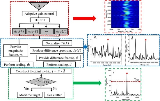
We suggest a method to detect floating maritime targets, even with a short dwell time. The proposed method consists of four steps:
Step 1: Perform automatic gain control (AGC) and extract Doppler spectra of all range bins, , using a 1-D fast Fourier transform (FFT) on radar echoes, .
Step 2: Provide magnitude feature m by calculating the squared-root power of s.
Step 3.a: Conduct power normalization on .
Step 3.b: Employ the difference spectrum , where is the mean Doppler spectrum.
Step 3.c: Provide difference feature d by calculating the power of s.
Step 4: Construct the new joint metric , based on scaled m and d, and determine the range bin using an adaptive statistical detector.
The overall flowchart of the proposed maritime target scheme is illustrated in Figure 1.
3.1. Step1: Range-Doppler Map Formation
First, to compensate for the dependence of receiving power on the distance between radar and target reference, we utilized a simple AGC process on received radar returns . If it is set to have the same antenna gain for all range bins, AGC can be simply defined as:
where denotes the time-series radar signal after AGC received in the th range bin, denotes the distance (i.e., range) corresponding to the th range bin, and denotes the distance for normalization. In this study, we select as the mean distance of all s.
Next, the Doppler spectrum at the th range bin, , is computed using the 1-D FFT on the received time-series signal . If the target moves with a radial velocity , the Doppler spectrum is obtained with a shifted center at as:
i.e.,
where , c, and denote the center frequency of the transmit signal, the velocity of light, and the wavelength of the transmit signal, respectively. In particular, as the observation time T increases to approximately a few seconds, pixel migration for the scatters of fast-moving maritime targets is unavoidable and produces a blurred Doppler spectrum. However, pixel migration may not occur in a short measurement time T of approximately a few milliseconds, even for fast-moving maritime targets. Therefore, for a short dwell time T, the Doppler spectrum with the center frequency of is clearly observed. In particular, the 4 dB resolution of the Doppler spectrum is given by:
As in (17), the short dwell time T inevitably produces large , which is disadvantageous in discrimination of maritime targets from sea clutter, especially for subsequent Step 3. Meanwhile, the frequency spacing and radial velocity spacing in the discretized Doppler spectrum can be induced regardless of T as:
and
K denotes the number of frequency bins in the discretized Doppler spectrum. However, without zero-padding, it should be noted that , resulting in a wide frequency spacing in the discretized Doppler spectrum in the short dwell time T. For this reason, we employ zero-padding for reducing to have , which is the required minimum number of frequency bins, as follows:
where denotes the round-up operator and is the required spacing of radial velocities. Even with the poor from the long T, it can have the fine interval between the peak locations in the Doppler spectrum, via zero-padding.
3.2. Step2: Magnitude Feature
It is widely known that radar echoes from small maritime targets have a larger intensity than non-spiky clutter signals in a wide ocean [24,25]. For this reason, the magnitude (i.e., intensity) of the received signal has been widely used as a feature in maritime target detection [5,26]. To increase the signal-to-clutter ratio (SNR) of the magnitude of the received signal, pulse integration can be adopted to suppress the magnitude of the sea clutter echoes. In this study, we devised a metric based on the magnitude of the received signal, named the magnitude feature (MF) and denoted as m. This is strongly related to the integrated radar echoes with enhanced SNR as follows:
where denotes m at the th range bin. Under Parseval’s theorem, can be produced by calculating the square-root power of . Via integration in (21), m can be regarded as the texture component of sea clutter, which is called local clutter power [24]. The distribution of texture component can be assumed to follow the generalized gamma distribution, as . is the generalized gamma distribution with a PDF given by [27,28]:
denotes the gamma function. and are the shape parameter and the scale parameter for the gamma distribution of m, respectively. The parameter of gamma distribution can be estimated by the method of moments (MoM), which is a commonly used technique for parameter estimation by calculating the lower order moment [25,29].
3.3. Step3: Difference Feature
Even though the MF is useful for maritime target detection, high sea spikes, especially in high sea states, often produce very poor detection results in small maritime target detection, as discussed in [5,6,7,8]. To overcome the drawback of MF only, in this section, we devise another discriminant metric based on the difference between the s of the target and sea clutter, named the difference feature (DF).
In particular, maritime targets, such as small boats and periscopes, are controlled by a pilot and produce their own moving velocity regardless of wave direction. Uncontrolled maritime targets, such as buoys and floating mines, are usually stationary at a certain position in the ocean, even under severe sea conditions (i.e., in a high sea state). For this stationary maritime target, the conventional maritime target detector based on MTI cannot provide the detection performance well. With regard to this characteristic, it can be assumed that the of an interesting maritime target often differs from the of a sea-wave around the target. In other words, the center frequency of the Doppler spectrum of the target is usually far from that of sea-wave .
In this step, DF, denoted as d, is obtained by extracting the difference in the Doppler spectrum of the maritime target bin from those of the sea clutter bins and this feature is devised to find not only moving maritime targets but also stationary ones in moving sea waves. In Step 3.a, the power normalization on is conducted, as represented as:
denotes the normalized Doppler spectrum at the th range bin, and it is carried out repeatedly for all bins, . Via (23), is devised to be independent of the magnitude of the received signal (i.e., MF), thereby performing maritime target detections even at high sea-state conditions. ] is the range-Doppler (RD) map of the normalized spectra, which have the same power regardless of the range bin.
In Step 3.b, we obtain the difference spectrum by subtracting the mean Doppler spectrum and taking the absolute value as:
where:
is the different spectrum at the th range bin and is the mean Doppler spectrum at the th range bin, which is obtained using s at consecutive range bins of . In particular, to cover the successive sea-wave in (25), B is obtained by , where denotes the round operation, is the length of the successive sea-wave in the range dimension, and is the range bin spacing in the RD map.
Furthermore, owing to the spreading wind with a very long fetch length (i.e., wind fetch), the sea-wave is usually successive along the range dimension on the sea [30], resulting in a nearly unchanged at the successive range bins of the sea wave. Hence, the center frequencies of the Doppler spectra of the sea-wave are almost identical and produce a dominant peak at in each sea-wave. In addition, most of the range bins among bins in (25) undoubtedly correspond to sea clutter, thus providing the center frequency of at . As a result, via subtraction in (24), suppression of the peak at is unavoidable for the range bin of sea clutter. This is because the peaks of and that of of sea clutter are located at the same frequency, .
However, owing to the difference between the center frequency of (i.e., ) and that of at a maritime target range bin (i.e., ), not only the peak at but also that at remain in , resulting in two high peaks.
In Step 3.c, d at the th range bin, denoted as , is defined by calculating the power of as follows:
Figure 2 illustrates the procedure of Step 3, with CSIR data based on the x-band radar with PRF = 2 kHz, , and T = 4 ms. In Figure 2a, the normalized RD map has a size of 101 range bins and 114 frequency elements (i.e., K = 114), induced by (20) with = 0.3 m/s. Even with = 250 Hz, it has = 17.5 Hz in (18), thus providing the fine resolution of the peak location. Among the 101 range bins, the 55th range bin belongs to a maritime target bin, and the 35th range bin is one of the sea clutter bins. The solid ellipses in Figure 2a indicate the highest peaks of and corresponding to the maritime target and sea clutter, respectively. Meanwhile, on account of the continuous sea-wave, most s, especially from the sea clutter, has the center of the peaks at approximately 100 Hz. The dashed lines in Figure 2a illustrate the boundaries of the 3 dB width of the Doppler spectrum from the sea-wave. The peak of is located completely inside the boundaries, whereas the location of the peak is almost outside of the boundaries, as shown in Figure 2a.
Figure 2b shows two normalized Doppler spectra, and . , which is for the maritime target and has the highest peak at 168 Hz ( = 2.87 m/s using (16)). Meanwhile, , which is for the sea clutter, provides the highest peak at = 97 Hz (1.66 m/s), which is far from 168 Hz of the maritime target.
Meanwhile, Figure 2c shows the mean Doppler spectra for each range bin with . Both and have a clear and high peak around = 97 Hz. This is because the range bins are surrounded by successive sea-waves with 1.66 m/s.
As shown in Figure 2d, owing to the difference between the locations of high peaks in and , is conferred with two very high peaks at 168 Hz and = 80 Hz. In particular, owing to the deepest valley of at = 80 Hz in Figure 2b, the location of the right-side peak differs slightly from that of at = 97 Hz. On the other hand, and have an identical location of peaks, and therefore produces several very low peaks, as shown in Figure 2d.
As in (26), the two very high peaks in Figure 2d lead to a large in the range bin of the maritime target, whereas the very low peaks in yield a much smaller sea clutter. Furthermore, the PDF of d can be assumed to follow the Gamma distribution ) in (22), which results from the randomly changed by heterogeneous wind [31,32]. This is later demonstrated in Section 4 and Figure 4. Under a sudden strong gust of wind on a certain location, it may produce false peaks at the clutter range bin on d.
3.4. Step4: Proposed Joint Metric
Via Steps 1 to 3, two independent discriminant features, m (i.e., MF) and d (i.e., DF), are extracted from the received signal in the short T. However, both are not robust features for maritime target detection, producing many false peaks. In detail, false peaks in m and those in d may be uncorrelated, therefore located often at different bins. For this reason, we devise a more advanced detection metric via the product of these two features, to suppress the false peaks of sea clutter in either m or d.
Before the product, scaling m and d should be employed to have their PDFs follow each standard gamma distribution, as and . is provided by scaling m to have as the mean value [33], and so does d to produce , as given by:
denotes expectation operator. Using and , we yield a new joint metric j as:
Since we provide the joint metric based on the product of and , the distribution of j can be regarded as a product distribution [34]. , which is the product distribution of two random variables having independent standard gamma distributions, can be defined as [35]:
where:
is the modified Bessel function of the second kind of order v.
Herein, a statistical adaptive threshold for the product distribution can be determined by the following equation:
is a constant false alarm rate, which is determined a priori by the user. With a numerical calculation, the statistical adaptive threshold can be achieved. Finally, each range bin with j is assigned to one of two classes.
With the suppressed false peaks in , it can result in a robust detection performance.
Figure 3 illustrates , , and j for the 101 range bins from the data used in Figure 2. The peaks marked as “ * ” indicate the values at the target bin, that is, the 55th bin. The red dashed lines indicate the adaptive thresholds induced by the CFAR detector with an identical false alarm rate, .
Figure 3a shows the plot of for 101 range bins with a calculated threshold, , which is based on a gamma distribution as in (23) with . can be employed to discriminate the maritime target bin from sea clutter, even in the short T. However, it is observed that there are still many sea spikes owing to either a small-sized floating target or strong sea clutter, often causing many false alarms.
Meanwhile, Figure 3b exhibits not only the plot of for 101 range bins having very high peaks at the 21th and 55th bins, but also the CFAR threshold, , based on the gamma distribution with . Most of the range bins corresponding to sea clutter have a small , resulting from clutter suppression by Step 2. It can be shown that maritime target detection using is conducted with fine detection results. However, abnormal Doppler spectra of sea clutter due to a local gust of wind can occur, thus leading to false peaks, such as the peak at the 21th range bin, as shown in Figure 3b.
As presented in Figure 3c, it is clear that the peak of j at the range bin (i.e., ) is quite suppressed via the production of and , especially compared with in Figure 3b. However, the peak in j for the maritime target (i.e., ) is still high. In terms of detection performance induced in (31), this proposed scheme provides the best and improved performance in maritime target detection.
4. Experimental Results
4.1. Performance Metric
To evaluate the detection performance of the proposed joint metric, we conducted an experiment using CSIR. In particular, we compared the detection capabilities based on four different discriminant metrics: (1) The proposed joint metric, (2) the power extracted by the EMD technique, (3) the Hurst parameter by fractal analysis, and (4) the error estimated by the neural network using RBF, as addressed in Section II-B. For the sake of notational brevity, in the following detection experiments, we refer to the proposed joint metric as “J,” the metric based on EMD as “EMD,” that metric based on fractal analysis as “Fractal,” and the metric based on the neural network using RBF as “RBF-NN.”
The detection performance indicators in this experiment are the ASCR, detection rate (true-positive rate), false alarm rate (false-positive rate), and processing time.
Firstly, ASCR is calculated as [36]:
where and are the averaged power of the target and sea clutter, respectively. Furthermore, denotes an expectation operator, denotes the discriminant metric from each detector—that is, (1) the proposed joint metric, (2) the power extracted by the EMD technique, (3) the Hurst parameter by fractal analysis, and (4) the error estimated by the neural network using the RBF—of the maritime target bins. Moreover, denotes those from the range bins of sea clutter. If the target signal becomes stronger, the ASCR becomes larger, thereby obviously leading to better performance in terms of the detection rate. As a result, in this experiment, ASCR was adopted as an evaluation metric for assessing detection performance.
The other indicators, the detection rate, and the false alarm rate in the range bin unit, are carried out as [37]:
where is the total number of target bins, and denotes the number of detected target bins. Meanwhile, and are the total number of bins of sea clutter and the number of detected clutter bins, respectively.
4.2. Evaluation of Detection Performance Using Real Measured CSIR Data
In this section, we evaluate the detection performance of the maritime target detector using real measured radar data. We chose radar data, which were obtained by a team led by Herselman of the CSIR. This team collected real data on sea clutter and floating maritime targets, such as small boats, in 2007. The data were collected at Cape Town Harbor in South Africa using a radar deployed on Signal Hill [21]. In this experiment, five datasets of the CSIR datasets were selected, operating with a carrier frequency of 8.8 GHz and a range sampling interval of 15 m in HH polarization. Other specific parameters for the five datasets are listed in Table 1. Each dataset was composed of thousands of radar echoes measured in long T (approximately 30–90 s).
In this study, we randomly selected 200 samples of the short T in each dataset. Each sample was composed of successive radar echoes of the short, whose range is T = [5 ms, 10 ms, 15 ms, 20 ms, and 25 ms]. The range of T was selected from those widely applied in recent surveillance radars, as mentioned in section II-A. Consequently, the total number of samples in this experiment was 3 datasets × 200 samples × 5 different Ts = 3000 samples.
Figure 4 shows the fitting results of “00-011”, “00-012”, and “00-017”, respectively, illustrating PDFs of d (solid lines), Rayleigh (solid lines with circles), Log-normal (solid lines with diamond), Normal (dotted lines), and Gamma (dashed lines) distributions. It is shown that the Gamma distribution obviously fits to the PDF of d, compared to the other PDFs. The parameters of the distributions are estimated by MoM methods. Furthermore, Table 2 summarizes the fitting error value obtained by the chi-squared test [38]. from Gamma distribution is the smallest among the values in Table 2-new, which indicates that the Gamma distribution is best fitted with the PDF of d.
Figure 5 shows the fitting results with PDFs of j (solid lines) and (dashed lines) based on “00-011,” “00-012,” and “00-017,” respectively. Figure 5a depicts the PDF of j from “00-011” with a good fit result obtained by . The fitting result using the dataset ‘00-012’ is illustrated in Figure 5b, which shows good matching results for the PDF of j and with and . In Figure 5c, it is clearly shown that j obtained from ‘00-017’ provides the PDF with the shape of the product distribution of and . In short, it can be found that the PDF of J follows the product distribution of gamma distributions, , not only mathematically, as in (29), but also experimentally, as shown in Figure 5.
Figure 6 shows the plots of ASCR in the decibel scale at each for all four detectors, “J” (solid line), “EMD” (dotted line), “Fractal” (solid line with marker “ ∘ ”), and “RBF-NN” (solid line with marker “*”). In this experiment, for the proposed detector, we assigned = 0.5 [m/s] in (20) and in (25), obtained by = 500 m and = 15 m. In addition, we chose in (5) for “Fractal,” and in (10) for “RBF-NN.”
Figure 6a shows the plots of ASCR in the range of T = [5 ms–25 ms], based on the dataset “00-011.” The ASCRs of “J” and “EMD” remain nearly unchanged, regardless of T. Meanwhile, the ASCRs of “Fractal” and “RBF-NN” obviously increase as T increases however, they provide much lower ASCRs than those of “J” and “EMD” in the considered range of T. Specifically, “J” and “EMD” produce a nearly 7 dB higher ASCR than those of “Fractal” and “RBF-NN at T = 5 ms, a nearly 2 dB higher ASCR than that of “RBF-NN,” and 6 dB higher than that of “Fractal” at T = 25 ms.
In Figure 6b, the plots of ASCR versus T for the dataset “00-012” are shown. The ASCRs of “EMD,” and “Fractal” are unchanged irrespective of T, whereas those of “RBF-NN” drastically increase as T increases. Meanwhile, it is observed that “J” yields a slightly decreasing ASCR along T, providing that ASCR = 7.7 dB at T = 5 ms and ASCR = 6.4 dB at T = 25 ms. Despite this slight decrease, the proposed joint metric produces much higher ASCRs in the considered range of T compared to those from the others.
Figure 6c shows the detection result using the dataset “00-017,” indicating the best performance (i.e., the highest ASCR) of “J” among the four detection techniques. “RBF-NN” and “Fractal” have an increasing ASCR over T but are much lower than “J”. Even for the longest T in the range (i.e., T = 25 ms), “J” produces a nearly 3 dB higher ASCR than that of “RBF-NN” and 7 dB higher than “Fractal.” The plot corresponding to “EMD” is nearly unchanged, although it is nearly 3.5 dB lower than “J”.
In Figure 7a, the plots for the mean value of the ASCR using all datasets above (i.e., 3000 samples) are illustrated. “EMD” produces nearly unchanged ASCRs regardless of T however, the ASCR of “EMD” is nearly 3 dB lower than that of “J” in the considered range of T. In addition, “Fractal” provides a nearly 11 dB lower ASCR than “J”, despite the slight increase as T increases. Meanwhile, it is clearly shown that the ASCR of the “RBF-NN” drastically increases as T increases. However, in the considered range of T, which is adopted for recent marine surveillance radar, “RBF-NN” a such poor performance in terms of ASCR. Contrary to these conventional detectors, it is obvious that the proposed “J” produces the highest ASCR in the considered range of T.
Meanwhile, the ASCR of “J” decreases slightly as T increases. To investigate this degradation, we analyzed ASCRs of and versus T, respectively, as shown in Figure 7b. In fact, it represents the ASCRs of m and d, as well. The ASCR of m slightly increases as T increases, which may result from the integration with the increasing number of radar echoes, . Whereas, it is observed that the ASCR of d decreases slightly as T increases.
In Figure 8, the degradation in d (i.e., ) was investigated by illustrating the RD maps in different Ts, T = 5 ms and T = 25 ms. The solid ellipses indicate the highest peaks of and at the target bin, respectively. In Figure 8a,b, those in T = 5 ms are shown, respectively. With T = 5 ms, = 200 Hz is induced, as in (17). On the other hand, in Figure 8c,d, those in T = 25 ms provide much smaller = 40 Hz, which is usually regarded as an advantage in discrimination. However, the remained peaks of in T = 5 ms would offer a larger d, compared to those of T = 25 ms, especially at the target bins. Whereas, regardless of (i.e., T), the peaks of s at clutter bins are totally suppressed via (24), in ideal. Therefore, in terms of d, it results in a better performance in T = 5 ms than that in T = 25 ms.
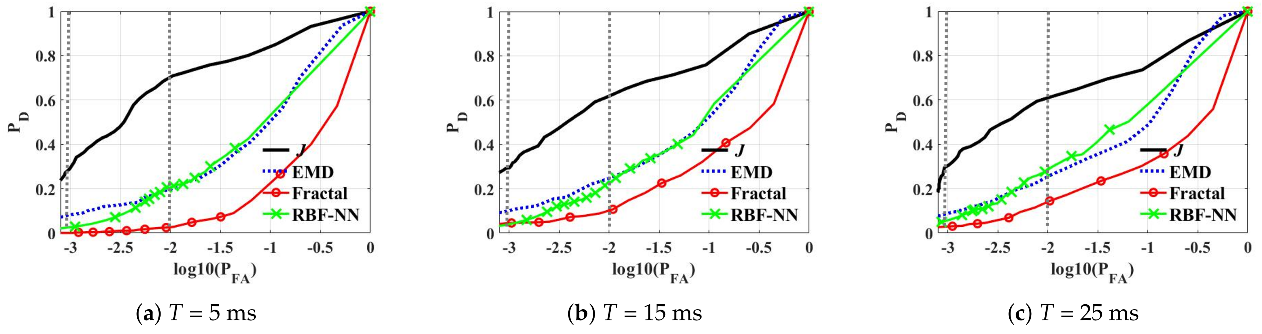
In addition, we conducted further experiments in terms of and , with plotting receiver operating characteristic (ROC) curves. Figure 8 shows the ROC curves of four different maritime target detectors in terms of on a linear scale and on a decibel scale based on the three Ts (T = 5 ms, T = 15 ms, and T = 25 ms). As shown in the three figures in Figure 8, the plots of “J” is the closest to the upper left corner. It implies that the proposed detector provides the higher compared to those of the other conventional detectors, at the range of . Therefore, it is clearly observed that “J” performs much better than the conventional ones, in the considered range of T. Furthermore, Table 3 and Table 4 summarize the results of these four detectors at and , which are the intersecting points of the dashed vertical lines and the ROC curves in Figure 9. As shown in Table 3 for , of “J” in T = 25 ms is 0.684, which is much higher than those of the conventional detectors. Even in the longer T, such as T = 15 ms and T = 25 ms, “J” provides much higher values than the others. In the case of , as in Table 4, “J” produces a much higher than the conventional detectors. Specifically, of the conventional detectors increases as T increases, as in Table 3 and Table 4 however, they have much worse detection performance in the considered range of T than “J”.
Finally, we compared the maritime target detectors in terms of computation time. The running time was measured using MATLAB R2019 and a PC with an Intel i7–9700 K CPU processor and 64 GB RAM. Table 5 summarizes the processing time for different maritime target detectors. The proposed detector “J” requires a processing time of about 26 milliseconds. Due to the numerical calculation on (31), this proposed detector requires a slightly longer processing time than those of "RBF-NN", whereas, it is obviously shorter than those of "EMD" and "Fractal". Therefore, as shown in Figure 6 and Figure 9, and Table 3 and Table 4, the proposed maritime target detector based on the new joint metric performs considerably better than the conventional detectors in terms of ASCR and , with quite a short processing time.
5. Conclusions
In this paper, we proposed a new maritime target detector that provides robust performance in a short dwell time, which is usually inevitable in recent marine surveillance radars. The proposed detector uses a new joint metric obtained by the product of the scaled magnitude and difference features, whose scale parameters are adjusted to be one. The difference feature is fundamentally based on the target radial velocities that are different from those around the sea wave, devised to detect both stationary and moving maritime targets. Since the PDF of the joint metric follows the product distribution of standard gamma distributions, we adopted an adaptive threshold on the joint metric under and a priori-determined false alarm rate. Our experimental results using the CSIR dataset showed that the proposed metric can provide stable and much better maritime target performance in terms of the ASCR and detection rate compared to conventional techniques, such as “EMD”, “Fractal”, and “RBF-NN”. Furthermore, it requires a comparatively short processing time, which enables real-time marine surveillance radar for defense and rescue. It is worth noting that it is straightforward to extend the proposed scheme to combine it with other discriminant features from the maritime target.
Author Contributions
M.-J.L. proposed the idea of the method and wrote the paper; J.-E.K. and B.-H.R. conceived and designed the experiments; K.-T.K. analyzed the data. All authors have approved the contents of the submitted manuscript.
Funding
This research received no external funding.
Institutional Review Board Statement
Not applicable.
Informed Consent Statement
Not applicable.
Data Availability Statement
For the results and data generated during the study, please contact the first author.
Acknowledgments
This research was supported by the the BK21 FOUR program. In addition, the authors would like to thank the reviewers for their valuable comments on this paper.
Conflicts of Interest
The authors declare no conflict of interest.
References
- Kim, J.E.; Lee, S.M.; Kim, C.H.; Kim, Y.S.; Lee, S.J.; Kim, K.T.; Kim, H.J.; Park, S.K. Effect of range resolution in the analysis of X-band sea clutter at low grazing angles. J. Electromagn. Waves Appl. 2019, 33, 2513–2528. [Google Scholar] [CrossRef]
- Rosenberg, L.; Bocquet, S. The Pareto distribution for high grazing angle sea-clutter. In Proceedings of the 2013 IEEE International Geoscience and Remote Sensing Symposium-IGARSS, Melbourne, VIC, Australia, 21–26 July 2013; pp. 4209–4212. [Google Scholar]
- Zhou, W.; Xie, J.; Zhang, B.; Li, G. Maximum likelihood detector in gamma-distributed sea clutter. IEEE Geosci. Remote Sens. Lett. 2018, 15, 1705–1709. [Google Scholar] [CrossRef]
- Zhao, J.; Jiang, R.; Wang, X.; Gao, H. Robust CFAR detection for multiple targets in K-distributed sea clutter based on machine learning. Symmetry 2019, 11, 1482. [Google Scholar] [CrossRef] [Green Version]
- Shui, P.L.; Li, D.C.; Xu, S.W. Tri-feature-based detection of floating small targets in sea clutter. IEEE Trans. Aerosp. Electron. Syst. 2014, 50, 1416–1430. [Google Scholar] [CrossRef]
- Shi, S.N.; Shui, P.L. Sea-surface floating small target detection by one-class classifier in time-frequency feature space. IEEE Trans. Geosci. Remote Sens. 2018, 56, 6395–6411. [Google Scholar] [CrossRef]
- Hu, J.; Tung, W.W.; Gao, J. Detection of low observable targets within sea clutter by structure function based multifractal analysis. IEEE Trans. Antennas Propag. 2006, 54, 136–143. [Google Scholar] [CrossRef]
- Luo, F.; Zhang, D.; Zhang, B. The fractal properties of sea clutter and their applications in maritime target detection. IEEE Geosci. Remote Sens. Lett. 2013, 10, 1295–1299. [Google Scholar] [CrossRef]
- Chunsheng, X.; Hao, C.; Dong, X. Sea clutter characteristics analysis and target detection based on HHT. In Proceedings of the 2011 International Conference on Consumer Electronics, Communications and Networks (CECNet), Xianning, China, 16–18 April 2011; pp. 694–697. [Google Scholar]
- McDonald, M.K.; Cerutti-Maori, D. Coherent radar processing in sea clutter environments, part 2: Adaptive normalised matched filter versus adaptive matched filter performance. IEEE Trans. Aerosp. Electron. Syst. 2016, 52, 1818–1833. [Google Scholar] [CrossRef]
- Orlando, D.; Venturino, L.; Lops, M.; Ricci, G. Track-before-detect strategies for STAP radars. IEEE Trans. Signal Process. 2009, 58, 933–938. [Google Scholar] [CrossRef]
- Davey, S.J.; Rutten, M.G.; Cheung, B. A comparison of detection performance for several track-before-detect algorithms. EURASIP J. Adv. Signal Process. 2007, 2008, 1–10. [Google Scholar] [CrossRef] [Green Version]
- Yujie, L.; Wenguang, W.; Jinping, S. Research of small target detection within sea clutter based on chaos. In Proceedings of the 2009 International Conference on Environmental Science and Information Application Technology, Wuhan, China, 4–5 July 2009; Volume 2, pp. 469–472. [Google Scholar]
- Hennessey, G.; Leung, H.; Drosopoulos, A.; Yip, P.C. Sea-clutter modeling using a radial-basis-function neural network. IEEE J. Ocean. Eng. 2001, 26, 358–372. [Google Scholar] [CrossRef]
- Gao, J.; Yao, K. Multifractal features of sea clutter. In Proceedings of the 2002 IEEE Radar Conference (IEEE Cat. No. 02CH37322), Long Beach, CA, USA, 25 April 2002; pp. 500–505. [Google Scholar]
- Orlando, D.; Ehlers, F.; Ricci, G. Track-before-detect algorithms for bistatic sonars. In Proceedings of the 2010 2nd International Workshop on Cognitive Information Processing, Elba, Italy, 14–16 June 2010; pp. 180–185. [Google Scholar]
- Orlando, D.; Ricci, G.; Bar-Shalom, Y. Track-before-detect algorithms for targets with kinematic constraints. IEEE Trans. Aerosp. Electron. Syst. 2011, 47, 1837–1849. [Google Scholar] [CrossRef]
- Bole, A.G.; Wall, A.D.; Norris, A. Radar and ARPA Manual: Radar, AIS and Target Tracking for Marine Radar Users; Butterworth-Heinemann: Oxford, UK, 2013. [Google Scholar]
- Nieto-Borge, J.; Hessner, K.; Jarabo-Amores, P.; De La Mata-Moya, D. Signal-to-noise ratio analysis to estimate ocean wave heights from X-band marine radar image time series. IET Radar Sonar Navig. 2008, 2, 35–41. [Google Scholar] [CrossRef] [Green Version]
- Miranda, S.; Baker, C.; Woodbridge, K.; Griffiths, H. Knowledge-based resource management for multifunction radar: A look at scheduling and task prioritization. IEEE Signal Process. Mag. 2006, 23, 66–76. [Google Scholar] [CrossRef] [Green Version]
- Herselman, P.; Baker, C.; De Wind, H. Analysis of X-band calibrated sea clutter and small boat reflectivity at medium-to-low grazing angles. Int. J. Navig. Obs. 2008, 2008. [Google Scholar] [CrossRef] [Green Version]
- Guangran, X.; Zicheng, D.; Wei, W.; Lang, H. Multi-beam dwell adaptive scheduling algorithm for helicopter-borne radar. In Proceedings of the 2014 IEEE 7th Joint International Information Technology and Artificial Intelligence Conference, Chongqing, China, 20–21 December 2014l; pp. 401–404. [Google Scholar]
- Huang, N.E.; Shen, Z.; Long, S.R.; Wu, M.C.; Shih, H.H.; Zheng, Q.; Yen, N.C.; Tung, C.C.; Liu, H.H. The empirical mode decomposition and the Hilbert spectrum for nonlinear and non-stationary time series analysis. Proc. R. Soc. Lond. Ser. A Math. Phys. Eng. Sci. 1998, 454, 903–995. [Google Scholar] [CrossRef]
- Watts, S. Modeling and simulation of coherent sea clutter. IEEE Trans. Aerosp. Electron. Syst. 2012, 48, 3303–3317. [Google Scholar] [CrossRef]
- Zhou, W.; Xie, J.; Li, G.; Du, Y. Robust CFAR detector with weighted amplitude iteration in nonhomogeneous sea clutter. IEEE Trans. Aerosp. Electron. Syst. 2017, 53, 1520–1535. [Google Scholar] [CrossRef]
- Watts, S.; Baker, C.; Ward, K. Maritime surveillance radar. Part 2: Detection performance prediction in sea clutter. In IEE Proceedings F (Radar and Signal Processing); IET: London, UK, 1990; Volume 137, pp. 63–72. [Google Scholar]
- Ward, K.D.; Watts, S.; Tough, R.J. Sea Clutter: Scattering, the K Distribution and Radar Performance; IET: London, UK, 2006; Volume 20. [Google Scholar]
- Ugarte, L.S.; de Miguel Vela, G.; Portas, J.A.B. Simulation model for sea clutter in airborne radars. In Proceedings of the 2011 8th European Radar Conference, Manchester, UK, 12–14 October 2011; pp. 77–80. [Google Scholar]
- Skolnik, M.I. Introduction to Radar Systems; McGraw-hill: New York, NY, USA, 1962; Volume 3. [Google Scholar]
- Wikipedia Contributors. Wind Wave—Wikipedia, The Free Encyclopedia. 2021. Available online: https://en.wikipedia.org/wiki/Wind_wave (accessed on 24 February 2021).
- Kiss, P.; Jánosi, I.M. Comprehensive empirical analysis of ERA-40 surface wind speed distribution over Europe. Energy Convers. Manag. 2008, 49, 2142–2151. [Google Scholar] [CrossRef]
- Kollu, R.; Rayapudi, S.R.; Narasimham, S.; Pakkurthi, K.M. Mixture probability distribution functions to model wind speed distributions. Int. J. Energy Environ. Eng. 2012, 3, 1–10. [Google Scholar] [CrossRef] [Green Version]
- Wikipedia Contributors. Gamma Distribution—Wikipedia, The Free Encyclopedia. 2021. Available online: https://en.wikipedia.org/wiki/Gamma_distribution (accessed on 18 March 2021).
- Wikipedia Contributors. Product Distribution—Wikipedia, The Free Encyclopedia. 2021. Available online: https://en.wikipedia.org/wiki/Product_distribution (accessed on 18 March 2021).
- Withers, C.S.; Nadarajah, S. On the product of gamma random variables. Qual. Quant. 2013, 47, 545–552. [Google Scholar] [CrossRef]
- Shui, P.; Guo, Z.; Shi, S. Feature-compression-based detection of sea-surface small targets. IEEE Access 2019, 8, 8371–8385. [Google Scholar] [CrossRef]
- Lee, M.J.; Kim, J.E.; Lee, S.M.; Ryu, B.H.; Kim, K.T. A study on modeling of sea clutter echo for short time of measurement. In Proceedings of the 8th Asia-Pacific Conference on Antennas Propagation, Incheon, South Korea, 4–7 August 2019; pp. 1–2. [Google Scholar]
- Satorra, A.; Bentler, P.M. A scaled difference chi-square test statistic for moment structure analysis. Psychometrika 2001, 66, 507–514. [Google Scholar] [CrossRef] [Green Version]
Figure 1.
Flowchart illustrating steps of the proposed maritime target detector.

Figure 2.
Doppler spectra of the target range bin and a clutter bin.
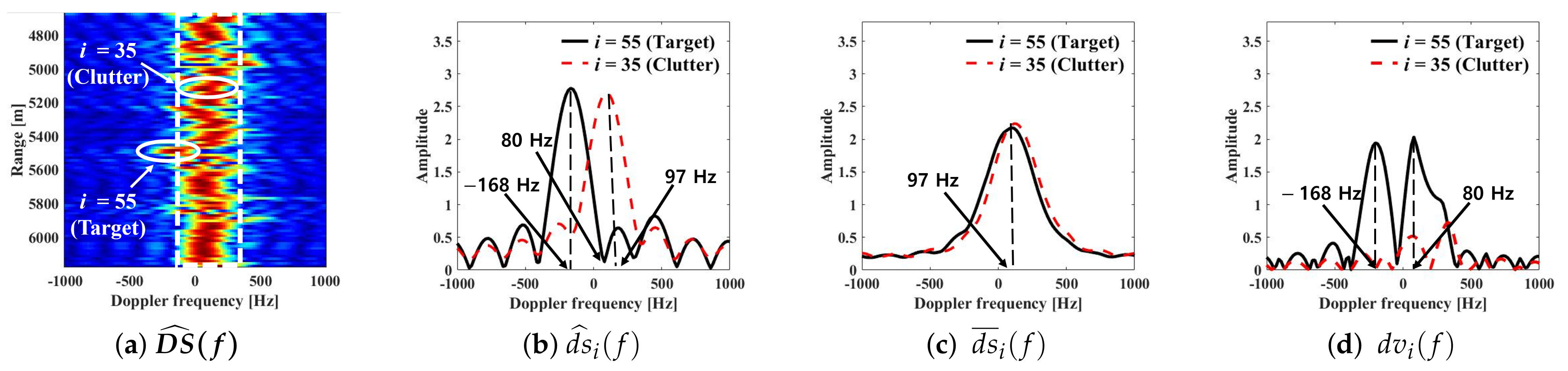
Figure 3.
Discriminant feature of a target range bin (55th range bin) and clutter ones.

Figure 4.
Comparison of the probability density function (PDF) of d with four distributions.
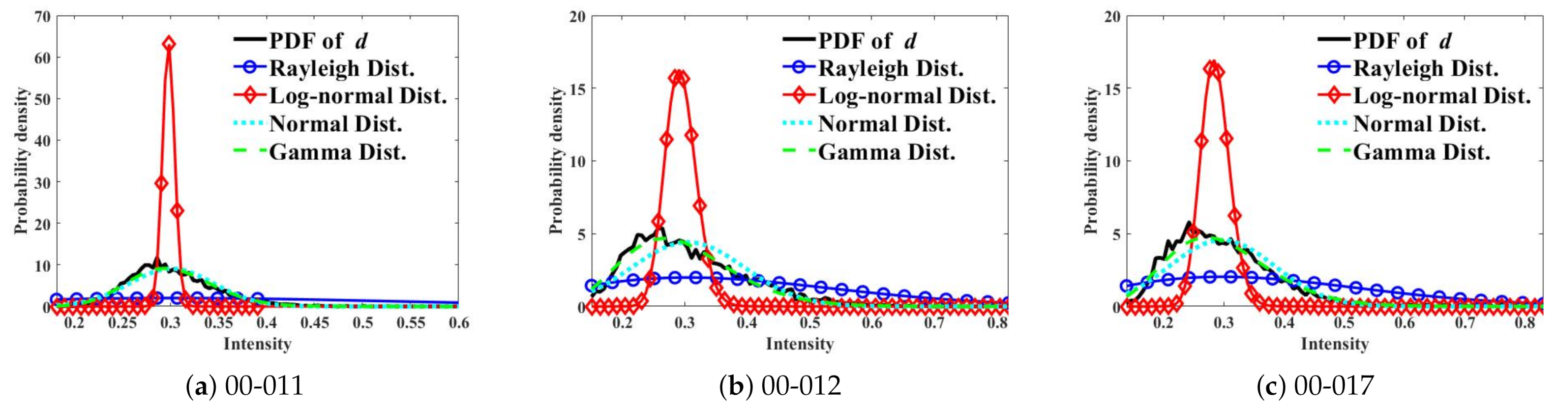
Figure 5.
Comparison of the PDF of j with ).
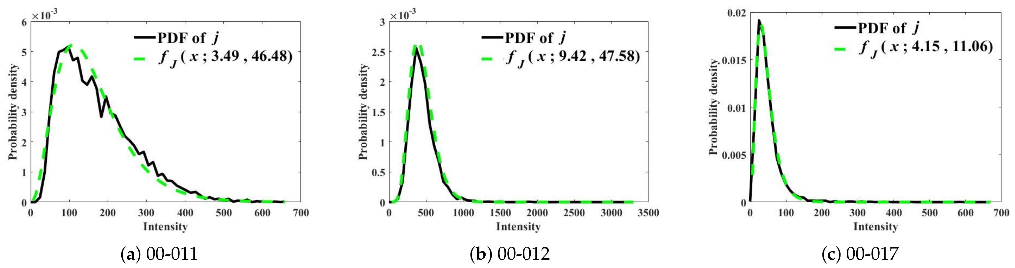
Figure 6.
Mean value of average signal-to-clutter ratio (ASCR) versus T using each dataset.

Figure 7.
Mean value of ASCR versus T using all datasets.

Figure 8.
RD maps of and in two different Ts.
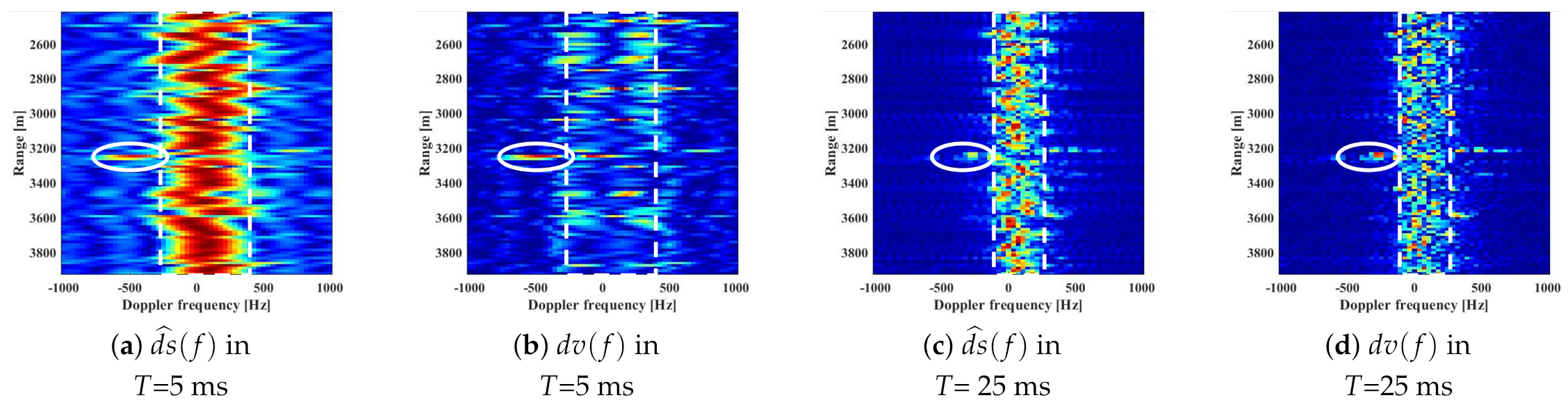
Figure 9.
Detection results using ROC curves.

Table 1.
Description of data sets used.
| File Name | Range (m) / # of Range-Bins | Tracking Range (m) | Total Duration Time (sec) | Sea State | Wave Direction () | PRF (kHz) | Grazing Angle () |
|---|---|---|---|---|---|---|---|
| 00-011 | 1499/101 | 2274.4 | 34.22 | 4.5 | 261.7 | 2.0 | 4.67–7.78 |
| 00-012 | 1499/101 | 2424.3 | 29.50 | 4.5 | 261.7 | 2.0 | 4.67–7.78 |
| 00-017 | 1499/101 | 4672.8 | 49.17 | 4.5 | 261.7 | 2.0 | 2.84–3.76 |
Table 2.
Fitting error using Chi-Squared test on d in Figure 4.
Table 2.
Fitting error using Chi-Squared test on d in Figure 4.
| File Name | ||||
|---|---|---|---|---|
| Rayleigh | Log-Normal | Normal | Gamma | |
| 00-011 | 9.64 | 12.83 | 0.17 | 0.06 |
| 00-012 | 2.37 | 2.63 | 0.31 | 0.14 |
| 00-017 | 3.80 | 3.19 | 0.37 | 0.14 |
Table 3.
of detectors in various T at . (EMD: empirical mode decomposition, RBF-NN: radial basis function-based neural network).
Table 3.
of detectors in various T at . (EMD: empirical mode decomposition, RBF-NN: radial basis function-based neural network).
| Detectors | |||
|---|---|---|---|
| T = 5 ms | T = 15 ms | T = 25 ms | |
| J | 0.684 | 0.640 | 0.639 |
| EMD | 0.198 | 0.248 | 0.253 |
| Fractal | 0.027 | 0.100 | 0.142 |
| RBF-NN | 0.204 | 0.230 | 0.285 |
Table 4.
of detectors in various T at .
| Detectors | |||
|---|---|---|---|
| T = 5 ms | T = 15 ms | T = 25 ms | |
| J | 0.296 | 0.295 | 0.295 |
| EMD | 0.083 | 0.102 | 0.109 |
| Fractal | 6.08 × 10 | 0.045 | 0.050 |
| RBF-NN | 0.018 | 0.046 | 0.061 |
Table 5.
Processing time of each detector in various T.
| Detectors | Processing Time [ms] | ||||
|---|---|---|---|---|---|
| T = 5 ms | T = 10 ms | T = 15 ms | T = 20 ms | T = 25 ms | |
| J | 26.6 | 26.4 | 26.3 | 26.2 | 26.2 |
| EMD | 296.3 | 418.0 | 545.0 | 599.1 | 691.3 |
| Fractal | 86.3 | 87.8 | 89.3 | 96.5 | 99.1 |
| RBF-NN | 5.6 | 9.8 | 12.5 | 26.9 | 31.9 |
Publisher’s Note: MDPI stays neutral with regard to jurisdictional claims in published maps and institutional affiliations. |
© 2021 by the authors. Licensee MDPI, Basel, Switzerland. This article is an open access article distributed under the terms and conditions of the Creative Commons Attribution (CC BY) license (https://creativecommons.org/licenses/by/4.0/).
Share and Cite
MDPI and ACS Style
Lee, M.-J.; Kim, J.-E.; Ryu, B.-H.; Kim, K.-T. Robust Maritime Target Detector in Short Dwell Time. Remote Sens. 2021, 13, 1319. https://doi.org/10.3390/rs13071319
AMA Style
Lee M-J, Kim J-E, Ryu B-H, Kim K-T. Robust Maritime Target Detector in Short Dwell Time. Remote Sensing. 2021; 13(7):1319. https://doi.org/10.3390/rs13071319
Chicago/Turabian StyleLee, Myung-Jun, Ji-Eun Kim, Bo-Hyun Ryu, and Kyung-Tae Kim. 2021. "Robust Maritime Target Detector in Short Dwell Time" Remote Sensing 13, no. 7: 1319. https://doi.org/10.3390/rs13071319
Note that from the first issue of 2016, this journal uses article numbers instead of page numbers. See further details here.