
Potential of Hybrid CNN-RF Model for Early Crop Mapping with Limited Input Data
by
 ,
,
Geun-Ho Kwak
1 ,
,
Chan-won Park
2,
Kyung-do Lee
3,
Sang-il Na
3,
Ho-yong Ahn
3 and 
No-Wook Park
1,*
1
Department of Geoinformatic Engineering, Inha University, Incheon 22212, Korea
2
Research Policy Bureau, Rural Development Administration, Jeonju 54875, Korea
3
National Institute of Agricultural Sciences, Rural Development Administration, Wanju 55365, Korea
*
Author to whom correspondence should be addressed.
Remote Sens. 2021, 13(9), 1629; https://doi.org/10.3390/rs13091629
Submission received: 8 March 2021
/
Revised: 15 April 2021
/
Accepted: 19 April 2021
/
Published: 21 April 2021
(This article belongs to the Special Issue Selected Papers from the “International Symposium on Remote Sensing 2021”)
Abstract
:When sufficient time-series images and training data are unavailable for crop classification, features extracted from convolutional neural network (CNN)-based representative learning may not provide useful information to discriminate crops with similar spectral characteristics, leading to poor classification accuracy. In particular, limited input data are the main obstacles to obtain reliable classification results for early crop mapping. This study investigates the potential of a hybrid classification approach, i.e., CNN-random forest (CNN-RF), in the context of early crop mapping, that combines the automatic feature extraction capability of CNN with the superior discrimination capability of an RF classifier. Two experiments on incremental crop classification with unmanned aerial vehicle images were conducted to compare the performance of CNN-RF with that of CNN and RF with respect to the length of the time-series and training data sizes. When sufficient time-series images and training data were used for the classification, the accuracy of CNN-RF was slightly higher or comparable with that of CNN. In contrast, when fewer images and the smallest training data were used at the early crop growth stage, CNN-RF was substantially beneficial and the overall accuracy increased by maximum 6.7%p and 4.6%p in the two study areas, respectively, compared to CNN. This is attributed to its ability to discriminate crops from features with insufficient information using a more sophisticated classifier. The experimental results demonstrate that CNN-RF is an effective classifier for early crop mapping when only limited input images and training samples are available.
1. Introduction
The demand for timely and accurate agricultural thematic information has been increasing in the agricultural community owing to increased food security needs and climatic disasters [1,2,3]. In particular, crop type information is considered to be vital for sustainable agricultural monitoring and management [4]. Conventional official agricultural statistics, including the cultivation areas and crop yields, have been widely used to support agricultural planning and management. However, from a practical perspective, such statistics may not be useful for the preemptive establishment of national food policies as it is usually released either after crop seasons or on a simple annual basis. Therefore, crop type information should be provided to decision-makers either before crop seasons or at a time desirable for effective agricultural management [5,6].
Remote sensing technology has been widely employed to generate crop type maps at both local and regional scales owing to its ability to provide useful information for the periodic monitoring and effective management of agricultural fields [7,8]. However, the accurate classification of crop types using remote sensing imagery still poses challenges, particularly for early crop mapping, as certain important aspects for crop classification should be properly considered during the classification procedure. Time-series remote sensing images acquired during the growth cycles of crops of interest are usually used as the input for classification to account for the temporal variations in the spectral and scattering characteristics of crop types [9,10]. When an incomplete time-series image set that cannot account for the full growth cycles of crops is used for the classification, distinguishing various crops with similar spectral responses is often difficult, thus achieving relatively poor classification performance. From a practical perspective, however, there is still a demand for generating crop type maps using only the images collected during the early crop growth period as decision-makers require such maps before the end of the crop seasons [11,12]. For crop type maps generated from an incomplete time-series set to be practically useful, achieving a classification performance comparable with that generated from a complete time-series set is necessary.
Another important challenge in crop classification using remote sensing imagery is collecting the sufficient training data useful for crop identification, which is common in the supervised classification of remote sensing imagery [13,14]. However, collecting sufficient training data for supervised classification is costly and time-consuming. When an incomplete time-series set is used for early crop mapping, particularly, it may be difficult to collect informative training data, with the quantity and quality of training data greatly affecting the classification performance [12].
When only limited remote sensing images and training data are available for classification, selecting an optimal classification model is critical to achieve a satisfactory classification performance. Machine learning (ML) algorithms, including artificial neural network (ANN), random forests (RF), and support vector machine (SVM), have been widely applied for the classification of remote sensing images because of their ability to satisfactorily quantify nonlinear decision boundaries [15,16,17,18]. Furthermore, to account for the spatial patterns or features implicit in an image of interest during classification, a feature extraction and selection stage is combined with conventional ML models [4,19]. However, the extraction and selection of optimal features may be time-consuming, and considerable effort is required prior to classification [20].
In recent years, researchers in remote sensing communities have become increasingly interested in deep learning (DL) for image classification [21,22,23,24,25] and object detection [26,27]. Compared with ML models, DL models can automatically extract high-level features from input images without user intervention [28]. To effectively account for the temporal contextual information from time-series images, recurrent neural network (RNN) and its variants, including long short-term memory (LSTM), have been applied to crop mapping [29,30]. However, the classification performance of such RNN-type DL models for early crop mapping may be unsatisfactory because of the temporal information deficiency from the incomplete time-series set. To overcome the limitation of insufficient temporal contextual information, convolutional neural network (CNN) that considers complex spatial patterns between neighboring pixels within a patch is efficient for classifying regions with similar spectral and spatial characteristics such as agricultural fields [24,25]. For example, the superiority of CNN in crop classification has been verified through comparisons with conventional ML and other DL models [9,10,11,31,32]. However, training the CNN model with limited information, in terms of the quantity and quality of training data as well as the length of the input time-series, is still challenging [33].
The performance of classification with limited inputs can be improved by applying a hybrid model with multiple classifiers where each individual classifier exhibits complementary behavior [34,35,36]. The combination of the DL model with the ML model can achieve better classification accuracy than each single model. The former can extract informative spatial features automatically, and the latter can properly determine nonlinear decision boundaries from the extracted features. Such a hybrid model combining a CNN as a feature extractor with RF as a sophisticated classifier (herein referred to as CNN-RF) has been proposed for the supervised classification. Moreover, its effectiveness when insufficient information is used for the learning process is demonstrated, compared with conventional CNN that is susceptible to overfitting problems due to input information deficiency [35,36,37,38]. Thus, CNN-RF is promising when limited input data are available for early crop mapping. However, to the best of our knowledge, the full potential of CNN-RF has not yet been thoroughly explored in existing studies for early crop mapping with both limited input images and insufficient training data. Instead of applying advanced models, most previous studies on early crop mapping have focused on either the construction of a sufficient time-series SAR image set [11], or the fusion of optical and SAR images [39]. Yang et al. [35] applied CNN-RF for crop classification with multi-temporal Sentinel-2 images but focused on the selection of optimal features. Furthermore, the lack of sufficient training data has not been investigated in conjunction with different time-series lengths.
The objective of this study is to evaluate the potential of a hybrid CNN-RF model for early crop classification. This study differs from previous ones on the classification using CNN-RF by considering practical issues frequently encountered in early crop mapping, including both the incomplete time-series set and the insufficient training data. The benefit of CNN-RF is quantitatively evaluated by incremental classification experiments using multi-temporal unmanned aerial vehicle (UAV) images and different sizes of training data in two crop cultivation areas in Korea, with an emphasis on early crop mapping.
2. Study Areas and Datasets
2.1. Study Areas
Crop classification experiments were conducted in two major crop cultivation areas in Korea. The first case study area is located in the central part of Anbandegi, a major highland Kimchi cabbage cultivation area in Korea (Figure 1a). The altitude of the study area is relatively higher than its surroundings (1 km above the mean sea level) because low temperatures are required during summer for growing highland Kimchi cabbage [4]. Two other crops, including cabbage and potato, are also grown in the study area, and some fields are managed as fallow which is left without sowing for the following year’s cultivation. The total area of all crop parcels is 27.13 ha and the average size of each crop field is 0.6 ha.
The second case study area is a subarea of Hapcheon, a major onion and garlic cultivation area in Korea (Figure 2a). Onion and garlic are grown in relatively warm southern parts of Korea in spring and are harvested prior to rice planting [40]. Barley is also grown with onion and garlic in the study area, and several fallow fields are maintained, such as in Anbandegi. The total crop cultivation area is 43.98 ha and the average size of each crop field is 0.24 ha, which is smaller than that of Anbandegi.
Figure 3 shows the phenological stages of crops in the two study areas obtained by field surveys. In Anbandegi (Figure 3a), all crops are grown in Anbandegi during the normal growth period for summer crops but have different sowing and harvesting times at intervals of approximately two weeks to one month. Highland Kimchi cabbage is sown later than cabbage and potato and is harvested in mid-September. Potato and cabbage were sown in early June, but the harvesting time of potato was faster than that of cabbage (mid-August). All crops in Hapcheon are sown from the fall of the previous year (Figure 3b). Onion and garlic are managed by plastic mulching for winter protection until mid-March. Thus, the growing stages of onion and garlic can be monitored from the end of March or early April.
2.2. Datasets
UAV images were used as inputs for crop classification by considering the small fields of the two study areas. The UAV images were taken using a fixed-wing eBee unmanned aerial system (senseFly, Cheseaux-sur-Lausanne, Switzerland) equipped with a Canon IXUS/ELPH camera (Canon U.S.A., Inc., Melville, NY, USA), including blue (450 nm), green (550 nm), and red (625 nm) spectral bands. The raw UAV images were preprocessed using Pix4Dmapper (Pix4D S.A., Prilly, Switzerland). By considering the growth cycles of the major crops, eight and three multi-temporal UAV images with a spatial resolution of 50 cm were used for crop classification in Anbandegi and Hapcheon, respectively (Table 1). It should be noted that only three UAV images acquired from the early April were used for crop classification in Hapcheon by considering the plastic mulching period of onion and garlic fields (until mid-March). Ground truth maps prepared by field surveys (Figure 1b and Figure 2b) were used to select both the training data for supervised classification and the reference data for accuracy assessment. Furthermore, a land-cover map provided by the Ministry of Environment [41] was used to extract crop field boundaries within the study area and mask out the non-crop areas.
3. Methodology
3.1. Classification Model
3.1.1. RF
RF, which trains an ensemble of multiple decision trees [42], was used as a conventional ML classifier in this study. RF can solve overfitting problems and maximize the diversity through the random selection of input variables and tree ensembles. Furthermore, RF is not significantly affected by outliers [38]. Bootstrap aggregating (bagging), which randomly extracts a certain portion of training data, is first applied to build each decision tree [42]. The remaining training data, referred to as out-of-bag data, are subsequently used for cross-validation to evaluate the performance of the RF classifier. The Gini index is used as a measure of heterogeneity to determine the conditions for partitioning nodes in each decision tree.
3.1.2. CNN
CNN is a specific DL algorithm for image classification using 2D images as inputs [43,44]. Like ANN, the CNN model has a network structure comprising many layers, with the output of the previous layer sequentially connected to the input of the subsequent layer. A spatial feature extraction stage applying a series of convolutional filters is combined with a conventional ANN structure. CNNs are classified into 1D, 2D, and 3D models according to the dimension of the convolution filter. In this study, the 2D-CNN model was employed for crop classification for the following reasons: In our previous crop classification study using multi-temporal UAV images [33], the classification performance of 2D-CNN was similar to that of 3D-CNN. Furthermore, from a computational perspective, 2D-CNN is more efficient than 3D-CNN in that it has fewer parameters to optimize than 3D-CNN.
The architecture of the CNN model typically consists of three major interconnected layers: convolutional, pooling, and fully connected layers. The convolutional layer first computes the weights by applying a convolution filter that conducts a dot product on the local area to either the two-dimensional input data or the outputs of previous layers. A nonlinear activation function, such as a rectified linear unit (ReLU) or sigmoid, is then applied to generate feature maps. The pooling layer is applied to simplify the extracted features as representative values (maximum or mean). The max pooling layer has been widely used in the CNN-based classification [45]. The convolutional and pooling layers are alternately stacked until high-level features are extracted. After the high-level features are extracted through the convolutional and pooling operations, the output feature maps are transformed into a 1D vector and transferred to the fully connected layer. The last fully connected layer generally normalizes the network output to obtain probability values over the predicted output classes using a softmax function. Finally, the classification result is obtained by applying the maximum probability rule.
3.1.3. Hybrid CNN-RF Model
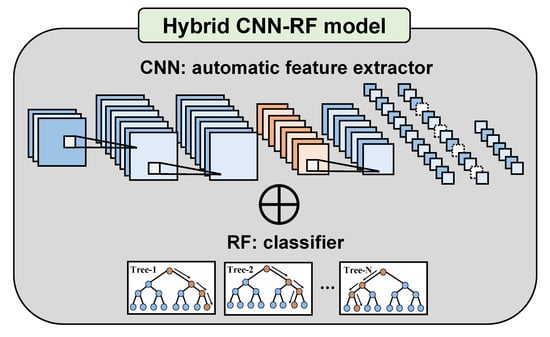
In the hybrid CNN-RF model, RF is applied to classify high-level features extracted from the CNN by considering the advantages of both CNN and RF. CNN-RF uses spatial features extracted from the optimal structure and parameters of the CNN as input for the classification. Therefore, no additional feature extraction or selection stages are required prior to the RF-based classification. Compared with the fully connected layer as a classifier in CNN, RF uses more sophisticated classification strategies, such as bagging [38]. Furthermore, the advantages of RF, including its robustness to outliers and its ability to reduce overfitting, can improve the classification performance, even when proper or informative spatial features cannot be extracted from CNN because of insufficient training data and input images.
3.2. Training and Reference Data Sampling
This study focused on investigating the applicability of CNN-RF in case where limited input data are used for early crop classification. To consider the case wherein limited training data are available in early crop mapping, the classification performance is compared and evaluated with respect to the different sizes of training data.
Both training datasets with different sizes and reference data were first extracted from the ground truth maps shown in Figure 1b and Figure 2b, which were subsequently used for classification and accuracy evaluation, respectively (Table 2). Five training data with different sizes were prepared to analyze the effect of training data size on the classification performance. Here, the ratio of the number of training pixels between classes was defined based on the size of crop fields within each study area. Randomly extracted 20,000 pixels that did not overlap the training pixels were used as reference data for both areas.
3.3. Optimization of Model Parameters
As the parameters of the ML and DL models greatly affect the classification accuracy, the determination of optical parameters is vital in achieving satisfactory classification accuracy and generalization capability. Detailed parameter information tested by the three classifiers is presented in Table 3.
Unlike other ML models such as SVM, RF requires relatively few parameters to be set, such as the number of trees to be grown in the forest (ntree) and the number of variables for the node partitioning (mtry) [16]. The optimal values of ntree and mtry were determined based on a grid search procedure for various parameter combinations.
In a CNN, several parameters, including the number of layers, image patch size, and number and size of convolution filters, must be carefully determined to obtain a satisfactory classification performance. The optimal structure of the CNN model depends heavily on both the parameters and inputs. In particular, the image patch size can significantly affect the classification performance [9,24,25,46]. Using a small patch size may result in overfitting of the model [43], whereas a large patch size may generate over-smoothed classification results [9]. In this study, eight different image patch sizes from 3 to 17, with an interval of 2, were first examined by considering the crop field scale within the study area. Based on our previous study [24], the size of the convolution filter was set to 3 × 3 to avoid the over-smoothing of the feature maps. Another important parameter is the depth of the network (the number of layers). The depth significantly affects the classification accuracy as the level or information content of the trained feature maps varies according to the number of layers [47]. Based on our DL-based classification results using UAV images [24,25], the number of layers was set to six to balance the complexity and robustness of the network structure. ReLU was applied as an activation function for all layers except for the last fully connected layer.
Two distinct regularization strategies were applied to prevent overfitting while training the CNN model. Dropout regularization, which randomly drops certain neurons during the training phase, was employed to reduce the inter-dependent learning among neurons. Early stopping was applied as the second regularization strategy to stop training at the specified number of iterations (epochs) when the model performance did not improve any further during the iterative training process. The Adam optimizer with a learning rate of 0.001 and cross entropy loss was applied to the model training as its effectiveness in time-series data classification has been proven previously [11,45].
The CNN-RF model shares the network structure of the CNN model, but some parameters must be adjusted prior to the RF-based classification. As features extracted from the fully connected layer are used as inputs for the RF classifier, mtry and ntree are determined using a grid search procedure similar to that in the RF model. Figure 4 shows the architecture of the CNN-RF model developed in this study.
Five-fold cross-validation was employed for optimal model training. Of the five partitions of training data, four were used for the model training. The remaining partition was used as validation samples to seek the optimal hyper-parameters of the classification models.
3.4. Incremental Classification
An incremental classification procedure [11,39] was employed to seek the optimal time-series set with fewer images for early crop mapping. Supervised classification is first conducted using RF, CNN, and CNN-RF classifiers using the initially acquired UAV images presented in Table 1 (A1 and H1 for Anbandegi and Hapcheon, respectively). Classification is then conducted incrementally using a time-series set in which the subsequent UAV image is progressively added to the images used for the previous classification. In the incremental classification, A8 and H3 in Table 1 indicate that eight and three images were used for classification in Anbandegi and Hapcheon, respectively. This procedure facilitates both the analysis of variations in the classification performance with respect to the growing cycles of crops, and the determination of the best classifier that effectively identifies crop types as early as possible.
3.5. Analysis Procedures and Implementation
The processing steps applied in this study for crop classification are shown in Figure 5. After preparing datasets for classification, temporal variations in the vegetation index (VI) for each crop type were first analyzed to identify the optimal dates for early crop mapping and obtain supporting information for the interpretation of results. The commonly used VI is the normalized difference in vegetation index (NDVI) based on reflectance values from the red and near-infrared spectral bands. However, it is not feasible to compute NDVI as the UAV system is not equipped with the near-infrared spectral sensor. Instead, the modified green-red vegetation index (MGRVI), which is a VI based on the visible bands [48], was computed in the study areas. The average MGRVI value per crop type was then computed using ground truth maps.
After the optimal hyper-parameters for CNN were selected using five-fold cross-validation, the spectral features and spatial features extracted by the CNN were then visualized using t-distributed stochastic neighbor embedding (t-SNE) for qualitative comparison of class separability. The t-SNE is a nonlinear dimensionality reduction technique of high-dimensional data for visualization in the 2D space [49,50]. This is employed to visually compare the relative differences in class separability in the feature space regarding the different training data and input images. All training samples in each class were projected onto the 2D using t-SNE.
All three classifiers with the optimized hyper-parameters were then applied to generate incremental classification results with respect to the different combination cases for training data sizes and the lengths of the time-series. The classification performance of the three different classifiers was quantitatively evaluated with respect to different training data sizes and the time-series length. After preparing a confusion matrix using independent reference data, the overall accuracy (OA) and F-measure were calculated and used as quantitative accuracy measures. The F-measure is defined as the harmonic mean of precision and recall, wherein the precision and recall correspond to the user’s accuracy and product’s accuracy, respectively [11]. As the DL models have a stochastic nature, considerably different classification results may be achieved even with the same input images and training data. To ensure a fair comparison of the classification performance of the three classifiers, the classification was repeated five times for each classifier. The average and standard deviation of the five accuracy values were used for the quantitative comparison. For each independent classification run, different training samples were randomly selected using different random seeds, but the total number of training data for the five different cases of training data in Table 2 was fixed. Based on the quantitative accuracy measures, time-series analysis of VI, and qualitative analysis results of class separability, the classification results were finally interpreted in the context of early crop mapping.
4. Results
4.1. Time-Series Analysis of Vegetation Index
Figure 6 shows the temporal variations in the average MGRVI for individual crop types in the two study areas. As shown in Figure 6a, June UAV images in Anbandegi provide useful information to distinguish the highland Kimchi cabbage from other crops because of the difference in the sowing time. As the difference in MGRVI between potato and cabbage increased from the end of June, the image in late June (A3) or mid-July (A4) is useful for distinguishing between potato and cabbage. The MGRVI value of fallow was consistently high throughout the entire crop growth cycle. Hence, it is relatively easy to discriminate fallow from crops. The time when the optimal OA is achieved for early crop mapping may vary annually depending on the agricultural environment; however, the optimal time in 2018 for early crop mapping in Anbandegi was at the end of June (A3) or middle of July (A4).
In Hapcheon, the MGRVI values of all the crops increased gradually from April to May, and only slight differences in the variation of MGRVI were observed, except for onion (Figure 6b). Consequently, it may be difficult to discern crops, even if all time-series images are used for the classification. In contrast, it is easy to identify fallow that is consistently managed as bare soil while crops are growing.
Such different behaviors of vegetation vitality in the two study areas imply the different effects of limited input images on the classification accuracy.
4.2. Comparison of Class Separability in the Feature Space
The final optimal hyper-parameters determined from 5-fold cross validation are given in Tables S1 and S2 for Anbandegi and Hapcheon, respectively.
Figure 7 and Figure 8 show the feature embedding of features using the combination of two differently sized training data (T1 vs. T5) and two different input images (first image vs. all images) for Anbandegi and Hapcheon, respectively. These representative cases were visualized for comparison purposes. The spectral features indicate three spectral bands of each UAV imagery.
In Anbandegi (Figure 7), the spatial features extracted from CNN are likely to better separate all crops than the spectral features. The spatial features extracted from CNN with all eight images (A8) and the largest number of training data (T5) maximize the interclass variability and minimize the intraclass variability, thereby clearly separating each crop type. When using all eight images (A8) and the smallest training data (T1), each crop type is better distinguished in the CNN-based feature space than in the spectral feature space. The CNN-based features show much better class separability than spectral features when using A1 and T1, particularly for highland Kimchi cabbage, which is the major crop type in Anbandegi. All crops are widely spread out and overlap significantly in the spectral feature space, whereas the highland Kimchi cabbage and fallow samples are well discretized in the CNN-based spatial feature space. However, cabbage and potato samples slightly overlap in the CNN-based feature space because of their similar sowing times, thus indicating that CNN-based features may not provide useful information for classification in the worst case of data availability.
In Hapcheon, as shown in Figure 8, better class separability was obtained in spatial features extracted from CNN than the spectral features, similar to the results in Anbandegi. For example, barley and garlic samples largely overlap in the spectral feature space, regardless of the training data size and the length of the time-series. As shown in the temporal profiles of MGRVI in Figure 6b, the small changes in MGRVI of barley and garlic samples during the entire growth period led to large overlaps in the spectral feature space. However, onion samples were well discretized owing to the gradual change in MGRVI, unlike other crops. It should be noted that in the case of T1, the difference in class separability between garlic and barley for H1 and H3 is insignificant, unlike in Anbandegi.
The visual comparison results of feature embedding in the two study areas indicate that the CNN-based spatial features are more useful for crop classification than the spectral features. However, some confusion still persists between some crop types in the CNN-based feature space when using the smallest training data (T1) and input images. This implies the necessity of applying a more sophisticated classifier.
4.3. Incremental Classification Results
4.3.1. Results in Anbandegi
Figure 9 shows the variations in average OA of the three different classifiers in Anbandegi with respect to five different training data sizes (T1 to T5) and eight different lengths of time-series (A1 to A8) used for classification. The standard deviation values of OA from five classification runs for different combination cases are presented in Table S3.
As expected, OA values for all classifiers increased as more input images and training data were used for classification. Using all eight images (A8) and the largest training data (T5) yielded the highest classification accuracy. In this case, both CNN and CNN-RF achieved a similar classification accuracy. For all combination cases, the best and worst classifiers were CNN-RF and RF, respectively. A substantial improvement in the OA of CNN-RF over RF and CNN was obtained when using only one image and two images (A1 and A2) with small training data (T1 and T2) for classification. The maximum increases in the OA of CNN-RF over RF and CNN are 21.3%p for A2 and T2 and 6.7%p for A1 and T2, respectively. Given a much larger number of reference samples (20,000) than the training samples (80 to 1280), the small difference in the OA between CNN-RF and CNN can be considered significant. When accuracy statistics are calculated using large reference samples, even small difference in the OA indicates that the number of correctly classified samples is large. Furthermore, the OA between CNN-RF and CNN for each classification run with respect to the combination cases with limited input data was statistically significant at the 5% significance level from the McNemar test [54].
When adding input images until the A3 case (the optimal date identified from Figure 6a), the greatest increase in OA was achieved for all classifiers, regardless of the training data size. Conversely, the incremental classification results using more input images (A4 to A8) yielded a slight increase in OA for T1 and T2, but a small change in OA for T3 to T5. Similar OA values for A3 and A4 indicate that the optimal time in 2018 for early crop mapping was the end of June (A3) as the fewest possible images are preferred for early crop mapping. When three images until the end of June (A3) were used with relatively small training samples (T2), the OA of CNN-RF was 14.4%p and 2.1%p higher than RF and CNN, respectively. In contrast, the cases using relatively large training samples (T4 and T5) yielded a similar classification accuracy between CNN and CNN-RF. Therefore, CNN-RF is more beneficial than CNN for early crop mapping in Anbandegi when using only a few images acquired until the optimal date and small training samples.
Figure 10 shows the F-measure for each crop type of specific incremental classification results generated using T1 (the case with a large difference in OA between classifiers) and T5 (the case with the highest OA for all classifiers). The largest difference in the OA was observed for T2. However, the incremental classification result for T1 was selected for the comparison as T1 yielded a similar temporal variation in OA and showed slightly higher distinctive class separability of CNN-based spatial features than the spectral features (Figure 7).
When using T1, the F-measure of highland Kimchi cabbage increased from A1 to A3 and showed slight variation from A4 to A8. This is consistent with the results of temporal variations in MGRVI suggesting that the optimal time for the classification of all crops in Anbandegi is the end of June (A3), as shown in Figure 6a. The best classifier of highland Kimchi cabbage is CNN-RF. The improvement in the F-measure of CNN-RF compared to RF and CNN is 18.5%p and 3.5%p for A1 and T1, respectively. The F-measure of cabbage and potato for the T1 increased significantly for all three classifiers from A1 to A4, except for the F-measure of potato for RF. Such an increase in the F-measure is mainly due to the increasing difference in MGRVI between cabbage and potato from the end of June (A3) to the middle of July (A4) (Figure 6a). Similar to highland Kimchi cabbage, the best classifier for cabbage and potato was also CNN-RF.
However, when a single image was used for classification (A1 with T1), the F-measure of CNN was lower than that of RF. As shown in Figure 7, both cabbage and potato samples are spread widely and overlap in both the spectral features and CNN-based spatial features. Meanwhile, despite similar or slightly more overlapping of those crops in the spectral feature space, RF showed better classification accuracy for potato and cabbage than CNN. This indicates that CNN-based spatial features cannot provide useful information to classify cabbage and potato for the worst case of data availability. Consequently, the poor classification performance of CNN is caused by both the failure to extract informative spatial features and the application of the fully connected layer as a classifier. Conversely, this result demonstrates a better classification capability of RF than CNN. By applying RF as a sophisticated classifier to the CNN-based spatial features, CNN-RF can distinguish between cabbage and potato more accurately than CNN and RF.
When using the largest training samples (T5), the F-measure values of all crops increased from A1 to A3 and varied slightly from A4 to A8. The highest F-measure values for all crops were achieved by CNN-RF when fewer images were used for classification (A3). The F-measure values of CNN and CNN-RF were very similar, as more images were used for the classification (A4 to A8).
The quantitative accuracy assessment results shown in Figure 9 and Figure 10 indicate that CNN-RF is the most accurate classifier for crop mapping in the study area, regardless of the training data size and length of the time-series. Furthermore, the superiority of CNN-RF over RF and CNN is more prominent for the worst data availability with limited training data and input images; this confirms the potential of CNN-RF for early crop mapping.
To illustrate the advantage of CNN-RF for early crop mapping, the specific classification results using T2 which showed significant differences in the OA between classifiers, are shown in Figure 11 for visual comparison. Highland Kimchi cabbage fields are properly classified when one image (A1) and three images (A3) are used with small training samples, except for certain isolated pixels at field boundaries. However, most cabbage and potato fields are misclassified when only one image (A1) is used as the input. As the sowing time of cabbage and potato is early June, using a single June image is not adequate for their discrimination. Conversely, adding more images acquired until the end of June (A1 to A3) substantially reduced the misclassified pixels in cabbage and potato fields. Although noise effects still exist, the overall classification result using A3 is similar to that using all eight images (A8), thus demonstrating the benefit of CNN-RF for early crop mapping.
4.3.2. Results in Hapcheon
The OA in Hapcheon increased for all classifiers as more input images and training samples were used for classification, similar to the results in Anbandegi (Figure 12). Average OA and standard deviation values from five classification runs are presented in Table S4. The maximum OA values for RF, CNN, and CNN-RF were 82.6%, 91.7%, and 92.1%, respectively, with CNN-RF achieving the highest OA when using all three images (H3) along with the largest training data (T5). Furthermore, even with limited inputs, CNN-RF was the best classifier in the study area, and the difference in the OA between CNN-RF and CNN for each classification run was statistically significant from the McNemar test.
Unlike Anbandegi, variations in the OA in Hapcheon were affected more by the training data size than the length of the time-series. The minor impact of the length of the time-series can be explained by the small number of input images and the slight difference observed in the temporal variation in MGRVI of the three images. When all three images (H3) were used for classification with CNN-RF, its OA for T5 increased by 13.1%p, compared with that for T1. However, for T5, the improvement in the OA of H3 over H1 was 4.9%p. In some cases, a slight decrease in OA was achieved for RF and CNN (RF with H3 and T2, and CNN with H2 and T2). Similar patterns in the feature space for H1 and H3 in Figure 8 yielded a slight improvement in the OA. Based on these results, early or middle April is estimated to be the optimal date in 2019 for early crop mapping in Hapcheon, when sufficient training samples are unavailable. The best classifier for early crop mapping is CNN-RF, similar to that in Anbandegi.
The variations in the class-wise F-measure for the two different training data sizes (T1 and T5) are shown in Figure 13. In the case of T1 (smallest training samples), the F-measure values for garlic and barley were lower than those for onion for all three classifiers. In particular, the F-measure of barley for RF and CNN was very low when using H1. Using more images did not improve the accuracy of barley. The low accuracy for garlic and barely is mainly due to the spectral similarity in Figure 6b and the low class separability in Figure 8. The F-measure of barley for CNN-RF was not high (0.68) in the case of T1, but CNN-RF increased the F-measure by approximately 9.6%p, compared with that for CNN. Furthermore, CNN-RF increased the F-measure for garlic when all three images were used. The accuracy of onion and fallow for H3 was lower than that for H2 because of the confusion between the two crops (1.9%p and 2.6%p lower for onion and fallow, respectively), but the OA of CNN-RF was still 4.2%p higher than that of CNN (Figure 12).
In the case of T5 (the largest training samples), a small variation in accuracy for onion and fallow was observed for all three classifiers. The class-wise accuracy values of CNN-RF are similar to those of CNN, regardless of the number of input images. The F-measure of barley was improved by approximately 10%p for all three classifiers.
As the classification accuracy is less affected by the length of the time-series, collecting sufficient training samples is vital for early crop mapping in Hapcheon. When considering the difficulty in collecting sufficient training samples, CNN-RF is the best classifier for the early stage classification of crops with high similarity using limited training samples.
Figure 14 shows the incremental classification results of CNN-RF with T1 for different input images. Considering the difficulty in collecting training samples, T1 (the smallest training samples) was selected for the visual comparison. The confusion between garlic and barley is observed for all classification results. When using only one image (H1), the misclassification of barley occurs more in the classification result; however, other crops are well identified, compared with the classification results using more images. As the major crop types in the study area are onion and garlic, it can be concluded that CNN-RF can generate reliable classification results in Hapcheon even with limited inputs for early crop mapping (T1 and H1).
5. Discussion
Unlike most previous studies on early crop mapping focusing on the effects of various time-series image combinations for the selection of optimal dates [10,11,55,56], the main contribution of this study is the assessment of the classification accuracy considering the data availability conditions specific to early crop mapping. These include the training sample sizes and the length of the time-series, along with the benefit of CNN-RF as a sophisticated classifier for the same body of work.
From a methodological viewpoint, CNN-RF is attractive for supervised classification. Using informative high-level spatial features extracted from CNN is more promising than using only spectral information. Thus, end-to-end learning, automatic extraction of such spatial features that can account for spatial contextual information, is the merit of CNN. However, a large amount of training data is usually required to extract informative high-level spatial features in CNN-based classification [37]. The CNN models trained using limited training data may produce poor classification accuracy. Moreover, in the worst case of data availability, a simple classifier such as the full connected layer with a softmax activation function in the CNN model may fail to achieve satisfactory classification performance. In this case, more sophisticated conventional ML classifiers can be applied to the incomplete spatial features extracted by the CNN. Once input features are prepared for classification, RF is one of the promising ML classifiers as it applies more sophisticated classification strategies to avoid overfitting. However, much effort is required for the preparation of input features prior to the RF-based classification. The strength of CNN-RF is its ability to combine the complementary characteristics of CNN (a simple classifier with an automatic spatial feature extractor) and RF (a sophisticated classifier without a feature extractor). As RF requires fewer user-defined parameters, CNN-RF enables end-to-end learning with a satisfactory classification performance. Therefore, CNN-RF is a promising classifier for supervised classification using limited training data, particularly for early crop mapping.
Despite the promising results of CNN-RF for early crop mapping, some aspects can be improved through future research. With CNN-RF, once the optimal time for early crop mapping has been determined, the number of training samples is critical to achieve satisfactory classification accuracy [56]. In this study, using more training samples with images acquired until the optimal date yielded higher classification accuracy (Figure 9 and Figure 12). Thus, developing strategies to add informative samples to the training data is necessary. The first possible strategy is data augmentation (DA), which artificially increases the quantity of training data [10,57]. However, if DA is applied to the training data collected during the early growth stage, wherein confusion between crops may exist, the classification accuracy may not significantly improve as ambiguous samples with questionable labels are likely to be selected. Another possible strategy is to select informative unlabeled pixels through the learning process and subsequently add them to the training data. Semi-supervised learning [58], active learning [59] or self-learning [18] can be applied to extract informative pixels as candidates for new training data. CNN-RF can be employed as a basic module for the feature extraction and classification within an iterative framework. However, the iterative addition of new informative pixels incurs high computational costs, particularly in DL-based classification. It should be noted that whatever strategy is applied to expand the training data, the focus should be on increasing the diversity of training data to improve the generalization ability of the classification model.
In this study, a feature selection procedure was not employed because few features are available for early crop mapping with limited input data. As not all CNN-based spatial features contribute equally to the identification of different crop types, assigning more weights to informative features can improve the classification performance. Within the CNN-RF framework, the weighting scheme such as squeeze-and-excitation networks [60] can be combined to assign feature-specific weights to CNN-based spatial features. The weighted CNN-based spatial features are then fed into the RF classifier. Another possible approach is a metric learning network in which the similarity between high-dimensional features is evaluated during training the CNN model [61]. Thus, it is worthwhile to investigate the potential of the improved feature learning scheme in future work.
In this study, ultra-high spatial resolution UAV images were used as inputs for the crop classification as most crops in Korea are usually cultivated in small fields. If remote sensing images with coarser spatial resolutions are used for early crop mapping, the mixed pixel effects of training samples are inevitable and may greatly affect the classification performance as they may fail to provide the representative signature of individual crops. Recently, Park and Park [62] reported that the classification performance of CNN-based classification depends on the class purity within a training patch. Thus, this aspect should be considered in future studies on satellite images with coarser spatial resolutions than UAV images to generalize the key findings of this study.
6. Conclusions
The provision of early information on the crop types and distributions is critical for the timely evaluation of crop yield and production for food security. This study quantitatively evaluated the potential of the hybrid classification model (CNN-RF) that leverages the advantages of both CNN and RF to improve the classification performance for early crop mapping. Crop classification experiments using UAV images in the two study areas in Korea demonstrated the benefits of CNN-RF for early crop mapping. The superiority of CNN-RF over CNN and RF is prominent when fewer images and smaller training samples are used for classification. Fewer image times-series are preferred for early crop mapping and collecting sufficient training samples is often difficult during the early growth stage of crops. This case wherein limited input datasets are available is common in supervised classification due to cloud contamination of optical images and the difficulty in collecting sufficient training samples. Therefore, the hybrid CNN-RF classifier presented in this study is expected to be a promising classifier for general supervised classification tasks using limited input data as well as early crop mapping. Furthermore, the optimal time for early crop mapping determined in this study can be effectively used to plan future UAV image acquisitions in the study area.
Supplementary Materials
The following are available online at https://www.mdpi.com/article/10.3390/rs13091629/s1, Table S1: Optimal hyper-parameter values determined for combination cases of different training data sizes and the lengths of time-series in Anbandegi ( is the number of input variables). Table S2: Optimal hyper-parameter values determined for combination cases of different training data sizes and the lengths of time-series in Hapcheon ( is the number of input variables). Table S3: Average overall accuracy with standard deviation of five classification results with respect to combination cases of different training data sizes and the lengths of time-series in Anbandegi (the best case is shown in bold. Table S4: Average overall accuracy with standard deviation of five classification results with respect to combination cases of different training data sizes and the lengths of time-series in Hapcheon (the best case is shown in bold).
Author Contributions
Conceptualization, G.-H.K., N.-W.P., C.-w.P., K.-d.L., S.-i.N., and H.-y.A.; methodology, G.-H.K. and N.-W.P.; formal analysis, G.-H.K.; data curation, C.-w.P., K.-d.L., S.-i.N., and H.-y.A.; writing—original draft preparation, G.-H.K. and N.-W.P.; writing—review and editing, C.-w.P., K.-d.L., S.-i.N., and H.-y.A.; supervision, N.-W.P. All authors have read and agreed to the published version of the manuscript.
Funding
This study was carried out with the support of “Cooperative Research Program for Agriculture Science & Technology Development (Project No. PJ01350004)” Rural Development Administration, Korea.
Data Availability Statement
Data sharing is not applicable to this manuscript.
Acknowledgments
The authors thank the anonymous reviewers for their constructive comments on the manuscript.
Conflicts of Interest
The authors declare no conflict of interest.
References
- Weiss, M.; Jacob, F.; Duveiller, G. Remote sensing for agricultural applications: A meta-review. Remote Sens. Environ. 2020, 236, 111402. [Google Scholar] [CrossRef]
- Kim, N.; Ha, K.J.; Park, N.W.; Cho, J.; Hong, S.; Lee, Y.W. A comparison between major artificial intelligence models for crop yield prediction: Case study of the Midwestern United States, 2006–2105. ISPRS Int. J. Geo-Inf. 2019, 8, 240. [Google Scholar] [CrossRef] [Green Version]
- Na, S.I.; Park, C.W.; So, K.H.; Ahn, H.Y.; Lee, K.D. Application method of unmanned aerial vehicle for crop monitoring in Korea. Korean J. Remote Sens. 2018, 34, 829–846, (In Korean with English Abstract). [Google Scholar] [CrossRef]
- Kwak, G.H.; Park, N.W. Impact of texture information on crop classification with machine learning and UAV images. Appl. Sci. 2019, 9, 643. [Google Scholar] [CrossRef] [Green Version]
- Immitzer, M.; Vuolo, F.; Atzberger, C. First experience with Sentinel-2 data for crop and tree species classifications in central Europe. Remote Sens. 2016, 8, 166. [Google Scholar] [CrossRef]
- Böhler, J.E.; Schaepman, M.E.; Kneubühler, M. Crop classification in a heterogeneous arable landscape using uncalibrated UAV data. Remote Sens. 2018, 10, 1282. [Google Scholar] [CrossRef] [Green Version]
- Villa, P.; Stroppiana, D.; Fontanelli, G.; Azar, R.; Brivio, P.A. In-season mapping of crop type with optical and X-band SAR data: A classification tree approach using synoptic seasonal features. Remote Sens. 2015, 7, 12859–12886. [Google Scholar] [CrossRef] [Green Version]
- Hao, P.; Zhan, Y.; Wang, L.; Niu, Z.; Shakir, M. Feature selection of time series MODIS data for early crop classification using random forest: A case study in Kansas, USA. Remote Sens. 2015, 7, 5347–5369. [Google Scholar] [CrossRef] [Green Version]
- Ji, S.; Zhang, C.; Xu, A.; Shi, Y.; Duan, Y. 3D convolutional neural networks for crop classification with multi-temporal remote sensing images. Remote Sens. 2018, 10, 75. [Google Scholar] [CrossRef] [Green Version]
- Wei, S.; Zhang, H.; Wang, C.; Wang, Y.; Xu, L. Multi-temporal SAR data large-scale crop mapping based on U-Net model. Remote Sens. 2019, 11, 68. [Google Scholar] [CrossRef] [Green Version]
- Zhao, H.; Chen, Z.; Jiang, H.; Jing, W.; Sun, L.; Feng, M. Evaluation of three deep learning models for early crop classification using Sentinel-1A imagery time series—A case study in Zhanjiang, China. Remote Sens. 2019, 11, 2673. [Google Scholar] [CrossRef] [Green Version]
- Skakun, S.; Franch, B.; Vermote, E.; Roger, J.C.; Becker-Reshef, I.; Justice, C.; Kussul, N. Early season large-area winter crop mapping using MODIS NDVI data, growing degree days information and a Gaussian mixture model. Remote Sens. Environ. 2017, 195, 244–258. [Google Scholar] [CrossRef]
- Foody, G.M.; Mathur, A. The use of small training sets containing mixed pixels for accurate hard image classification: Training on mixed spectral responses for classification by a SVM. Remote Sens. Environ. 2006, 103, 179–189. [Google Scholar] [CrossRef]
- Deng, F.; Pu, S.; Chen, X.; Shi, Y.; Yuan, T.; Pu, S. Hyperspectral image classification with capsule network using limited training samples. Sensors 2018, 18, 3153. [Google Scholar] [CrossRef] [Green Version]
- Mas, J.F.; Flores, J.J. The application of artificial neural networks to the analysis of remotely sensed data. Int. J. Remote Sens. 2008, 29, 617–663. [Google Scholar] [CrossRef]
- Tatsumi, K.; Yamashiki, Y.; Morante, A.K.; Fernández, L.R.; Nalvarte, R.A. Pixel-based crop classification in Peru from Landsat 7 ETM+ images using a random forest model. J. Agric. Meteorol. 2016, 72, 1–11. [Google Scholar] [CrossRef] [Green Version]
- Ma, L.; Fu, T.; Blaschke, T.; Li, M.; Tiede, D.; Zhou, Z.; Ma, X.; Chen, D. Evaluation of feature selection methods for object-based land cover mapping of unmanned aerial vehicle imagery using random forest and support vector machine classifiers. ISPRS Int. J. Geo-Inf. 2017, 6, 51. [Google Scholar] [CrossRef]
- Kim, Y.; Park, N.W.; Lee, K.D. Self-learning based land-cover classification using sequential class patterns from past land-cover maps. Remote Sens. 2017, 9, 921. [Google Scholar] [CrossRef] [Green Version]
- Löw, F.; Michel, U.; Dech, S.; Conrad, C. Impact of feature selection on the accuracy and spatial uncertainty of per-field crop classification using support vector machines. ISPRS J. Photogramm. Remote Sens. 2013, 85, 102–119. [Google Scholar] [CrossRef]
- Sidike, P.; Sagan, V.; Maimaitijiang, M.; Maimaitiyiming, M.; Shakoor, N.; Burken, J.; Mockler, T.; Fritschi, F.B. dPEN: Deep Progressively Expanded Network for mapping heterogeneous agricultural landscape using WorldView-3 satellite imagery. Remote Sens. Environ. 2019, 221, 756–772. [Google Scholar] [CrossRef]
- Zhao, W.; Du, S. Spectral–spatial feature extraction for hyperspectral image classification: A dimension reduction and deep learning approach. IEEE Trans. Geosci. Remote Sens. 2016, 54, 4544–4554. [Google Scholar] [CrossRef]
- Yang, X.; Ye, Y.; Li, X.; Lau, R.Y.; Zhang, X.; Huang, X. Hyperspectral image classification with deep learning models. IEEE Trans. Geosci. Remote Sens. 2018, 56, 5408–5423. [Google Scholar] [CrossRef]
- Song, H.; Kim, Y.; Kim, Y. A patch-based light convolutional neural network for land-cover mapping using Landsat-8 images. Remote Sens. 2019, 11, 114. [Google Scholar] [CrossRef] [Green Version]
- Kwak, G.H.; Park, C.W.; Lee, K.D.; Na, S.I.; Ahn, H.Y.; Park, N.W. Combining 2D CNN and bidirectional LSTM to consider spatio-temporal features in crop classification. Korean J. Remote Sens. 2019, 35, 681–692, (In Korean with English Abstract). [Google Scholar] [CrossRef]
- Park, M.G.; Kwak, G.H.; Park, N.W. A convolutional neural network model with weighted combination of multi-scale spatial features for crop classification. Korean J. Remote Sens. 2019, 35, 1273–1283, (In Korean with English Abstract). [Google Scholar] [CrossRef]
- Chen, X.; Xiang, S.; Liu, C.L.; Pan, C.H. Vehicle detection in satellite images by hybrid deep convolutional neural networks. IEEE Geosci. Remote Sens. Lett. 2014, 11, 1797–1801. [Google Scholar] [CrossRef]
- Li, K.; Cheng, G.; Bu, S.; You, X. Rotation-insensitive and context-augmented object detection in remote sensing images. IEEE Trans. Geosci. Remote Sens. 2018, 56, 2337–2348. [Google Scholar] [CrossRef]
- Zhu, X.X.; Tuia, D.; Mou, L.; Xia, G.S.; Zhang, L.; Xu, F.; Fraundorfer, F. Deep learning in remote sensing: A comprehensive review and list of resources. IEEE Geosci. Remote Sens. Mag. 2017, 5, 8–36. [Google Scholar] [CrossRef] [Green Version]
- Zhong, L.; Hu, L.; Zhou, H. Deep learning based multi-temporal crop classification. Remote Sens. Environ. 2019, 221, 430–443. [Google Scholar] [CrossRef]
- Crisóstomo de Castro Filho, H.; Abílio de Carvalho Júnior, O.; Ferreira de Carvalho, O.L.; Pozzobon de Bem, P.; dos Santos de Moura, R.; Olino de Albuquerque, A.; Rosa Silva, C.; Guimaraes Ferreira, P.H.; Fontes Guimaraes, R.; Trancoso Gomes, R.A. Rice crop detection using LSTM, Bi-LSTM, and machine learning models from sentinel-1 time series. Remote Sens. 2020, 12, 2655. [Google Scholar] [CrossRef]
- Kussul, N.; Lavreniuk, M.; Skakun, S.; Shelestov, A. Deep learning classification of land cover and crop types using remote sensing data. IEEE Geosci. Remote Sens. Lett. 2017, 14, 778–782. [Google Scholar] [CrossRef]
- Xie, B.; Zhang, H.K.; Xue, J. Deep convolutional neural network for mapping smallholder agriculture using high spatial resolution satellite image. Sensors 2019, 19, 2398. [Google Scholar] [CrossRef] [Green Version]
- Kim, Y.; Kwak, G.H.; Lee, K.D.; Na, S.I.; Park, C.W.; Park, N.W. Performance evaluation of machine learning and deep learning algorithms in crop classification: Impact of hyper-parameters and training sample size. Korean J. Remote Sens. 2018, 34, 811–827, (In Korean with English Abstract). [Google Scholar] [CrossRef]
- Du, P.; Xia, J.; Zhang, W.; Tan, K.; Liu, Y.; Liu, S. Multiple classifier system for remote sensing image classification: A review. Sensors 2012, 12, 4764–4792. [Google Scholar] [CrossRef] [PubMed]
- Yang, S.; Gu, L.; Li, X.; Jiang, T.; Ren, R. Crop classification method based on optimal feature selection and hybrid CNN-RF networks for multi-temporal remote sensing imagery. Remote Sens. 2020, 12, 3119. [Google Scholar] [CrossRef]
- Wang, A.; Wang, Y.; Chen, Y. Hyperspectral image classification based on convolutional neural network and random forest. Remote Sens. Lett. 2019, 10, 1086–1094. [Google Scholar] [CrossRef]
- Dong, L.; Du, H.; Mao, F.; Han, N.; Li, X.; Zhou, G.; Zhu, D.; Zheng, J.; Zhang, M.; Xing, L.; et al. Very high resolution remote sensing imagery classification using a fusion of random forest and deep learning technique—Subtropical area for example. IEEE J. Sel. Top. Appl. Earth Obs. Remote Sens. 2020, 13, 113–128. [Google Scholar] [CrossRef]
- Li, T.; Leng, J.; Kong, L.; Guo, S.; Bai, G.; Wang, K. DCNR: Deep cube CNN with random forest for hyperspectral image classification. Multimed. Tools Appl. 2019, 78, 3411–3433. [Google Scholar] [CrossRef]
- Inglada, J.; Vincent, A.; Arias, M.; Marais-Sicre, C. Improved early crop type identification by joint use of high temporal resolution SAR and optical image time series. Remote Sens. 2016, 8, 362. [Google Scholar] [CrossRef] [Green Version]
- Yoo, H.Y.; Lee, K.D.; Na, S.I.; Park, C.W.; Park, N.W. Field crop classification using multi-temporal high-resolution satellite imagery: A case study on garlic/onion field. Korean J. Remote Sens. 2017, 33, 621–630, (In Korean with English Abstract). [Google Scholar] [CrossRef]
- Environmental Geographic Information Service (EGIS). Available online: http://egis.me.go.kr (accessed on 9 January 2021).
- Breiman, L. Random forests. Mach. Learn. 2001, 45, 5–32. [Google Scholar] [CrossRef] [Green Version]
- Guidici, D.; Clark, M.L. One-Dimensional convolutional neural network land-cover classification of multi-seasonal hyperspectral imagery in the San Francisco Bay Area, California. Remote Sens. 2017, 9, 629. [Google Scholar] [CrossRef] [Green Version]
- LeCun, Y.; Bengio, Y.; Hinton, G. Deep learning. Nature 2015, 521, 436–444. [Google Scholar] [CrossRef]
- Yoo, C.; Lee, Y.; Cho, D.; Im, J.; Han, D. Improving local climate zone classification using incomplete building data and Sentinel 2 images based on convolutional neural networks. Remote Sens. 2020, 12, 3552. [Google Scholar] [CrossRef]
- Feng, Q.; Zhu, D.; Yang, J.; Li, B. Multisource hyperspectral and LiDAR data fusion for urban land-use mapping based on a modified two-branch convolutional neural network. ISPRS Int. J. Geo-Inf. 2019, 8, 28. [Google Scholar] [CrossRef] [Green Version]
- Chen, S.; Wang, H.; Xu, F.; Jin, Y.Q. Target classification using the deep convolutional networks for SAR images. IEEE Trans. Geosci. Remote Sens. 2016, 54, 4806–4817. [Google Scholar] [CrossRef]
- Bendig, J.; Yu, K.; Aasen, H.; Bolten, A.; Bennertz, S.; Broscheit, J.; Gnyp, M.L.; Bareth, G. Combining UAV-based plant height from crop surface models, visible, and near infrared vegetation indices for biomass monitoring in barley. Int. J. Appl. Earth Obs. Geoinf. 2015, 39, 79–87. [Google Scholar] [CrossRef]
- Van der Maaten, L.; Hinton, G. Visualizing data using t-SNE. J. Mach. Learn. Res. 2008, 9, 2579–2605. [Google Scholar]
- Jiao, L.; Liang, M.; Chen, H.; Yang, S.; Liu, H.; Cao, X. Deep fully convolutional network-based spatial distribution prediction for hyperspectral image classification. IEEE Trans. Geosci. Remote Sens. 2017, 55, 5585–5599. [Google Scholar] [CrossRef]
- Scikit-Learn: Machine Learning in Python. Available online: https://scikit-learn.org (accessed on 9 January 2021).
- TensorFlow. Available online: https://tensorflow.org (accessed on 9 January 2021).
- Keras Documentation. Available online: https://keras.io (accessed on 9 January 2021).
- Foody, G.M. Thematic map comparison: Evaluating the statistical significance of differences in classification accuracy. Photogramm. Eng. Remote Sens. 2004, 70, 627–633. [Google Scholar] [CrossRef]
- Yi, Z.; Jia, L.; Chen, Q. Crop classification using multi-temporal Sentinel-2 data in the Shiyang River Basin of China. Remote Sens. 2020, 12, 4052. [Google Scholar] [CrossRef]
- Ren, T.; Liu, Z.; Zhang, L.; Liu, D.; Xi, X.; Kang, Y.; Zhao, Y.; Zhang, C.; Li, S.; Zhang, X. Early identification of seed maize and common maize production fields using Sentinel-2 images. Remote Sens. 2020, 12, 2140. [Google Scholar] [CrossRef]
- Li, W.; Chen, C.; Zhang, M.; Li, H.; Du, Q. Data augmentation for hyperspectral image classification with deep CNN. IEEE Geosci. Remote Sens. Lett. 2018, 16, 593–597. [Google Scholar] [CrossRef]
- Zhu, X. Semi-Supervised Learning Literature Survey; Technical Report 1530; Department of Computer Sciences, University of Wisconsin: Madison, WI, USA, 2005. [Google Scholar]
- Settles, B. Active Learning Literature Survey; Technical Report 1648; Department of Computer Sciences, University of Wisconsin: Madison, WI, USA, 2010. [Google Scholar]
- Hu, J.; Shen, L.; Sun, G. Squeeze-And-Excitation Networks. In Proceedings of the 2018 IEEE Conference on Computer Vision and Pattern Recognition (CVPR), Salt Lake City, UT, USA, 18–22 June 2018; pp. 7132–7141. [Google Scholar]
- Shi, C.; Lv, Z.; Shen, H.; Fang, L.; You, Z. Improved metric learning with the CNN for very-high-resolution remote sensing image classification. IEEE J. Sel. Top. Appl. Earth Obs. Remote Sens. 2021, 14, 631–644. [Google Scholar] [CrossRef]
- Park, S.; Park, N.W. Effects of class purity of training patch on classification performance of crop classification with convolutional neural network. Appl. Sci. 2020, 10, 3773. [Google Scholar] [CrossRef]
Figure 1.
First case study area for crop classification (Anbandegi): (a) UAV imagery on 15 August 2018; (b) ground truth map; (c) zoomed-in images of individual crops.
Figure 1.
First case study area for crop classification (Anbandegi): (a) UAV imagery on 15 August 2018; (b) ground truth map; (c) zoomed-in images of individual crops.


Figure 2.
Second case study area for crop classification (Hapcheon): (a) UAV imagery on 2 May 2019; (b) ground truth map; (c) zoomed-in images of individual crops.
Figure 2.
Second case study area for crop classification (Hapcheon): (a) UAV imagery on 2 May 2019; (b) ground truth map; (c) zoomed-in images of individual crops.

Figure 3.
Phenological calendar of different crops in the two study areas: (a) Anbandegi; (b) Hapcheon.
Figure 3.
Phenological calendar of different crops in the two study areas: (a) Anbandegi; (b) Hapcheon.

Figure 4.
Architecture of the hybrid CNN-RF model applied in this study (Conv: convolutional layer, MaxPool: max pooling layer, and FC: fully connected layer).
Figure 4.
Architecture of the hybrid CNN-RF model applied in this study (Conv: convolutional layer, MaxPool: max pooling layer, and FC: fully connected layer).

Figure 5.
Schematic diagram of the processing flow applied in this study.

Figure 6.
Temporal profiles of the average MGRVI values for the two study areas: (a) Anbandegi; (b) Hapcheon.
Figure 6.
Temporal profiles of the average MGRVI values for the two study areas: (a) Anbandegi; (b) Hapcheon.

Figure 7.
Feature embedding visualizations in Anbandegi: spectral features (first row) and CNN-based spatial features (second row) generated using A1 with T1 (first column), A1 with T5 (second column), all eight images with T1 (third column), and A8 with T5 (fourth column). Each point represents a training pixel per crop class.

Figure 8.
Feature embedding visualizations in Hapcheon: spectral features (first row) and CNN-based spatial features (second row) generated using H1 with T1 (first column), H1 with T5 (second column), all three images with T1 (third column), and all three images with T5 (fourth column). Each point represents a training pixel per crop class.

Figure 9.
Temporal variations in the OA of incremental classification results using five different training data sets for three classifiers in Anbandegi.
Figure 9.
Temporal variations in the OA of incremental classification results using five different training data sets for three classifiers in Anbandegi.

Figure 10.
Temporal variations in the F-measure for each crop in the incremental classification results using T1 (first row) and T5 (second row) for the three classifiers in Anbandegi.
Figure 10.
Temporal variations in the F-measure for each crop in the incremental classification results using T1 (first row) and T5 (second row) for the three classifiers in Anbandegi.

Figure 11.
Incremental classification maps by CNN-RF with T2 and different input images (A1, A3, and A8) in Anbandegi.
Figure 11.
Incremental classification maps by CNN-RF with T2 and different input images (A1, A3, and A8) in Anbandegi.

Figure 12.
Temporal variations in the OA of incremental classification results using five different training data sets for three classifiers in Hapcheon.
Figure 12.
Temporal variations in the OA of incremental classification results using five different training data sets for three classifiers in Hapcheon.

Figure 13.
Temporal variations in the F-measure for each crop in the incremental classification results using T1 (first row) and T5 (second row) for three classifiers in Hapcheon.
Figure 13.
Temporal variations in the F-measure for each crop in the incremental classification results using T1 (first row) and T5 (second row) for three classifiers in Hapcheon.

Figure 14.
Incremental classification maps by CNN-RF with T1 and different input images (H1, H2, and H3) in Hapcheon.
Figure 14.
Incremental classification maps by CNN-RF with T1 and different input images (H1, H2, and H3) in Hapcheon.


Table 1.
List of UAV images used for the crop classification in the two study areas.
| Area | Acquisition Date | Image Size | |
|---|---|---|---|
| Anbandegi | 7 June 2018 | (A1) | 1314 × 1638 |
| 16 June 2018 | (A2) | ||
| 28 June 2018 | (A3) | ||
| 16 July 2018 | (A4) | ||
| 1 August 2018 | (A5) | ||
| 15 August 2018 | (A6) | ||
| 4 September 2018 | (A7) | ||
| 19 September 2018 | (A8) | ||
| Hapcheon | 4 April 2019 | (H1) | 1866 × 1717 |
| 18 April 2019 | (H2) | ||
| 2 May 2019 | (H3) | ||
Table 2.
Number of training and reference pixels for each class in both study areas.
| Study Area | Class | Training Data Size | Reference Data | ||||
|---|---|---|---|---|---|---|---|
| T1 | T2 | T3 | T4 | T5 | |||
| Anbandegi | Highland Kimchi cabbage | 38 | 76 | 152 | 304 | 608 | 5000 |
| Cabbage | 19 | 38 | 76 | 152 | 304 | 5000 | |
| Potato | 10 | 20 | 40 | 80 | 160 | 5000 | |
| Fallow | 13 | 26 | 52 | 104 | 208 | 5000 | |
| Total | 80 | 160 | 320 | 640 | 1280 | 20,000 | |
| Hapcheon | Garlic | 33 | 66 | 132 | 264 | 528 | 5000 |
| Onion | 32 | 64 | 128 | 256 | 512 | 5000 | |
| Barley | 7 | 14 | 28 | 56 | 112 | 5000 | |
| Fallow | 8 | 16 | 32 | 64 | 128 | 5000 | |
| Total | 80 | 160 | 320 | 640 | 1280 | 20,000 | |
Table 3.
Hyper-parameters of the three models applied in this study ( is the number of input variables).
Table 3.
Hyper-parameters of the three models applied in this study ( is the number of input variables).
| Model | Hyper-Parameter (Layer Description) | Tested Hyper-Parameters |
|---|---|---|
| CNN and CNN-RF | Image patch size | 3 to 17 (interval of 2) |
| Convolution layer 1 | 32, 64, 128, 256 | |
| Convolution layer 2 | ||
| Convolution layer 3 | ||
| Dropout | 0.3, 0.5, 0.7 | |
| Model epochs | 1 to 500 (interval of 1) | |
| Learning rate | 0.0001, 0.0005, 0.001, 0.005 | |
| RF and CNN-RF | The number of trees to be grown in the forest (ntree) | 100, 500, 1000, 1500 |
| The number of variables for node partitioning (mtry) | , , |
Publisher’s Note: MDPI stays neutral with regard to jurisdictional claims in published maps and institutional affiliations. |
© 2021 by the authors. Licensee MDPI, Basel, Switzerland. This article is an open access article distributed under the terms and conditions of the Creative Commons Attribution (CC BY) license (https://creativecommons.org/licenses/by/4.0/).
Share and Cite
MDPI and ACS Style
Kwak, G.-H.; Park, C.-w.; Lee, K.-d.; Na, S.-i.; Ahn, H.-y.; Park, N.-W. Potential of Hybrid CNN-RF Model for Early Crop Mapping with Limited Input Data. Remote Sens. 2021, 13, 1629. https://doi.org/10.3390/rs13091629
AMA Style
Kwak G-H, Park C-w, Lee K-d, Na S-i, Ahn H-y, Park N-W. Potential of Hybrid CNN-RF Model for Early Crop Mapping with Limited Input Data. Remote Sensing. 2021; 13(9):1629. https://doi.org/10.3390/rs13091629
Chicago/Turabian StyleKwak, Geun-Ho, Chan-won Park, Kyung-do Lee, Sang-il Na, Ho-yong Ahn, and No-Wook Park. 2021. "Potential of Hybrid CNN-RF Model for Early Crop Mapping with Limited Input Data" Remote Sensing 13, no. 9: 1629. https://doi.org/10.3390/rs13091629
Note that from the first issue of 2016, this journal uses article numbers instead of page numbers. See further details here.