
Two Severe Prolonged Hydrological Droughts Analysis over Mainland Australia Using GRACE Satellite Data


1
College of Survey and Geo-Informatics, Tongji University, Shanghai 200092, China
2
College of Geodesy and Geomatics, Shandong University of Science and Technology, Qingdao 266590, China
*
Author to whom correspondence should be addressed.
Remote Sens. 2021, 13(8), 1432; https://doi.org/10.3390/rs13081432
Submission received: 22 February 2021
/
Revised: 3 April 2021
/
Accepted: 6 April 2021
/
Published: 8 April 2021
(This article belongs to the Section Environmental Remote Sensing)
Abstract
:In recent years, many droughts have happened over mainland Australia, especially the two severe prolonged droughts, from 2006 to 2009 and 2018 to 2020, resulting in serious water scarcity. Therefore, using the Total Storage Deficit Index (TSDI) from the Gravity Recovery and Climate Experiment (GRACE), we analyzed the two severe prolonged droughts from the perspective of the affected area, spatial evolution, frequency, severity and drought driving factors. The results show that the affected area of Drought 2006–2009 ranged from 57% to 95%, and that of Drought 2018–2020 ranged from 45% to 95%. Drought 2006–2009 took its rise in southeastern Australia and gradually spread to the central part. Drought 2018–2020 originated in the southwest corner of the Northern Territory and northern New South Wales, and gradually expanded to Western Australia and the whole New South Wales respectively. During Drought 2006–2009, Victoria suffered drought all months, including 59% mild drought and 41% moderate drought, North Territory had the highest drought severity of 44.26 and Victoria ranked the second high with the severity of 35.51 (cm months). For Drought 2018–2020, Northern Territory was also dominated by drought all months, including 92% mild drought and 8% moderate drought, the drought severities were in North Territory and Western Australia with 52.19 and 31.44 (cm months), respectively. Finally, the correlation coefficients between the two droughts and Indo-Pacific climate variability including El Niño-Southern Oscillation and Indian Ocean Dipole (IOD) are computed. By comparing the correlation coefficients of Drought 2018–2020 with Drought 2006–2009, we find that the impact of the El Niño on the hydrological drought becomes weaker while IOD is stronger, and the role of Southern Oscillation on droughts is diverse with the quite different spatial patterns. The results from Fourier analysis confirm that the two hydrological droughts are all related to Indo-Pacific climate variability but with slightly different driving mechanisms.

1. Introduction
Drought will potentially cause drastic consequences for global water resources management [1] agriculture production [2], ecological protection [3], as well as economic and social development [4]. Detecting and understanding the characteristics of the previous droughts are the preconditions to predict drought and of great importance for water resource management [5]. In recent decades, the high vulnerability and sensitivity to climate change have made Australia become a hotspot [6]. The Australia Millennium Drought from the mid-1990s to 2009, also known as the Big Dry, was the most severe in the historical record, especially for the two severe prolonged hydrological droughts (during 2006–2009 and 2017–2019) [7,8,9]. Therefore, it is meaningful to determine the drought driving factors and assess the affected area, spatial evolution, frequency and severity of the two prolonged droughts.
The traditional methods of drought monitoring are based on accurate precipitation and evapotranspiration observations on the ground stations, and these observations are limited to near-surface or groundwater zones [10]. Remote sensing techniques can provide unprecedented spatiotemporal resolution and accuracy for monitoring drought conditions from regional to global coverage [11]. After the GRACE (Gravity Recovery and Climate Experiment) mission was launched in April 2002, it has provided more than eighteen years of gravity field data, by which the monthly Terrestrial Water Storage Changes (TWSC), including the surface stream, soil moisture and groundwater, can be derived with the centimeter accuracy in Equivalent Water Height (EWH) [12]. The TWSC data have been widely used in many fields, such as groundwater storage changes [13], freshwater discharge [14], ice mass loss [15], regional flood potential [16] and drought detection [17,18]. The Total Storage Deficit Index (TSDI) derived from GRACE data have widely been used to assess the hydrological drought characteristics, such as major basins in China [19] and India [20,21] Mongolia [22], Lancang-Mekong River basin [23], Amazon River basin [24] and Central Asian basin [25].
As large-scale ocean-atmospheric phenomena, ENSO (El Niño-Southern Oscillation) and IOD (Indian Ocean Dipole) have a significant influence on Australia’s climate [26]. IOD can enhance or mitigate ENSO and contributes to the inter-annual variability of rainfall over Australia [26,27]. Although some studies have investigated and discussed the relationships between global climate indices and rainfall over Australia in recent decades [26,27,28,29,30,31,32], the linkage between the specific Indo-Pacific climate mode and TWS variability has not been extensively investigated, especially for the periods of drought. And the impact of certain climate variability on Australia’s climate generally changes over time [33]. Thus, further studies are needed to explore the impacts of various drought driving factors on Australia’s climate during prolonged drought periods. In addition, it is also significant to assess the impacts of drought, especially for hydrology and agriculture [13,34]. In the previous studies, the hydrological droughts over mainland Australia are mainly investigated on a particular layer of the hydrological cycle, such as vegetation [9,35], soil moisture [36] and groundwater [13,37], and quantitatively analyzed using different indices, such as the Normalized Difference Vegetation Index (NDVI) and Soil Moisture Condition Index (SMCI) [34,38,39]. However, these drought indices are generally sensitive to a particular layer of the hydrological cycle [40]. Hence, using these drought indices to assess drought is problematic because ongoing water loss from deeper storage can still occur even after surface water condition has become wet [37]. Since any water mass redistribution can lead to the change of gravity, the water storage changes in soil moisture, snow, groundwater, and deep aquifers, can all be monitored indirectly through the GRACE time-variable gravity observations, so that the TSDI derived from GRACE data can assess the hydrological drought integrated [41]. Moreover, the previous studies analyzed the hydrological drought only over parts of mainland Australia, such as southeast Australia [42,43,44] or one state of Australia [13,45], and concentrated on droughts until 2018, especially for the Millennium Drought [8,37,45,46] and the drought in 2018 [39]. Further studies are needed to comprehensively understand the drought over the whole of mainland Australia.
Therefore, the drought driving factors of the two severe prolonged droughts (Drought 2006–2009 and Drought 2018–2020) are explored and the impacts of droughts are assessed, including the affected area, spatial evolution, frequency and severity. The rest of this paper is organized as follows: Section 2 briefly introduces the data, study area, methods and determines two recent severe prolonged droughts over the Australian mainland. The results and analysis are shown in Section 3. Discussion and conclusion are presented in Section 4 and Section 5, respectively.
2. Materials and Methods
2.1. Data and Study Area
2.1.1. Data
GRACE Data
The GRACE and GRACE-Follow (GRACE-FO) level-3 products from April 2002 to May 2020, released by the Center for Space Research at University of Texas (CSR), are used to analyze the hydrological drought. The CSR-Mascon RL06 product with 0.25° spatial resolution is downloaded from the website (https://grace.jpl.nasa.gov/data/get-data/, accessed on 22 February 2021) in the form of EWHs relative to the background field of 2004–2009 mean [47,48]. The gap between GRACE and GRACE-FO is interpolated using the least-squares fit with a trend and annual and semi-annual cycles [49,50]. And the other missing data of GRACE and GRACE-FO are filled by linear interpolation [51].
ENSO and IOD Indices
ENSO is usually associated with tropical and extra-tropical responses [26,52]. The strength of El Niño can be measured by Sea Surface Temperature (SST) anomalies in the equatorial Pacific and here we use the Niño-3.4 index to measure El Niño [33]. El Niño events will happen when the SST anomalies exceed ±0.4 °C for six months or more [26,53]. In addition, SOI is used to measure the Southern Oscillation phenomenon by reflecting atmosphere pressure enhancement and attenuation between the eastern and western tropical Pacific. And it is calculated from the pressure differences between Tahiti and Darwin [54].
IOD is another ocean-atmospheric phenomenon in the tropical Indian Ocean, which can strengthen or reduce the impacts of ENSO. IOD is commonly measured by the Dipole Mode Index (DMI), which is defined by the difference in SST anomaly between the tropical western Indian Ocean (10° S–10° N, 50°–70° E) and the tropical southeastern Indian Ocean (10° S–10° N, 90°–110° E) [32]. The warm/cool western/eastern Indian Ocean is associated with enhanced/deficient seasonal rainfall over the areas neighboring the Indian Ocean [55] resulting from the anomalous changes in Walker circulation that lead to anomalous moisture transport and convergence [55]. The details for ENSO and IOD indices are shown in Table 1.
2.1.2. Study Area
Mainland Australia experiences various climatic conditions ranging from wet tropical conditions in the north, arid conditions in the interior, to temperate sub-humid to humid conditions in the south. There are six climate zones over mainland Australia, which were identified based on Köppen classification (Figure 1) [38]. The amount of precipitation over mainland Australia is less than that of other countries. Thus, it is easy for Australia to be affected by severe drought. The climate over mainland Australia is vulnerable to changes in temperature and pressure of the surrounding open oceans. Therefore, drought over Australia is closely related to ENSO and IOD events [60]. In this study, we focus on six larger regions of Australian states and territories, and they are Queensland (QLD), New South Wales (NSW), Victoria (VIC), Northern Territory (NT), South Australia (SA) as well as Western Australia (WA). The smaller regions are not studied due to the spatial resolution limit in the GRACE Mascon product with 0.25° spatial resolution, and their drought results can refer to the neighboring states or territories.
2.2. Methods
The two severe prolonged droughts are assessed from the aspects of the affected area, evolution, severity and driving factors. As one of the most important drought indices, TSDI reflects drought from the perspective of TWSC. When we take mainland Australia or one region as a whole, the TWSC time series of latitude weighted regional mean terrestrial water storage change are calculated based on the 0.25° × 0.25° gridded EWHs to keep consistent with the actual area of the grids. The TSDI is calculated from monthly TWSC as follows [61],
where and denote the Total Storage Deficit (TSD) and Terrestrial Water Storage Changes (TWSC) in month of the year relative to the background field of 2004–2009 mean respectively. is the mean value of the TWSC series for the month of all the study years, represents the hydrological drought index, is the mean value of TSD and is the standard deviation from the mean field of 2002-04~2020-05. The covered area with TSDI less than 0 is defined as a drought-affected area, the extent of drought for a given month is indicated with four drought grades that are shown in Table 2 [19]. The TSDI reflects a proxy of drought severity, the larger the TSDI, the more severe the drought will be.
A continual negative TSD lasting for three or more months means a period of drought, and the drought severity is estimated with the following expression [11],
where represents the severity of the hydrological drought period , and are the mean TSD and duration for a drought period, respectively. Therefore, the unit of drought severity is (cm months).
Since hydrological drought is driven by different factors, the contribution of each drought driving factor can be determined by the partial correlation technique [62], and the correlation coefficient is determined as follows [63],
where is the correlation coefficient between the time series of TSDI and drought driving index , and is the lagging time, and are the mean of and of the epochs of the time series. The lagging time is determined based on the maximum correlation of the two series and its threshold is set to be 7 months [26,28,64].
The GRACE-TWS time series is separated into the non-parametric seasonal components, trends and residuals [65],
where , , and denote the GRACE-TWS time series, non-parametric seasonal components, trends and residuals respectively. The unknown parameters in the seasonal and trend components are estimated with least-squares fitting. After the seasonal and trend components are removed from the GRACE-TWS time series, the fitting residuals are then used to compute RMS (Root Mean Square) error [18].
2.3. Drought Conditions over Mainland Australia
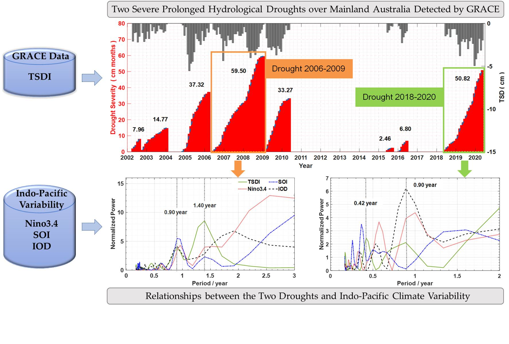
As shown in Figure 2, there are eight drought periods detected from the GRACE-based TSD time series over mainland Australia from April 2002 to May 2020, which have caused severe effects and got more attention at present [7,39]. The onset, termination and duration are summarized in Table 3 for the droughts over mainland Australia from April 2002 to May 2020. The first two most severe droughts that lasted for 32 months (from June 2006 to January 2009) and 24 months (from June 2018 to May 2020) are marked by the orange and green dotted line box in Figure 2, the correspondent drought severities are 59.50 and 50.82 (cm months) respectively. To facilitate the description, the two droughts are named Drought 2006–2009 and Drought 2018–2020 respectively.
3. Results
3.1. Drought Affected Area
The percentage of the drought-affected area relative to the total area over mainland Australia [66] is used to confirm whether the drought is continent-wide or regional. The percentages of the drought-affected area are presented in Figure 3. And the mean affected areas for Drought 2006–2009 and Drought 2018–2020 are 78% and 73% respectively. The affected area of Drought 2006–2009 ranged from 57% to 95% for all 32 months, while the affected area of Drought 2018–2020 ranged from 45% to 95%. Drought 2006–2009 and Drought 2018–2020 usually expanded to the maximum affected area in austral summer (from December to February). The affected area of Drought 2006–2009 reached its peak in December 2006 with a maximum of 95% and that of Drought 2018–2020 was in December 2019 with a maximum of 95%.
3.2. Drought Spatial Evolution
To show the spatial evolutions of Drought 2006–2009 and Drought 2018–2020, we calculate the mean TSDI every four months and showed them in Figure 4, where the red tone represents the drought condition caused by terrestrial water storage deficiency and the blue one represents the wet condition. The names and locations of six regions over mainland Australia are shown in the bottom-left of Figure 4. Drought 2006–2009 that lasted for 32 months is presented with eight upper sub-figures, and Drought 2018–2020 that lasted for 24 months is shown with six bottom sub-figures of Figure 4. From the eight upper sub-figures, we can observe that Drought 2006–2009 took its rise in southeastern Australia and gradually spread to the central part. Victoria and the Northern Territory suffered the most severe drought in terms of drought-affected areas and duration. In the six bottom sub-figures, Drought 2018–2020 originated in the southwest corner of the Northern Territory and northern New South Wales, and gradually expanded to Western Australia and the whole New South Wales respectively. The drought over Western Australia had been increasing until May 2020, but that of New South Wales disappeared in early 2020. The two hydrological droughts evolved and developed continually, yet the main affected areas of the two hydrological droughts were quite different.
3.3. Frequency of Different Drought Grades
The drought frequency is defined as the ratio of the months at a drought grade to the total months of the drought period. According to the drought grads in Table 2, only mild and moderate droughts are detected during Drought 2006–2009 and Drought 2018–2020 and the results are shown in Figure 5, where the frequency of mild drought is higher than that of moderate and also significantly different in the six regions. For Drought 2006–2009, the frequency of moderate droughts in Victoria was higher than in the other regions. Victoria and South Australia suffered drought all the months. Specifically, Victoria had 59% mild drought and 41% moderate drought while those of South Australia were 88% and 12% respectively. Since Drought 2006–2009 originated in the east and gradually developed to the center of mainland Australia, Western Australia had the least drought frequency. For Drought 2018–2020, Northern Territory was dominated by drought all the months, including 8% moderate drought and 92% mild drought and Victoria had the least drought frequency, while it had the highest drought frequency for Drought 2006–2009 (see the third pie in the upper of Figure 5).
3.4. Drought Severity
A drought with a short duration (less than three months) usually has a relatively small impact on water storage and agriculture, because the short-term deficit of water storage can be replenished by timely rainfall. However, continuous drought often leads to serious consequences, especially for agricultural production. The severity and duration of drought are comprehensively considered in the drought severity calculation and the drought severities for all six regions are shown in Table 4, with corresponding time and austral season (September to November for spring, December to February for summer, March to May for autumn, and June to August for winter).
The drought severities in North Territory are the highest among the 6 regions for both Drought 2006–2009 and Drought 2018–2020, with the severity of 44.26 and 52.19 (cm months) respectively. North Territory suffered the most serious drought. The drought severity in Victoria ranks the second for Drought 2006–2009, while that in South Australia is the lowest only with 10.78 (cm months). For Drought 2018–2020, the drought severity in Western Australia is the second high with 31.44 (cm months), while those in Queensland and Victoria are only about 11 (cm months). The highest drought severity usually generated in summer and winter for Drought 2006–2009, while for that of Drought 2018–2020 was in summer and autumn. Therefore, summer is normally the turning season with the most severe drought, and the hydrological conditions over mainland Australia usually change from drought to wet at the end of summer.
Temporal variability of drought severities in six regions is shown in Figure 6 for the two prolonged droughts. Same as that in Table 4, Northern Territory and Western Australia suffered severe drought while South Australia was affected the weakest. Besides, For Drought 2006–2009, Queensland had four drought periods, and other regions only had two or three periods. For Drought 2018–2020, all regions except for South Australia had two drought periods. Because drought severity is the cumulation of TSD during the drought period, longer drought duration and larger TSD will cause higher drought severity. For Drought 2018–2020, Northern Territory suffered the highest drought severity (52.19 cm months) because of very larger TSD, although the duration shorter than that in Western Australia. In other words, the hydrological drought severity in Northern Territory developed more violent than in West Australia.
3.5. Relationships between the Two Hydrological Droughts and Indo-Pacific Climate Variability
Temporal variability of Indo-Pacific climate indices with TSDI from April 2002 to May 2020 are shown in Figure 7 where the Drought 2006–2009 and Drought 2018–2020 are highlighted with orange and green backgrounds, respectively. From Figure 7 we can find that Nino3.4 and SOI during Drought 2006–2009 are more changeable and stronger than those during Drought 2018–2020. IOD is positive during almost all of the two droughts, consistent with that of Ummenhofer et al. [29] who found Australia usually experiences anomalous dry conditions during positive IOD events.
To quantify the influence of ENSO and IOD on Drought 2006–2009 and Drought 2018–2020 over mainland Australia, we first determine the lagging times between TSDI and the corresponding climate indices (Nino3.4, SOI and IOD) by maximizing the mean absolute value of correlation coefficients over mainland Australia. Then we fix the lagging times to compute the correlation coefficients over mainland Australia. Since the lagging times between TSDI and climate indices are not larger than seven months [26,28,64], we present the absolute correlation coefficients from zero to seven months in Figure 8 and summarize the determined lagging times in Table 5.
From Figure 8 we can observe that three correlation coefficients vary more obviously with different lagging times in the left figure than that in the right figure, which means that the lagging times determined for Drought 2006–2009 are probably better than that for Drought 2018–2020. Considering the differences of the three lagging times in Table 5 are only one month, the determined lagging times are reliable since TSDI is served from monthly GRACE data. Moreover, the correlation coefficients of Nino3.4 are larger than that of IOD in Figure 8a, which, however, is opposite in Figure 8b, hence Drought 2006–2009 is mainly driven by El Niño and Drought 2018–2020 is more impacted by IOD event. Comparing Drought 2018–2020 with Drought 2006–2009 we can see in Table 5 that the correlation coefficients of Nino3.4 reduce from 0.39 to 0.26, however those of IOD increase from 0.27 to 0.31. Therefore, over mainland Australia the impact of ENSO on the hydrological droughts may have decreased from 2002 to 2020, on the contrary, the impact of IOD has increased.
The correlation coefficients between TSDI and the indices for modes of Indo-Pacific climate variability (Nino3.4, SOI and IOD) over mainland Australia are shown in the upper and bottom of Figure 9 for Drought 2006–2009 and Drought 2018–2020, respectively. In Figure 9a, the correlations of Nino3.4 are very significant over western, northern and southeastern Australia for Drought 2006–2009, while those in Figure 9d only show in northwestern and southeastern Australia. Moreover, the patterns between Figure 9a,d are similar in the northwest and southeast areas. As for SOI, in Figure 9b strong negative correlations appear in Victoria, Northern Territory and northern Western Australia, strong positive correlations in southern Queensland and northern New South Wales, while in Figure 9e the correlation coefficients are more scattered with negative values in the northeast and positive in the other places. Furthermore, the patterns between Figure 9b,e are significantly different. In terms of IOD, similar correlations appear in the northwest and eastern edge in both Figure 9c,f, but opposite correlations in the southwest corner.
The mean absolute correlation coefficients between TSDI and three climate indices are shown in Figure 10 for the six regions (the orange represents Drought 2006–2009 and green is Drought 2018–2020). The correlation coefficient of SOI reaches 0.62 for Drought 2006–2009, significantly higher than that of Nino3.4 and IOD, hence SOI may play an important role for the drought in Victoria. Except for Victoria, the correlation coefficients of Nino3.4 for Drought 2006–2009 are larger than that for Drought 2018–2020 in all rest five regions. In addition, except for Northern Territory, the correlation coefficients of IOD for Drought 2018–2020 are larger than those for Drought 2006–2009 in all other five regions, which further confirm that the Drought 2006–2009 is mainly affected by El Niño and Drought 2018–2020 is more influenced by IOD.
4. Discussion
4.1. RMS of the Hydrological Drought Analysis
The RMS presented in Figure 11 is derived from the residuals of Equation (5) after removing the trends and seasonal terms, and the latitude weighted RMS values of the six regions are shown in Table 6. Since the residuals may still contain sub-seasonal and inter-annual signals, these RMS values may overestimate the actual uncertainties associated with the CSR mascon. As a whole, the RMS values over mainland Australia range from 0 to 3 cm. And they are relatively larger in northern mainland Australia and relatively smaller in the southwest. We can see from Figure 11 that the RMS near the equator is larger because the GRACE satellites are polar-orbiting and the spatial sampling in the equator is relatively sparse [67,68]. Besides, it may also because the larger inter-annual variation of terrestrial water storage in the Northern Territory makes its RMS larger. For the region scale, the RMS in the Northern Territory is 2.11 cm, and those of other regions are less than 1.5 cm, which is consistent with the present accuracy of the GRACE data (cm level).
4.2. Comparison of Drought 2006–2009 and Drought 2018–2020
First, we compared the results of the linkage between the two droughts and the Indo-Pacific climate variability with the previous study. The two hydrological droughts in northern and eastern mainland Australia are influenced by ENSO since significant correlations are between TSDI and both of Nino3.4 and SOI over the two droughts (see Figure 9), consistent with Risbey et al. [33] who found ENSO is related to rainfall over much of the continent at different times, particularly in the north and east [33]. Moreover, Forootan et al. [69] found a strong presence of ENSO-induced TWS derived from GRACE data over Australia is increasing from 1990 to 2010 (Drought 2006–2009 in this work) and IOD-induced TWS is increasing from 2004 to 2014. We find that the hydrological drought in the southwestern corner of mainland Australia is primarily influenced by Pacific climate variability during Drought 2006–2009, but with the stronger impact of IOD for Drought 2018–2020. The large precipitation variations associated with ENSO and IOD were found over the northern and northeast coast during 2002–2011 [26], but we found that the TSDI in the northeast coast has little linkage with ENSO and IOD. One reason to accounts for this is that TSDI is also influenced by evapotranspiration and runoff, which may lead to the differences between precipitation and hydrological drought derived from GRACE-based TWS [70]. Besides, the study periods here are determined based on the drought severity over mainland Australia and they are different from that of [26], which may also lead to the difference.
Furthermore, we analyzed the spatial pattern of the correlation characteristic and tried to give the prediction of the impact of ENSO and IOD on both of the two droughts, northern and eastern mainland Australia were impacted by El Niño and IOD, indicating the relatively stable impacts of them. So, we can carefully deduce that the hydrological drought in northern and eastern mainland Australia may still be related to the changes of El Niño and IOD variability in the future. The role of Southern Oscillation is diverse, for Drought 2006–2009, the correlation coefficients of TSDI and SOI in western and central parts of Australia are negative and that in the northeastern part are positive. However, for Drought 2018–2020, the pattern is opposite, indicating the more complex and diverse driving mechanism of Southern Oscillation. And these conclusions are consistent with the findings that ocean-based ENSO indices (e.g., Nino3.4) are more skillful as predictors of Australian rainfall than the SOI at a longer lead time [71]. And the correlation coefficients between TSDI and both of Nino3.4 and IOD in western, northern and central parts of mainland Australia are negative, and those of the other places are positive, this phenomenon was also shown in [26,33]. It should be noted that isolating the physical mechanisms through which a specific global climate index might influence the hydrological droughts is beyond the scope of the present study. Instead, the study focused on isolating the possible influence of global climate indices and teleconnections on TSDI over mainland Australia based on the correlation analysis for the two hydrological droughts.
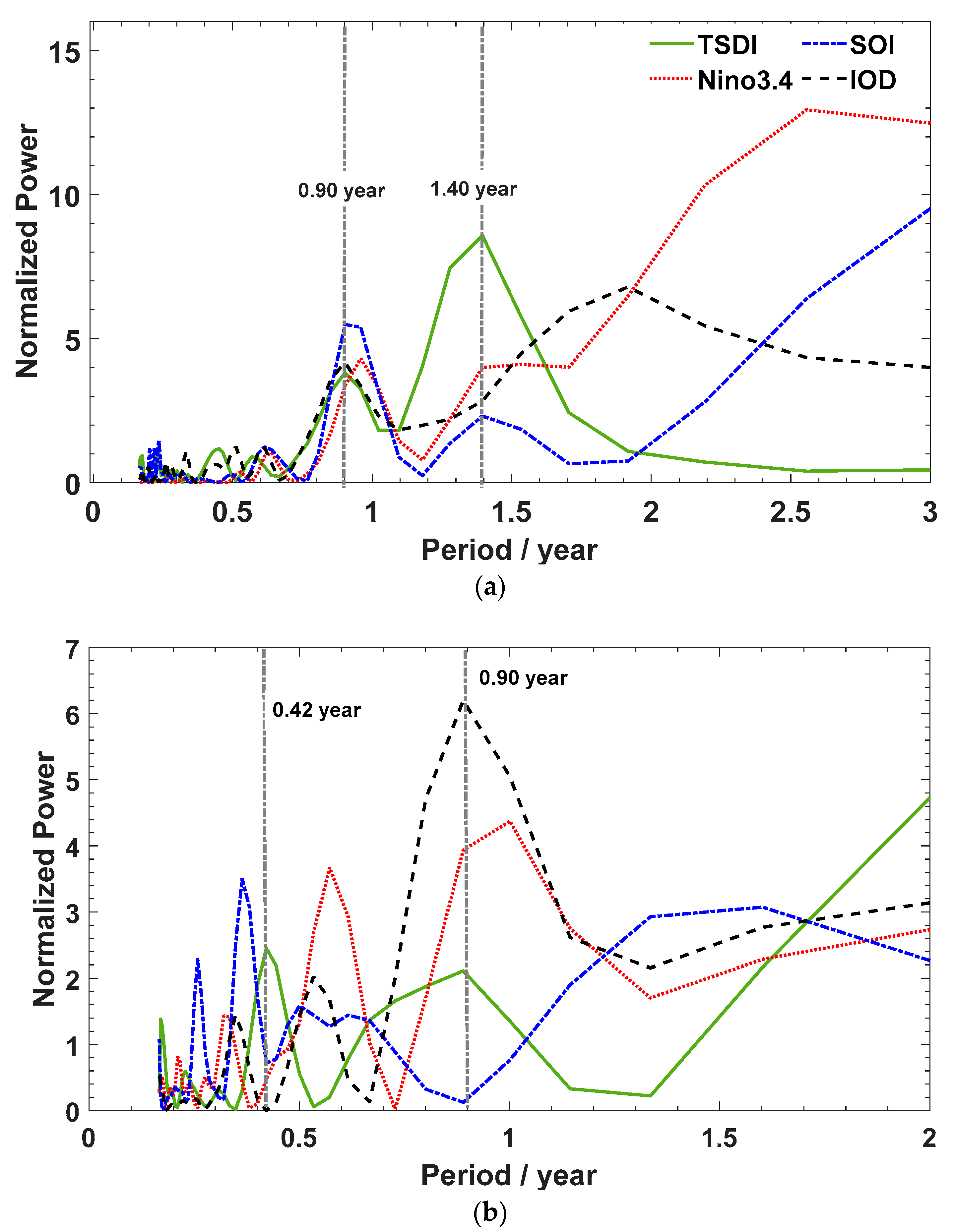
To explore the non-linear relationships between the two hydrological droughts and Indo-Pacific climate variability, we further use the Fourier analysis to analyze the four indices (TSDI, Nino3.4, SOI and IOD) over the periods of the two hydrological droughts. The corresponding power spectra are shown in Figure 12. For Drought 2006–2009, the power spectrum of TSDI matches well with that of Indo-Pacific climate variability at the period about 0.90 years and also matches that of SOI at the period about 1.40 years, which shows that Drought 2006–2009 was driven by Indo-Pacific climate variability to some extent. However, for Drought 2018–2020, the power spectrum of TSDI matches with that of Nino3.4 and IOD well at the period about 0.90 years but approximately matches with that of SOI at the period about 0.42 years, confirming a slight difference of driving mechanism between Drought 2006–2009 and Drought 2018–2020.
5. Conclusions
Focusing on two severe and prolonged droughts over mainland Australia, this paper analyzed the hydrological droughts from the perspective of the affected area, spatial evolution, frequency, severity as well as the relationship between hydrological droughts and Indo-Pacific climate indices.
The percentages of affected areas of total mainland Australia for Drought 2006–2009 range from 57% to 95%, while those of Drought 2018–2020 were from 45% to 95%. As for the spatial evolutions of the two droughts, Drought 2006–2009 took its rise in southeastern mainland Australia and gradually spread to the interior. Drought 2018–2020 originated in the southwest corner of the Northern Territory and northern New South Wales, and gradually expanded to Western Australia and New South Wales respectively. For Drought 2006–2009, Victoria and South Australia suffered drought for all 32 months. The mild and moderate droughts in Victoria were 59% and 41%, while those in South Australia were 88% and 12% respectively. Yet Western Australia had the least number of drought months among the six regions. For Drought 2018–2020, Northern Territory was dry all the months, including 8% moderate and 92% mild drought respectively. The drought severities of North Territory during Drought 2006–2009 and 2018–2020 were both the highest than the other regions, with the severities of 44.26 and 52.19 (cm months) respectively. For Drought 2006–2009, the drought severity of Victoria ranked the second, while that of South Australia was the lowest. For Drought 2018–2020, the drought severity of Western Australia was the second high, while those of Queensland and Victoria were both the lowest. Considering the drought season, we found that summer is usually the turning season with the most severe droughts, and the hydrological conditions over mainland Australia usually change from drought to wet at the end of summer. The correlation patterns of El Niño are similar in the northwest and southeast areas for the two droughts, while that of SOI are significantly different. For IOD, correlation patterns are similar in the northwest and eastern edge, but with opposite correlations in the southwest corner. The impacts of Pacific climate variability on the hydrological droughts have decreased from Drought2006–2009 to Drought 2018–2020, on the contrary, the impact of Indo climate variability has increased. The results of Fourier analysis show that the two hydrological droughts are all related to Indo-Pacific climate variability, while the driving mechanism of Drought 2018–2020 is slightly different from that of Drought 2018–2020 to some extent.
Author Contributions
Y.S. proposed the key idea, supervised the research, and revised the paper; W.W. carried out the data analysis and wrote the paper; F.W. and W.L. revised the manuscript. All authors have read and agreed to the published version of the manuscript.
Funding
This research is funded by the National Natural Science Foundation of China (41974002) and the National Key R&D Program of China (2017YFA0603103).
Acknowledgments
The authors thank GRACE data processing center CSR for providing the GRACE data. We also acknowledge the careful and constructive reviews of Academic Editor: Christian Massari and Magaly Koch, Assistant Editor Crystal Kuang, and five anonymous reviewers, who have helped improve the manuscript.
Conflicts of Interest
The authors declare no conflict of interest.
References
- Rashid, M.M.; Simon Beecham, S. Characterization of meteorological droughts across South Australia. Meteorol. Appl. 2019, 26, 556–568. [Google Scholar] [CrossRef] [Green Version]
- Alkaisi, M.M.; Elmore, R.W.; Guzman, J.G.; Hanna, H.M.; Hart, C.E.; Helmers, M.J.; Hodgson, E.W.; Lenssen, A.W.; Mallarino, A.P.; Robertson, A.E.; et al. Drought impact on crop production and the soil environment: 2012 experiences from lowa. Soil Water Conserv. 2013, 68, 19A–24A. [Google Scholar] [CrossRef] [Green Version]
- Frank, A.; Armenski, T.; Gocic, M.; Popov, S.; Popovic, L.; Trajkovic, S. Influence of mathematical and physical background of drought indices on their complementarity and drought recognition ability. Atmos. Res. 2017, 194, 268–280. [Google Scholar] [CrossRef]
- Mo, K.C. Drought onset and recovery over the United States. J. Geophys. Res. Atmos. 2011, 116, 1–14. [Google Scholar] [CrossRef]
- Vu, M.T.; Vo, N.D.; Gourbesville, P.; Raghavan, S.V.; Liang, S.-Y. Hydro-meteorological drought assessment under climate change impact over the Vu Gia-Thu Bon river basin, Vietnam. Hydrol. Sci. J. 2017, 62, 1654–1668. [Google Scholar] [CrossRef]
- Spinoni, J.; Barbosaa, P.; Jagera, A.D.; McCormicka, N.; Naumanna, G.; Vogta, J.V.; Magnib, D.; Masanteb, D.; Mazzeschic, M. A new global database of meteorological drought events from 1951 to 2016. J. Hydrol. Reg. Stud. 2019, 22, 100593. [Google Scholar] [CrossRef]
- Leblanc, M.; Tweed, S.; Dijk, A.V.; Timbal, B. A review of historic and future hydrological changes in the Murray-Darling Basin. Glob. Planet. Chang. 2012, 80–81, 226–246. [Google Scholar] [CrossRef]
- Van Dijk, A.I.J.M.; Beck, H.E.; Crosbie, R.S.; de Jeu, R.A.M.; Liu, Y.Y.; Podger, G.M.; Timbal, B.; Viney, N.R. The Millennium Drought in southeast Australia (2001–2009): Natural and human causes and implications for water resources, ecosystems, economy, and society. Water Resour. Res. 2013, 49, 1040–1057. [Google Scholar] [CrossRef]
- Kauwe, M.G.D.; Medlyn, B.E.; Ukkola, A.M.; Mu, M.; Sabot, M.E.B.; Pitman, A.J. Identifying areas at risk of drought-induced tree mortality across South-Eastern Australia. Glob. Chang. Biol. 2020, 26, 5716–5733. [Google Scholar] [CrossRef]
- Creutzfeldt, B.; Ferré, T.; Troch, P.; Merz, B.; Wziontek, H.; Güntner, A. Total water storage dynamics in response to climate variability and extremes: Inference from long-term terrestrial gravity measurement. J. Geophys. Res. Atmos. 2012, 117, D08112. [Google Scholar] [CrossRef] [Green Version]
- Thomas, A.C.; Reager, J.T.; Famiglietti, J.S.; Rodell, M. A GRACE-based water storage deficit approach for hydrological drought characterization. Geophys. Res. Lett. 2014, 41, 1537–1545. [Google Scholar] [CrossRef] [Green Version]
- Wahr, J.; Swenson, S.; Zlotnicki, V.; Velicogna, I. Time-Variable gravity from GRACE: First Results. Geophys. Res. Lett. 2004, 31, L11501. [Google Scholar] [CrossRef] [Green Version]
- Chen, J.L.; Wilson, C.R.; Tapley, B.D.; Scanlon, B.; Güntner, A. Long-term groundwater storage change in Victoria, Australia from satellite gravity and in situ observations. Glob. Planet. Chang. 2016, 139, 56–65. [Google Scholar] [CrossRef] [Green Version]
- Wang, S.S. Freezing temperature controls winter water discharge for cold region watershed. Water Resour. Res. 2019, 55, 479–493. [Google Scholar] [CrossRef] [Green Version]
- Doumbia, C.; Castellazzi, P.; Rousseau, A.N.; Amaya, M. High Resolution Mapping of Ice Mass Loss in the Gulf of Alaska From Constrained Forward Modeling of GRACE Data. Front. Earth Sci. 2020, 7, 360. [Google Scholar] [CrossRef]
- Zhang, L.S.; Zhu, X.F.; Pan, Y.Z.; Zhang, J.S. Assessing Terrestrial Water Storage and Flood Potential Using GRACE Data in the Yangtze River Basin, China. Remote Sens. 2017, 9, 1011. [Google Scholar]
- Cao, Y.P.; Nan, Z.T.; Cheng, G.D. GRACE Gravity Satellite Observations of Terrestrial Water Storage Changes for Drought Characterization in the Aid Land of Northwestern China. Remote Sens. 2015, 7, 1021–1047. [Google Scholar] [CrossRef] [Green Version]
- Sun, Z.L.; Zhu, X.F.; Pan, Y.Z.; Zhang, J.S.; Liu, X.F. Drought evaluation using the GRACE terrestrial water storage deficit over the Yangtze River Basin, China. Sci. Total Environ. 2018, 634, 727–738. [Google Scholar] [CrossRef]
- Liu, X.F.; Feng, X.M.; Ciais, P.; Fu, B.J.; Hu, B.Y.; Sun, Z.L. GRACE satellite-based drought index indicating increased impact of drought over major basins in China during 2002–2007. Agric. For. Meteorol. 2020, 291, 108057. [Google Scholar] [CrossRef]
- Sinha, D.; Syed, T.H.; Famiglietti, J.S.; Reager, J.T.; Thomas, R.C. Characterizing drought in India using GRACE observations of terrestrial water storage deficit. J. Hydrometeorol. 2017, 18, 381–396. [Google Scholar] [CrossRef]
- Sinha, D.; Syed, T.H.; Reager, J.T. Utilizing combined deviations of precipitation and GRACE-based terrestrial water storage as a metric for drought characterization: A case study over major Indian river basins. J. Hydrol. 2019, 572, 294–307. [Google Scholar] [CrossRef]
- Yu, W.J.; Li, Y.Z.; Cao, Y.P.; Schillerberg, T. Drought Assessment using GRACE Terrestrial Water Storage Deficit in Mongolia from 2002 to 2017. Water 2019, 11, 1301. [Google Scholar] [CrossRef] [Green Version]
- Jing, W.L.; Zhao, X.D.; Yao, L.; Jiang, H.; Xu, J.H.; Yang, J.; Li, Y. Variations in terrestrial water storage in the Lancang-Mekong river basin from GRACE solutions and land surface model. J. Hydrol. 2020, 580, 124258. [Google Scholar] [CrossRef]
- Chaudhari, S.; Pokhrel, Y.; Moran, E.; Miguez-Macho, G. Multi-decadal hydrologic change and variability in the Amazon River basin: Understanding terrestrial water storage variations and drought characteristics. Hydrol. Earth Syst. Sci. 2019, 23, 2841–2862. [Google Scholar] [CrossRef] [Green Version]
- Hosseini-Moghari, S.-M.; Araghinejad, S.; Ebrahimi, K.; Tourian, M.J. Introducing modified total storage deficit index (MTSDI) for drought monitoring using GRACE observations. Ecol. Indic. 2019, 101, 465–475. [Google Scholar] [CrossRef]
- Forootan, E.; Khandu Awange, J.L.; Schumacher, M.; Anyah, R.; van Dijk, A.I.J.M.; Kusche, J. Quantifying the impacts of ENSO and IOD on rain gauge and remotely sensed precipitation products over Australia. Remote Sens. Environ. 2016, 172, 50–66. [Google Scholar] [CrossRef] [Green Version]
- Forootan, E.; Khaki, M.; Schumacher, M.; Wulfmeyer, V.; Mehrnegar, N.; van Dijk, A.I.J.M.; Brocca, L.; Farzaneh, S.; Akinluyi, F.; Ramillien, G.; et al. Understanding the global hydrological droughts of 2003–2016 and their relationships with teleconnections. Sci. Total Environ. 2019, 650, 2587–2604. [Google Scholar] [CrossRef] [Green Version]
- Allen, K.J.; Freund, M.B.; Palmer, J.G.; Williams, L.; Brookhouse, M.; Cook, R.E.; Stewart, S.; Backer, P.J. Hydroclimate extremes in a north Australian drought reconstruction asymmetrically linked with Central Pacific Sea surface temperatures. Glob. Planet. Change 2020, 195, 103329. [Google Scholar] [CrossRef]
- Ummenhofer, C.C.; England, M.H.; McIntosh, M.C.; Meyers, G.A.; Pook, M.J.; Risbey, J.S.; Gupta, A.S.; Taschetto, A.S. What causes southeast Australia’s worst droughts? Geophys. Res. Lett. 2009, 36, L04706. [Google Scholar] [CrossRef] [Green Version]
- Cai, W.J.; Cowan, T. Dynamics of late autumn rainfall reduction over southeastern Australia. Geophys. Res. Lett. 2008, 35, L09708. [Google Scholar] [CrossRef]
- Cai, W.J.; Cowan, T.; Raupach, M. Positive Indian Ocean Dipole events precondition southeast Australia bushfires. Geophys. Res. Lett. 2009, 36, L19710. [Google Scholar] [CrossRef]
- Saji, N.H.; Goswami, B.N.; Vinayachandran, P.N.; Yamagata, T. A dipole mode in the tropical Indian Ocean. Nature 1999, 401, 360–363. [Google Scholar] [CrossRef] [PubMed]
- Risbey, J.S.; Pook, M.J.; Mcintosh, P.C. On the Remote Drivers of Rainfall Variability in Australia. Bull. Am. Meteorol. Soc. 2009, 137, 3233–3253. [Google Scholar] [CrossRef]
- Hu, T.; van Dijk, A.I.J.M.; Renzullo, L.J.; Xu, Z.H.; He, J.; Tian, S.; Zhou, J.; Li, H. On agricultural drought monitoring in Australia using Himawari-8 geostationary thermal infrared observations. Int. J. Appl. Earth Obs. 2020, 91, 102153. [Google Scholar] [CrossRef]
- Yang, Y.; Long, D.; Guan, H.; Scanlon, B.R.; Simmons, C.T.; Jiang, L.; Xu, X. GRACE satellite observed hydrological controls on interannual and seasonal variability in surface greenness over mainland Australia. J. Geophys. Res. Biogeosci. 2014, 119, 2245–2260. [Google Scholar] [CrossRef]
- Chen, T.; de Jeu, R.A.M.; Liu, Y.Y.; van der Werf, G.R.; Dolman, A.J. Using satellite based soil moisture to quantify the water driven variability in NDVI: A case study over mainland Australia. Remote Sens. Environ. 2014, 140, 330–338. [Google Scholar] [CrossRef]
- Leblanc, M.J.; Tregoning, P.; Ramillien, G.; Tweed, S.O.; Fakes, A. Basin-scale, integrated observations of the early 21st century multiyear drought in southeast Australia. Water Resour. Res. 2009, 45, W04408. [Google Scholar] [CrossRef]
- Köppen, W. Die Wärmezonen der Erde, nach der Dauer der Heissen, Gemässigten, und Kalten Zeit, und nach der Wirkung der Wärme auf die Organisch Welt betrachtet. Meteorol. Z. 1884, 1, 215–226. Available online: http://www.metvis.com.au/acc/index.html (accessed on 22 February 2021).
- Feng, T.; Wu, J.J.; Liu, L.Z.; Leng, S.; Yang, J.H.; Zhao, W.H.; Shen, Q. Exceptional Drought across Southeastern Australia Caused by Extreme Lack of Precipitation and Its Impacts on NDVI and SIF in 2018. Remote Sens. 2020, 12, 54. [Google Scholar]
- Mohamad, N.; Md Din, A.H. Monitoring Groundwater Depletion Due to Drought using Satellite Gravimetry: A Review. IOP Conf. Ser. Earth Environ. Sci. 2020, 540, 012054. [Google Scholar] [CrossRef]
- Tapley, B.D.; Bettadpur, S.; Ries, J.C.; Thompson, P.F.; Watkins, M.M. GRACE Measurements of Mass Variability in the Earth System. Science 2004, 305, 503–505. [Google Scholar] [CrossRef] [Green Version]
- Verdon-Kidd, D.C.; Kiem, A.S. Nature and causes of protracted droughts in southeast Australia: Comparison between the Federation, WWII, and Big Dry droughts. Geophys. Res. Lett. 2009, 36, L22707. [Google Scholar] [CrossRef]
- Dikshit, A.; Pradhan, B.; M. Alamr, A. Short-Term Spatio-Temporal Drought Forecasting Using Random Forests Model at New South Wales, Australia. Appl. Sci. 2020, 10, 4254. [Google Scholar] [CrossRef]
- Shi, L.J.; Feng, P.Y.; Wang, B.; Liu, D.L.; Yu, Q. Quantifying future drought change and associated uncertainty in southeastern Australia with multiple potential evapotranspiration models. J. Hydrol. 2020, 590, 125394. [Google Scholar] [CrossRef]
- Rahmat, S.N.; Jayasuriya, N.; Bhuiyan, M. Assessing droughts using meteorological drought indices in Victoria, Australia. Hydrol. Res. 2015, 46, 463–476. [Google Scholar] [CrossRef]
- Zhao, M.; Geruo, A.; Velicogna, I.; Kimball, J.S. A Global Gridded Dataset of GRACE Drought Severity Index for 2002–14: Comparison with PDSI and SPEI and a Case Study of the Australia Millennium Drought. J. Hydrometeorol. 2017, 18, 2117–2129. [Google Scholar] [CrossRef] [Green Version]
- Save, H.; Bettadpur, S.; Tapley, B.D. High-resolution CSR GRACE RL05 mascons. J. Geophys. Res. Solid Earth 2016, 121, 7547–7569. [Google Scholar] [CrossRef]
- Save, H. CSR GRACE and GRACE-FO RL06 Mascon Solutions v02. 2020. Available online: http://www2.csr.utexas.edu/grace/RL06_mascons.html (accessed on 22 February 2021). [CrossRef]
- Rangelova, E.; van der Wal, W.; Sideris, M.G.; Wu, P.B. Gravity, Geoid and Earth Observation; International Association of Geodesy Symposia; Springer: Berlin/Heidelberg, Germany, 2010; pp. 539–546. [Google Scholar]
- Watkins, M.M.; Wiese, D.N.; Yuan, D.-N.; Boening, C.; Landerer, F.W. Improved methods for observing Earth’s time variable mass distribution with GRACE using spherical cap mascons. J. Geophys. Res. Solid Earth 2015, 120, 2648–2671. [Google Scholar] [CrossRef]
- Solander, K.C.; Reager, J.T.; Wada, Y.; Famiglietti, J.S.; Middleton, R.S. GRACE satellite observations reveal the severity of recent water overconsumption in the United States. Sci. Rep. 2017, 7, 8723. [Google Scholar] [CrossRef] [PubMed] [Green Version]
- Cai, W.J.; van Rensch, P.; Cowan, T.; Hendon, H.H. An asymmetry in the IOD and ENSO teleconnection pathway and its impact on Australian climate. J. Clim. 2012, 25, 6318–6329. [Google Scholar] [CrossRef]
- Trenberth, K.E. Recent observed interdecadal climate changes in the Northern Hemisphere. Bull. Am. Meteorol. Soc. 1990, 71, 988–993. [Google Scholar] [CrossRef] [Green Version]
- Kim, T.W.; Valdes, J.B.; Nijssen, B.; Roncayolo, D. Quantification of linkages between large-scale climatic patterns and precipitation in the Colorado River Basin. J. Hydrol. 2006, 321, 173–186. [Google Scholar] [CrossRef]
- Saji, N.H.; Yamagata, T. Possible impacts of Indian Ocean dipole mode events on global climate. Clim. Res. 2003, 25, 151–169. [Google Scholar] [CrossRef]
- Rayner, N.A.; Parker, D.E.; Horton, E.B.; Folland, C.K.; Alexander, L.V.; Rowell, D.P.; Kent, E.C.; Kaplan, A. Global analyses of sea surface temperature, sea ice, and night marine air temperature since the late nineteenth century. J. Geophys. Res. 2003, 108, 4407. [Google Scholar] [CrossRef]
- Allan, R.J.; Nicholls, N.; Jones, P.D.; Butterworth, I.J. A further extension of the Tahiti-Darwin SOI, early SOI results and Darwin pressure. J. Clim. 1991, 4, 743–749. [Google Scholar] [CrossRef]
- Können, G.P.; Jones, P.D.; Kaltofen, M.H.; Allan, R.J. Pre-1866 extensions of the Southern Oscillation Index using early Indonesian and Tahitian meteorological readings. J. Clim. 1998, 11, 2325–2339. [Google Scholar] [CrossRef]
- Ropelewski, C.F.; Jones, P.D. An extension of the Tahiti-Darwin Southern Oscillation Index. Mon. Weather Rev. 1987, 115, 2161–2165. [Google Scholar] [CrossRef] [Green Version]
- Herring, S.C.; Christidis, N.; Hoell, A.; Kossin, J.P.; Schreck III, C.J.; Stott, P.A. Explaining extreme events of 2016 from a climate perspective. Bull.Am. Meteorol. Soc. 2018, 99, S1–S157. [Google Scholar] [CrossRef] [Green Version]
- Wanders, N.; Van Lanen, H.A.J.; van Loon, A.F. Indicators for Drought Characterization on Global Scale; Technical Report No. 24. 2010. Available online: https://library.wur.nl/WebQuery/wurpubs/fulltext/160049 (accessed on 22 February 2021).
- Nicholls, N. Sea surface temperature and Australian winter rainfall. J. Clim. 1989, 2, 965–973. [Google Scholar] [CrossRef] [Green Version]
- Knapp, C.H.; Carter, G.C.E.F. The Generalized Correlation Method for Estimation of Time Delay. IEEE Trans. Acoust. Speech Signal Process. 1976, 24, 320–327. [Google Scholar] [CrossRef] [Green Version]
- Rieser, D.; Kuhn, M.; Pail, R.; Anjasmara, I.M.; Awange, J. Relation between GRACE-derived surface mass variations and precipitation over Australia. Aust. J. Earth Sci. 2010, 57, 887–900. [Google Scholar] [CrossRef]
- Cleveland, R.B.; Cleveland, W.S.; Terpenning, I. STL: A seasonal-trend decomposition procedure based on loess. J. Off. Stat. 1990, 6, 3–73. [Google Scholar]
- Mishra, A.K.; Singh, V.P. A Review of drought concepts. J. Hydrol. 2010, 391, 202–216. [Google Scholar] [CrossRef]
- Schmidt, R.; Flechtner, F.; Meyer, F.; Neumayer, K.-H.; Dahle, C.H.; König, R.; Kusche, J. Hydrological Signals Observed by the GRACE Satellites. Surv. Geophys. 2008, 29, 319–334. [Google Scholar] [CrossRef]
- Wahr, J.; Swenson, S.; Velicogna, I. Accuracy of GRACE mass estimates. Geophys. Res. Lett. 2006, 33, L06401. [Google Scholar] [CrossRef] [Green Version]
- Forootan, E.; Kusche, J.; van Dijk, A.; Awange, J.L.; Schumacher, M.; Longuevergne, L. Non-stationary relationships between decadal water storage changes over Australia and climate variability of the El Niño Southern Oscillation and Indian Ocean Dipole. In Proceedings of the EGU General Assembly 2014, Vienna, Austria, 27 April–2 May 2014; Volume 16. EGU2014-4290. Available online: https://meetingorganizer.copernicus.org/EGU2014/EGU2014-4290.pdf (accessed on 22 February 2021).
- Anyah, R.O.; Forootan, E.; Awange, J.L.; Khaki, M. Understanding linkages between global climate indices and terrestrial water storage changes over Africa using GRACE products. Sci. Total Environ. 2018, 635, 1405–1416. [Google Scholar] [CrossRef] [PubMed] [Green Version]
- Lo, F.; Wheeler, M.; Meinke, H.; Donald, A. Probabilistic forecasts of the onset of the north Australian wet season. Mon. Wea. Rev. 2007, 135, 3506–3520. [Google Scholar] [CrossRef] [Green Version]
Figure 1.
The Köppen climate classification for Australia.

Figure 2.
Durations and severities of drought periods over mainland Australia from April 2002 to May 2020 (The red bar: drought severity; the gray bar: total water storage deficit).
Figure 2.
Durations and severities of drought periods over mainland Australia from April 2002 to May 2020 (The red bar: drought severity; the gray bar: total water storage deficit).
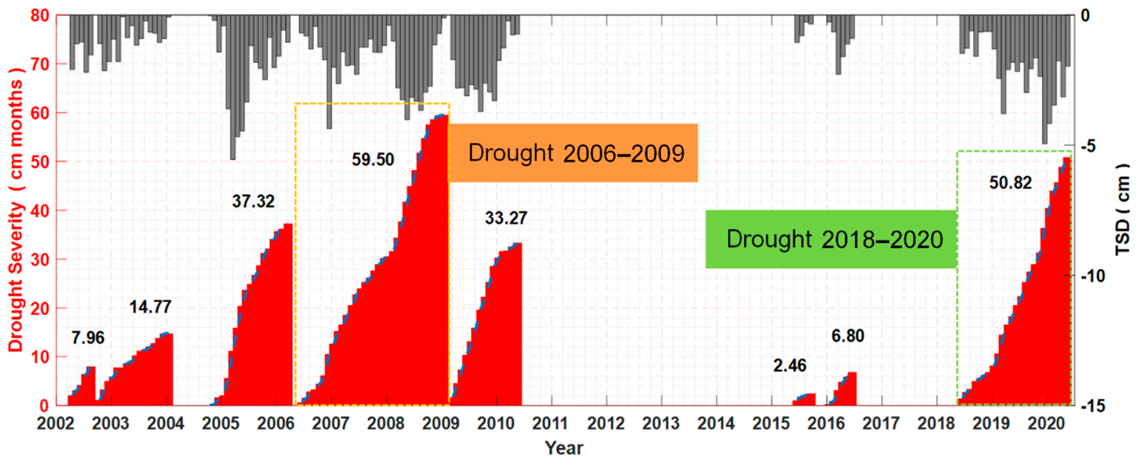
Figure 3.
Percentages of drought-affected area for Drought 2006–2009 (Left—Orange) and Drought 2018–2020 (Right—Green).
Figure 3.
Percentages of drought-affected area for Drought 2006–2009 (Left—Orange) and Drought 2018–2020 (Right—Green).
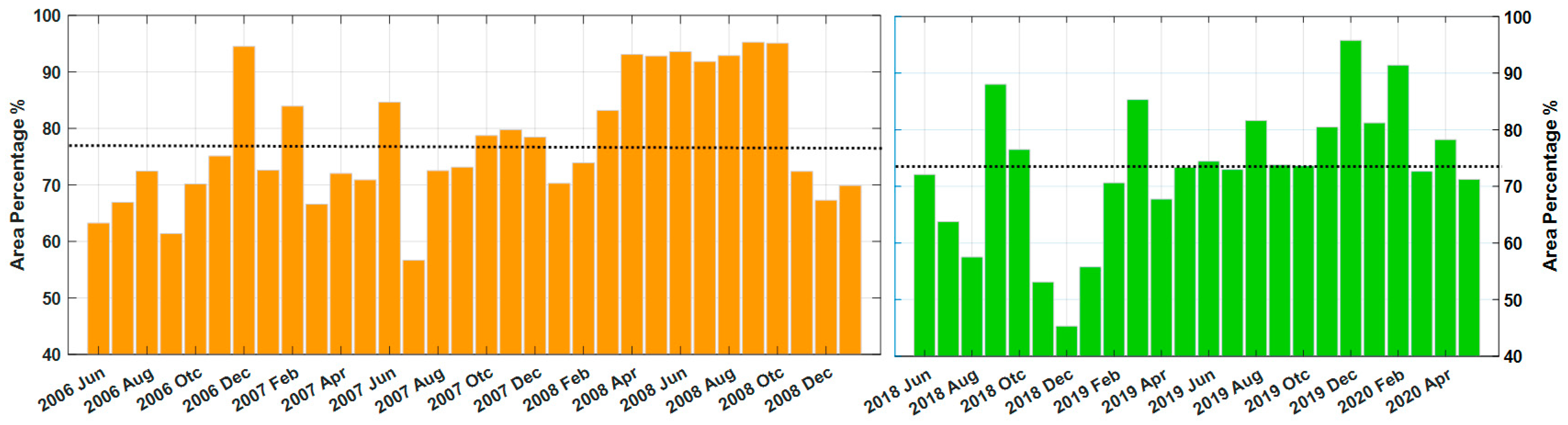
Figure 4.
Spatial distributions of the evolution for droughts reflected by TSDI during Drought 2006–2009 and Drought 2018–2020. (The sub-figures of mean TSDI are calculated every four months, the red tone represents drought, and the blue tone represents wet condition).
Figure 4.
Spatial distributions of the evolution for droughts reflected by TSDI during Drought 2006–2009 and Drought 2018–2020. (The sub-figures of mean TSDI are calculated every four months, the red tone represents drought, and the blue tone represents wet condition).
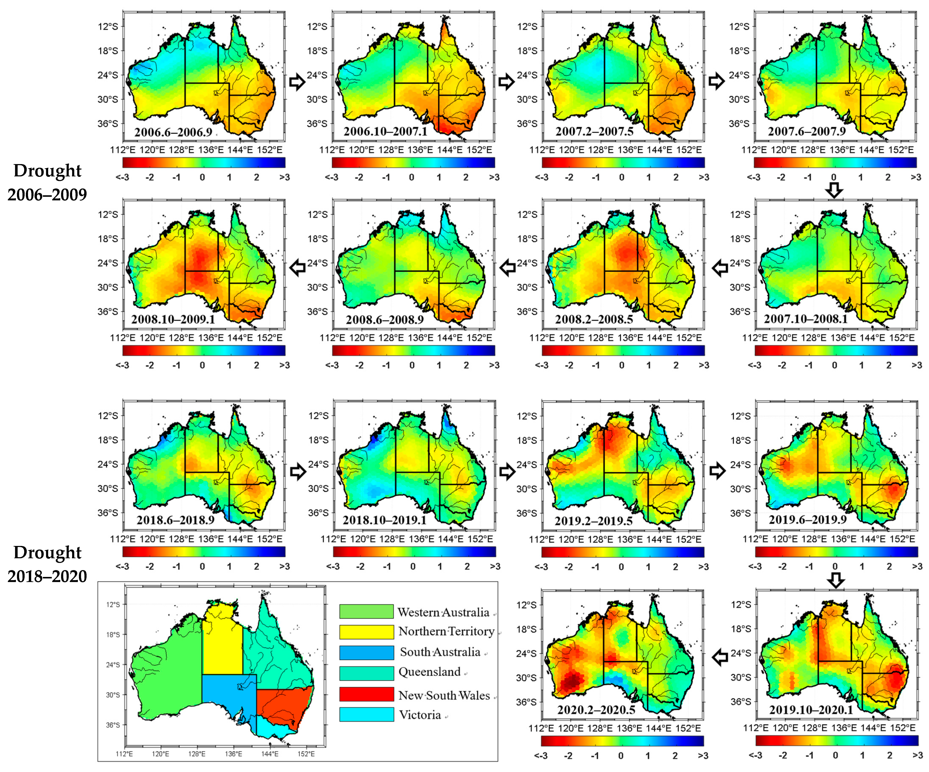
Figure 5.
Drought frequency among the six regions during Drought 2006–2009 and 2018–2020 (Note: the yellow part represents mild droughts and the orange part represents moderate droughts).
Figure 5.
Drought frequency among the six regions during Drought 2006–2009 and 2018–2020 (Note: the yellow part represents mild droughts and the orange part represents moderate droughts).
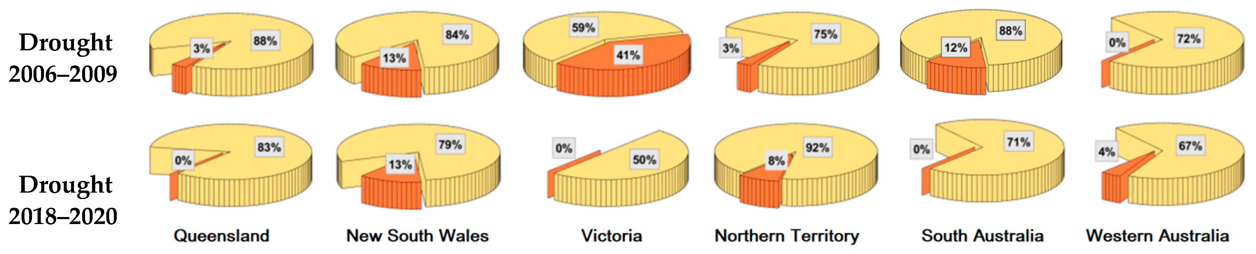
Figure 6.
Drought severities among 6 regions during Drought 2006–2009 and Drought 2018–2020.
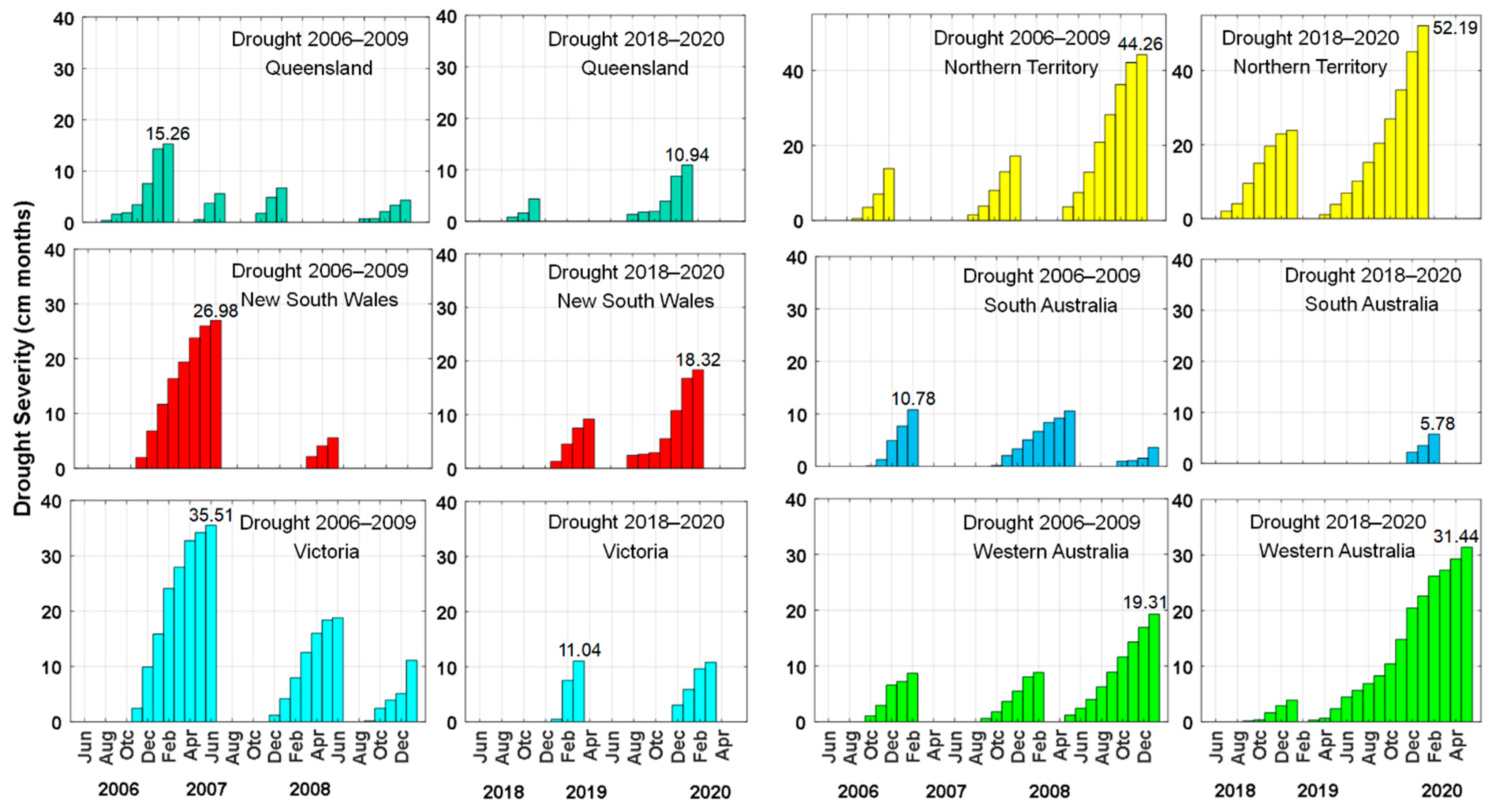
Figure 7.
Temporal variability of Indo-Pacific climate indices (a) Nino3.4 (b) SOI and (c) IOD with TSDI from April 2002 to May 2020 (The orange background represents Drought 2006–2009 and the green background represents Drought 2018–2020).
Figure 7.
Temporal variability of Indo-Pacific climate indices (a) Nino3.4 (b) SOI and (c) IOD with TSDI from April 2002 to May 2020 (The orange background represents Drought 2006–2009 and the green background represents Drought 2018–2020).

Figure 8.
The mean amount of correlation coefficients between TSDI and drought driving factors over mainland Australia during (a) Drought 2006–2009; (b) Drought 2018–2020.
Figure 8.
The mean amount of correlation coefficients between TSDI and drought driving factors over mainland Australia during (a) Drought 2006–2009; (b) Drought 2018–2020.

Figure 9.
The correlation coefficients between TSDI and drought driving factors. Upper: Drought 2006–2009; bottom: Drought 2018–2020. (a,d) represent for Nino3.4; (b,e) SOI; (c,f) for IOD.
Figure 9.
The correlation coefficients between TSDI and drought driving factors. Upper: Drought 2006–2009; bottom: Drought 2018–2020. (a,d) represent for Nino3.4; (b,e) SOI; (c,f) for IOD.
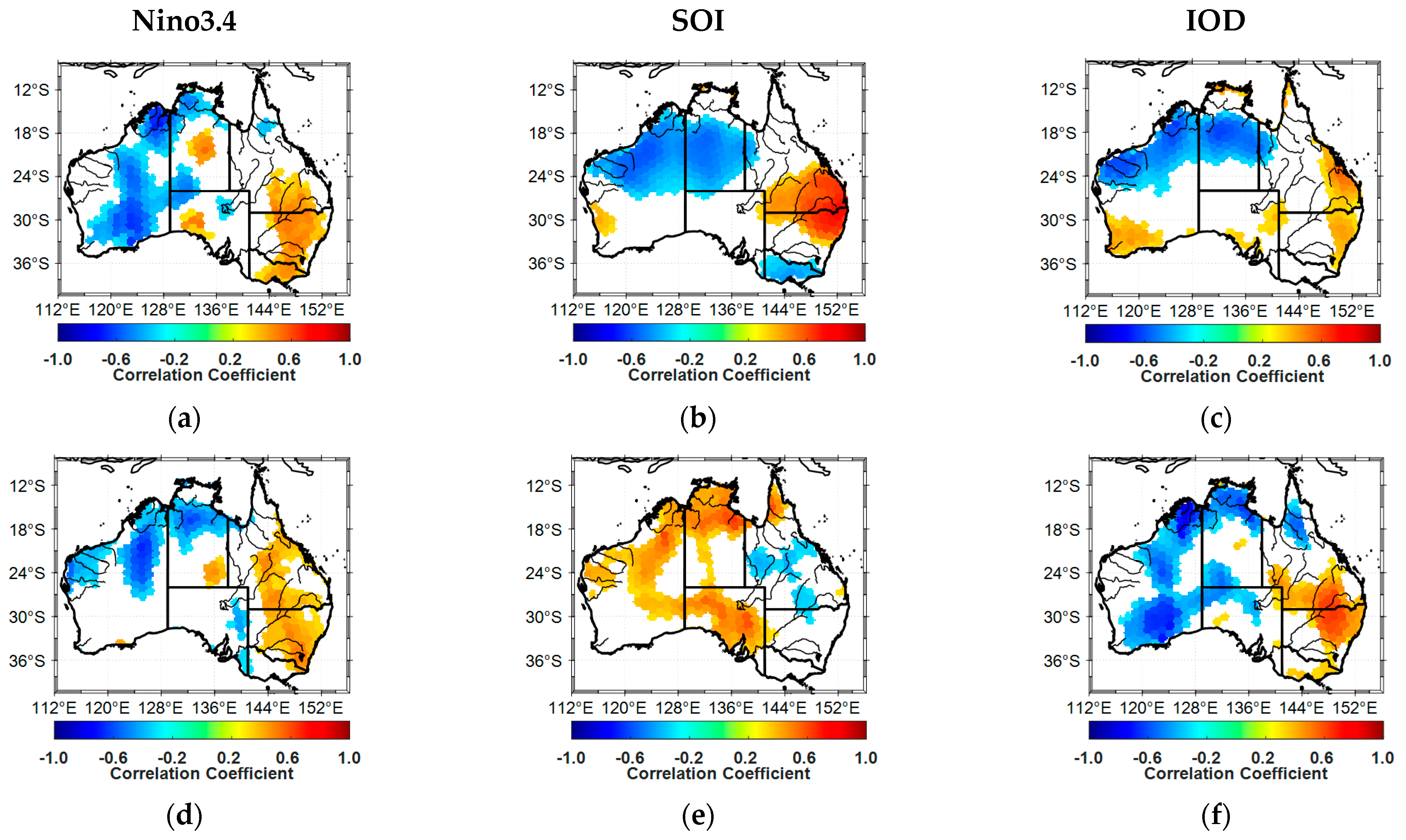
Figure 10.
The influences of the three drought driving factors on the 6 regions for Drought 2006–2009 and Drought 2018–2020.
Figure 10.
The influences of the three drought driving factors on the 6 regions for Drought 2006–2009 and Drought 2018–2020.
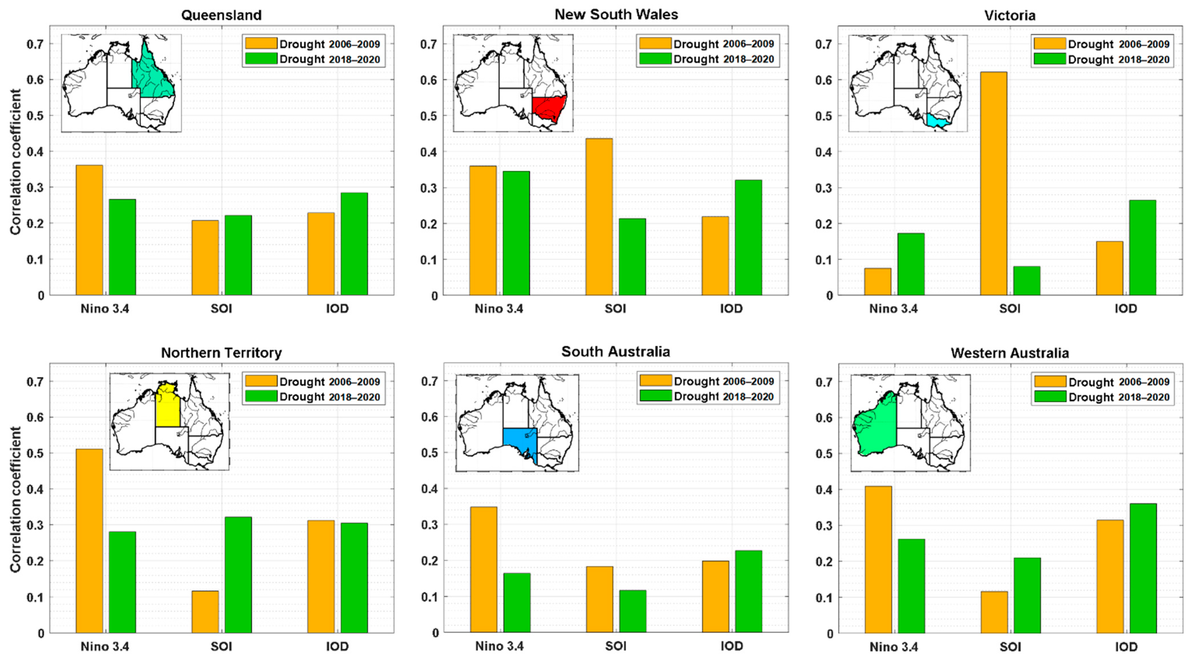
Figure 11.
Spatial distributions of the RMS of residuals in TWSC determined after the removal of all trend and seasonal components.
Figure 11.
Spatial distributions of the RMS of residuals in TWSC determined after the removal of all trend and seasonal components.

Figure 12.
Power spectra of TSDI and Indo-Pacific Climate Variability indices (Nino3.4, SOI and IOD) during (a) Drought 2006–2009; (b) Drought 2018–2020.
Figure 12.
Power spectra of TSDI and Indo-Pacific Climate Variability indices (Nino3.4, SOI and IOD) during (a) Drought 2006–2009; (b) Drought 2018–2020.

Table 1.
Indices used for measuring drought driving factors.
| Index | Detail | Source | Reference |
|---|---|---|---|
| Niño-3.4 | Average SSTs in the Niño-3.4 region (5° S–5° N, 170°–120° W) | https://psl.noaa.gov/gcos_wgsp/Timeseries/Nino34/, accessed on 22 February 2021 | [56] |
| SOI | Atmospheric index calculated using the pressure difference between Tahiti and Darwin | https://psl.noaa.gov/gcos_wgsp/Timeseries/SOI/, accessed on 22 February 2021 | [57,58,59] |
| IOD | Difference in SST anomalies between IOD W (10° S–10° N, 50°–70° E) and IOD E (10° S–10° N, 90°–110° E) | https://psl.noaa.gov/gcos_wgsp/Timeseries/DMI/, accessed on 22 February 2021 | [55] |
Table 2.
Drought grades based on TSDI.
| Drought Grades | Mild | Moderate | Very | Extreme |
|---|---|---|---|---|
| TSDI | 0 to −0.79 | −0.80 to −1.29 | −1.30 to −1.59 | −1.60 and less |
Table 3.
Onset, termination and duration of droughts from April 2002 to May 2020.
| No. | Start Time | Ending Time | Last Time (Months) |
|---|---|---|---|
| 1 | April 2002 | August 2002 | 5 |
| 2 | October 2002 | January 2004 | 16 |
| 3 | October 2004 | March 2006 | 18 |
| 4 * | June 2006 | January 2009 | 32 |
| 5 | March 2009 | May 2010 | 15 |
| 6 | June 2015 | September 2015 | 4 |
| 7 | January 2016 | June 2016 | 6 |
| 8 * | June 2018 | May 2020 | 24 |
(The two longest-lasting droughts are marked with the asterisk).
Table 4.
Maximum drought severity of each region and its corresponding time (unit: cm months).
| Drought Period | Region | Queensland | New South Wales | Victoria | Northern Territory | South Australia | Western Australia |
|---|---|---|---|---|---|---|---|
| Drought 2006–2009 | Maximum Severity | 15.26 | 26.98 | 35.51 | 44.26 | 10.78 | 19.31 |
| Time | January 2007 | June 2007 | June 2007 | December 2008 | February 2007 | January 2009 | |
| Season | Summer | Winter | Winter | Summer | Summer | Summer | |
| Drought 2018–2020 | Maximum Severity | 10.94 | 18.32 | 11.04 | 52.19 | 5.78 | 31.44 |
| Time | January 2020 | February 2020 | March 2019 | January 2020 | February 2020 | May 2020 | |
| Season | Summer | Summer | Autumn | Summer | Summer | Autumn |
Table 5.
The maximum mean absolute correlation coefficients and the lagging times between TSDI and climate indices (Nino3.4, SOI and IOD) for the two droughts (unit of lagging time: months).
Table 5.
The maximum mean absolute correlation coefficients and the lagging times between TSDI and climate indices (Nino3.4, SOI and IOD) for the two droughts (unit of lagging time: months).
| Nino3.4 | SOI | IOD | |
|---|---|---|---|
| Drought 2006–2009 | 0.39/4 | 0.30/0 | 0.27/5 |
| Drought 2018–2020 | 0.26/3 | 0.27/1 | 0.31/6 |
Table 6.
RMS of TWSA for six regions.
| Region | RMS (cm) |
|---|---|
| Queensland | 1.35 |
| New South Wales | 1.21 |
| Victoria | 1.15 |
| Northern Territory | 2.11 |
| South Australia | 0.73 |
| Western Australia | 0.98 |
Publisher’s Note: MDPI stays neutral with regard to jurisdictional claims in published maps and institutional affiliations. |
© 2021 by the authors. Licensee MDPI, Basel, Switzerland. This article is an open access article distributed under the terms and conditions of the Creative Commons Attribution (CC BY) license (https://creativecommons.org/licenses/by/4.0/).
Share and Cite
MDPI and ACS Style
Wang, W.; Shen, Y.; Wang, F.; Li, W. Two Severe Prolonged Hydrological Droughts Analysis over Mainland Australia Using GRACE Satellite Data. Remote Sens. 2021, 13, 1432. https://doi.org/10.3390/rs13081432
AMA Style
Wang W, Shen Y, Wang F, Li W. Two Severe Prolonged Hydrological Droughts Analysis over Mainland Australia Using GRACE Satellite Data. Remote Sensing. 2021; 13(8):1432. https://doi.org/10.3390/rs13081432
Chicago/Turabian StyleWang, Wei, Yunzhong Shen, Fengwei Wang, and Weiwei Li. 2021. "Two Severe Prolonged Hydrological Droughts Analysis over Mainland Australia Using GRACE Satellite Data" Remote Sensing 13, no. 8: 1432. https://doi.org/10.3390/rs13081432
Note that from the first issue of 2016, this journal uses article numbers instead of page numbers. See further details here.