
Toward a Comprehensive Dam Monitoring: On-Site and Remote-Retrieved Forcing Factors and Resulting Displacements (GNSS and PS–InSAR)

 ,
,  ,
,  , and
, and
Abstract
:
1. Introduction
2. Materials and Methods
2.1. Materials
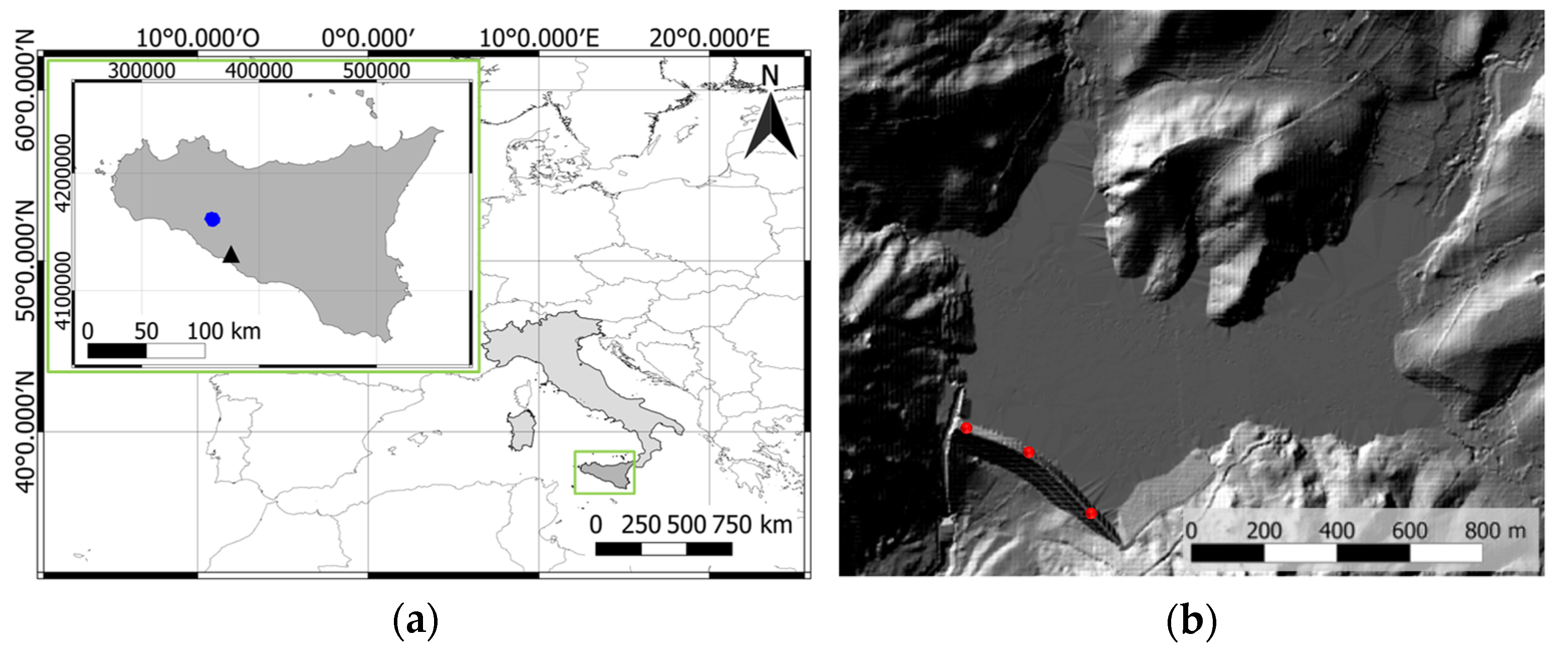
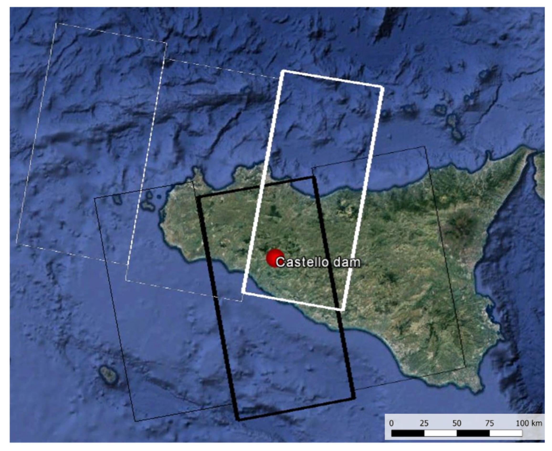
2.1.1. Study Area
2.1.2. Time Series Acquired by Devices Installed In Situ
2.1.3. Remote Time Series Acquisition
2.2. Methods
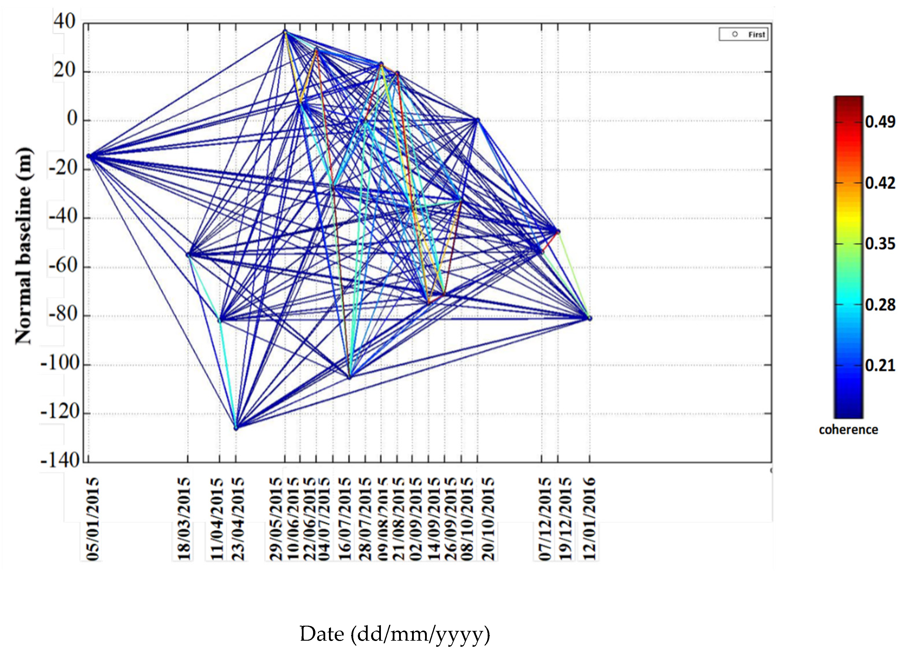
2.2.1. PS–InSAR Displacements
2.2.2. GNSS Displacements
2.2.3. Water Levels
2.2.4. Air and Water Surface Temperatures
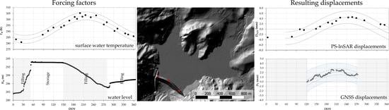
2.2.5. Qualitative–Quantitative Comparisons
3. Results and Discussions
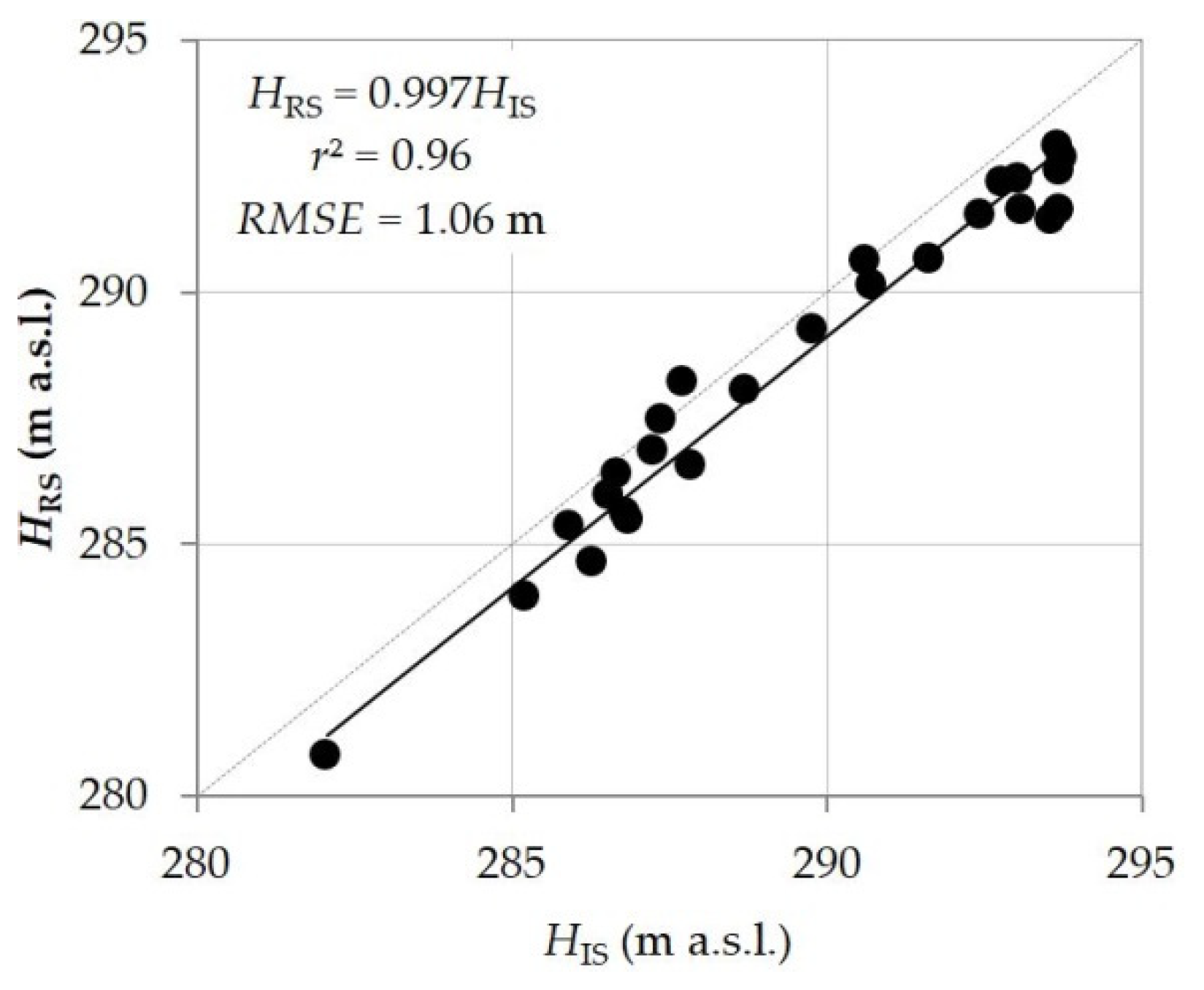
3.1. Water Levels
3.2. Temperatures
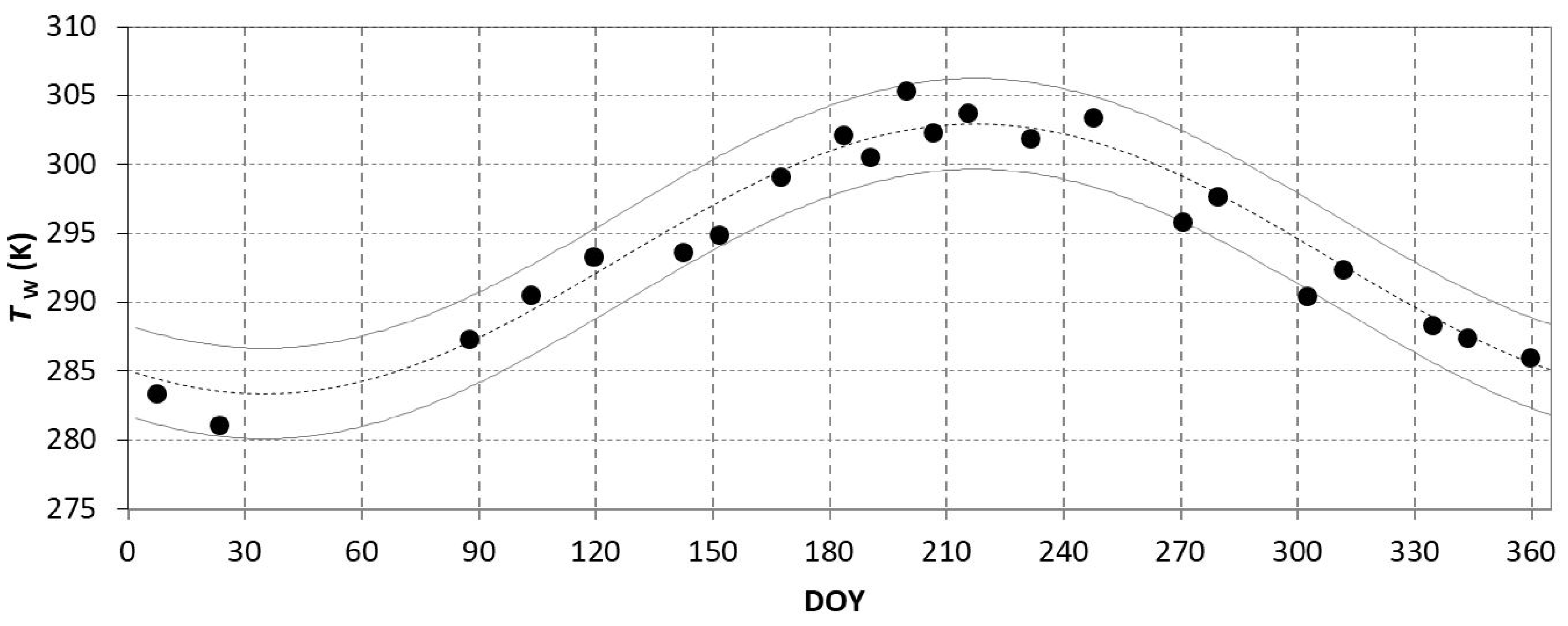
3.2.1. Water Surface Temperature
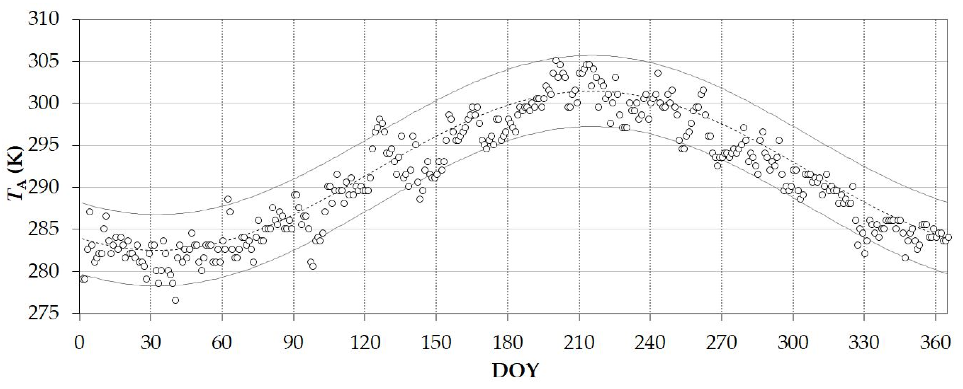
3.2.2. Air Temperature
3.3. Displacements
3.3.1. PS–InSAR Displacements
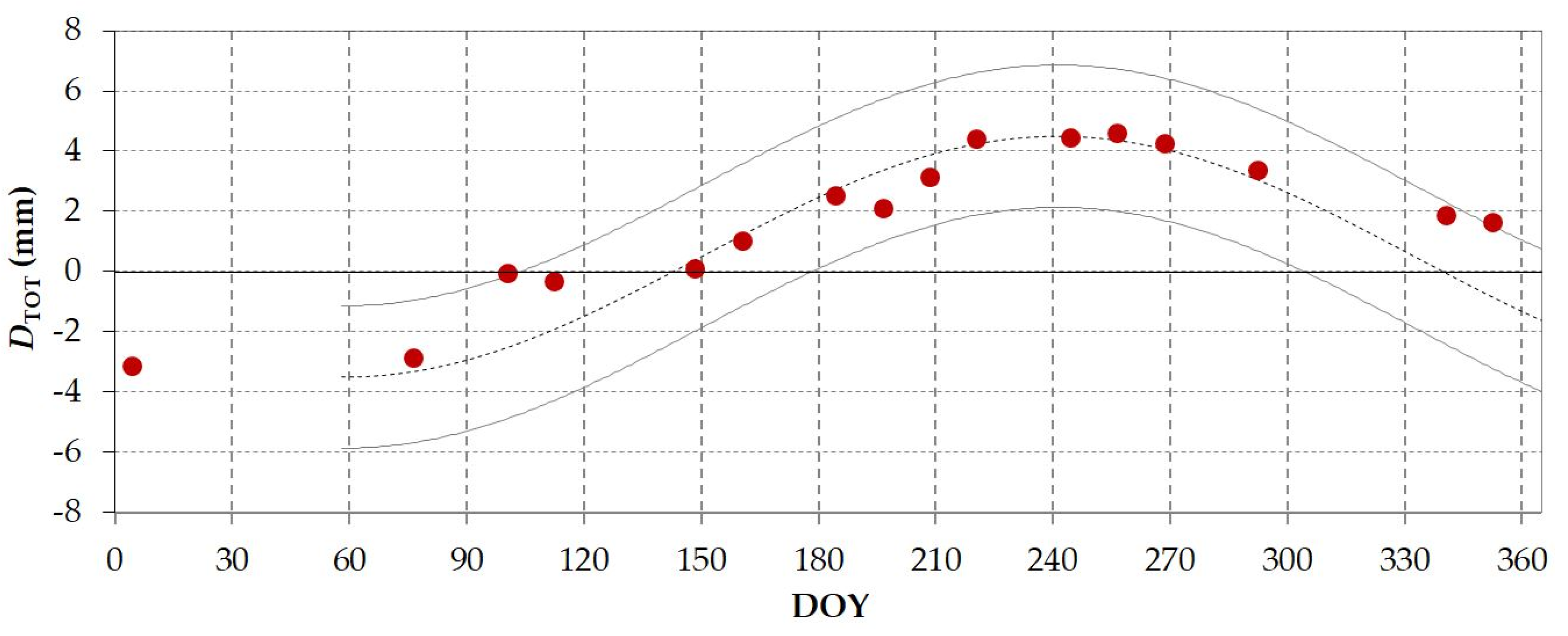
3.3.2. GNSS Displacements
4. Conclusions
Author Contributions
Funding
Institutional Review Board Statement
Informed Consent Statement
Data Availability Statement
Acknowledgments
Conflicts of Interest
Appendix A

| Acronym | Meaning |
|---|---|
| APS | Atmospheric Phase Screen |
| CM-SAF | Climate Monitoring Satellite Application Facility |
| CORS | Continuously Operating Reference Station |
| COSMO-SkyMed | Constellation of Small Satellites for Mediterranean basin Observation |
| DEM | Digital Elevation Model |
| DInSAR | Differential InSAR |
| DOY | Day of Year |
| EPSG | European Petroleum Survey Group |
| ESA | European Space Agency |
| ETRF | European Terrestrial Reference System |
| FEM | Finite Element Method |
| FTP | File Transfer Protocol |
| GACOS | Generic Atmospheric Correction Online Service |
| GNSS | Global Navigation Satellite System |
| ICOLD | International Commission on Large Dams |
| IGS | International GNSS Service |
| InSAR | Interferometric SAR |
| IW | Interferometric Wide |
| IW1, IW2 and IW3 | 1st, 2nd, 3rd IW sub-swath |
| LIDAR | Laser Imaging Detection and Ranging |
| LOS | Line of Sight |
| LST | Land Surface Temperature |
| MBC | Multi-Baseline Construction |
| NDA | Network Deformation Analysis |
| PS | Persistent Scatter |
| PS–InSAR | Persistent Scatter for InSAR |
| QGIS | (until 2013 known as) Quantum GIS |
| RDN2008 | National Dynamic Network, realisation epoch 2008 |
| S-1A, S-1B | Sentinel-1A and Sentinel-1B |
| SAR | Synthetic Aperture Radar |
| SARProZ | The SAR PROcessing tool by periZ |
| SBAS | Small BAseline Subset |
| SLC | Single Look Complex |
| SMW | Statistical Mono-Window |
| SNAP | Sentinel Application Platform software |
| TIRS | Thermal Infrared Sensor |
| TOPSAR | Terrain Observation with Progressive Scans SAR |
| VV | Vertical transmit-Vertical receive polarisation |
| WGS84 | World Geodetic System 1984 |
| Symbol | Meaning | Unit |
|---|---|---|
| σ° | backscattering coefficient | (dB) |
| dLOS | LOS dam displacements | (mm) |
| D | horizontal displacements orthogonal to the dam measured by GNSS | (mm) |
| DTOT | total horizontal displacements orthogonal to the dam | (mm) |
| H | dam water level | (m a.s.l.) |
| HRS | H estimated from remote sensing | (m a.s.l.) |
| HIS | H measured in situ | (m a.s.l.) |
| r2 | determination coefficient | (–) |
| RMSE | Root Mean Square Error | (as the input unit) |
| TA | air temperature | (K) |
| TW | water surface temperature | (K) |
References
- Tomás, R.; Cano, M.; García-Barba, J.; Vicente, F.; Herrera, G.; Lopez-Sanchez, J.M.; Mallorquí, J.J. Monitoring an Earthfill Dam Using Differential SAR Interferometry: La Pedrera Dam, Alicante, Spain. Eng. Geol. 2013, 157, 21–32. [Google Scholar] [CrossRef]
- Al-Husseinawi, Y.; Li, Z.; Clarke, P.; Edwards, S. Evaluation of the Stability of the Darbandikhan Dam after the 12 November 2017 Mw 7.3 Sarpol-e Zahab (Iran-Iraq Border) Earthquake. Remote Sens. 2018, 10, 1426. [Google Scholar] [CrossRef] [Green Version]
- Mazzanti, P.; Perissin, D.; Rocca, A. Structural Health Monitoring of Dams by Advanced Satellite SAR Interferometry: Investigation of Past Processes and Future Monitoring Perspectives. In Proceedings of the 7th Internation Conference on Structural Health Monitoring of Intelligent Infrastructure, Torino, Italy, 1–3 July 2015. [Google Scholar]
- Milillo, P.; Tapete, D.; Cigna, F.; Perissin, D.; Salzer, J.; Lundgren, P.; Fielding, E.; Burgmann, R.; Biondi, F.; Milillo, G.; et al. Structural Health Monitoring of Engineered Structures Using a Space-Borne Synthetic Aperture Radar Multi-Temporal Approach: From Cultural Heritage Sites to War Zones; SPIE: Edinburgh, UK, 2016; Volume 10003. [Google Scholar]
- Milillo, P.; Perissin, D.; Salzer, J.T.; Lundgren, P.; Lacava, G.; Milillo, G.; Serio, C. Monitoring Dam Structural Health from Space: Insights from Novel InSAR Techniques and Multi-Parametric Modeling Applied to the Pertusillo Dam Basilicata, Italy. Int. J. Appl. Earth Obs. Geoinf. 2016, 52, 221–229. [Google Scholar] [CrossRef]
- International Commission on Large Dams. Available online: https://www.icold-cigb.org/ (accessed on 29 March 2021).
- Registro Italiano Dighe—Home Page. Available online: http://dgdighe.mit.gov.it/imagemap/default.htm (accessed on 29 March 2021).
- Osservatorio Delle Acque. Available online: http://www.osservatorioacque.it/?cmd=page&id=dati_monitris_serbatoi&tpl=default (accessed on 29 March 2021).
- Sousa, J.J.; Hlaváčová, I.; Bakoň, M.; Lazecký, M.; Patrício, G.; Guimarães, P.; Ruiz, A.M.; Bastos, L.; Sousa, A.; Bento, R. Potential of Multi-Temporal InSAR Techniques for Bridges and Dams Monitoring. Procedia Technol. 2014, 16, 834–841. [Google Scholar] [CrossRef] [Green Version]
- Scaioni, M.; Marsella, M.; Crosetto, M.; Tornatore, V.; Wang, J. Geodetic and Remote-Sensing Sensors for Dam Deformation Monitoring. Sensors 2018, 18, 3682. [Google Scholar] [CrossRef] [Green Version]
- Kang, F.; Li, J.; Zhao, S.; Wang, Y. Structural Health Monitoring of Concrete Dams Using Long-Term Air Temperature for Thermal Effect Simulation. Eng. Struct. 2019, 180, 642–653. [Google Scholar] [CrossRef]
- Yun, T.; Butler, K.E.; MacQuarrie, K.T.B.; Mclean, B.; Campbell, I. Seasonal Temperature Monitoring and Modelling for Seepage Reconnaissance in an Embankment Dam; European Association of Geoscientists & Engineers: Houten, The Netherlands, 2018. [Google Scholar]
- Yue, H.; Liu, Y. Variations in the Lake Area, Water Level, and Water Volume of Hongjiannao Lake during 1986–2018 Based on Landsat and ASTER GDEM Data. Environ. Monit. Assess. 2019, 191. [Google Scholar] [CrossRef] [PubMed]
- Zhang, R.; Tian, J.; Su, H.; Sun, X.; Chen, S.; Xia, J. Two Improvements of an Operational Two-Layer Model for Terrestrial Surface Heat Flux Retrieval. Sensors 2008, 8, 6165–6187. [Google Scholar] [CrossRef] [PubMed]
- Ma, Y.; Xu, N.; Sun, J.; Wang, X.H.; Yang, F.; Li, S. Estimating Water Levels and Volumes of Lakes Dated Back to the 1980s Using Landsat Imagery and Photon-Counting Lidar Datasets. Remote Sens. Environ. 2019, 232. [Google Scholar] [CrossRef]
- Ferrentino, E.; Nunziata, F.; Buono, A.; Urciuoli, A.; Migliaccio, M. Multipolarization Time Series of Sentinel-1 SAR Imagery to Analyze Variations of Reservoirs’ Water Body. IEEE J. Sel. Top. Appl. Earth Obs. Remote Sens. 2020, 13, 840–846. [Google Scholar] [CrossRef]
- Pipitone, C.; Maltese, A.; Dardanelli, G.; Lo Brutto, M.; La Loggia, G. Monitoring Water Surface and Level of a Reservoir Using Different Remote Sensing Approaches and Comparison with Dam Displacements Evaluated via GNSS. Remote Sens. 2018, 10, 71. [Google Scholar] [CrossRef] [Green Version]
- Droz, P.; Fumagalli, A.; Novali, F.; Young, B. Gps and Insar Technologies: A Joint Approach for the Safety of Lake Sarez. In Proceedings of the 4th Canadian Conference on Geohazards: From Causes to Management, Presse de l’Université Laval, QC, Canada, 23–24 May 2008; pp. 1–8. [Google Scholar]
- Fernandez, J.; Arjona, A.; Prieto, J.F.; Santoyo, M.A.; Seco, A.; Monells, D.; Pallero, J.L.; Prieto, E.; Luzón, F.; Mallorquí, J.J. Study of Surface Displacement Near Itoiz Reservoir, Navarra, Spain, Using an Advanced DInSAR Technique; American Geophysical Union: Washington, DC, USA, 2009. [Google Scholar]
- Grenerczy, G.; Wegmüller, U. Persistent Scatterer Interferometry Analysis of the Embankment Failure of a Red Mud Reservoir Using ENVISAT ASAR Data. Nat. Hazards 2011, 59, 1047–1053. [Google Scholar] [CrossRef]
- Wang, T.; Perissin, D.; Rocca, F.; Liao, M.-S. Three Gorges Dam Stability Monitoring with Time-Series InSAR Image Analysis. Sci. China Earth Sci. 2011, 54, 720–732. [Google Scholar] [CrossRef]
- Voege, M.; Frauenfelder, R.; Larsen, Y. Displacement Monitoring at Svartevatn Dam with Interferometric SAR. In Proceedings of the 2012 IEEE International Geoscience and Remote Sensing Symposium, Munich, Germany, 22–27 July 2012; pp. 3895–3898. [Google Scholar]
- Awada, H.; Ciraolo, G.; Maltese, A.; Provenzano, G.; Moreno Hidalgo, M.A.; Còrcoles, J.I. Assessing the Performance of a Large-Scale Irrigation System by Estimations of Actual Evapotranspiration Obtained by Landsat Satellite Images Resampled with Cubic Convolution. Int. J. Appl. Earth Obs. Geoinf. 2019, 75, 96–105. [Google Scholar] [CrossRef]
- Sharaf, N.; Fadel, A.; Bresciani, M.; Giardino, C.; Lemaire, B.J.; Slim, K.; Faour, G.; Vinçon-Leite, B. Lake Surface Temperature Retrieval from Landsat-8 and Retrospective Analysis in Karaoun Reservoir, Lebanon. J. Appl. Rem. Sens. 2019, 13, 044505. [Google Scholar] [CrossRef]
- Addesso, P.; Longo, M.; Maltese, A.; Montone, R.; Restaino, R.; Vivone, G. Robustified Smoothing for Enhancement of Thermal Image Sequences Affected by Clouds. In Proceedings of the 2015 IEEE International Geoscience and Remote Sensing Symposium (IGARSS), Milan, Italy, 26–31 July 2015; pp. 1076–1079. [Google Scholar]
- Addesso, P.; Longo, M.; Restaino, R.; Vivone, G. Spatio-Temporal Resolution Enhancement for Cloudy Thermal Sequences. Eur. J. Remote Sens. 2019, 52, 2–14. [Google Scholar] [CrossRef] [Green Version]
- Barzaghi, R.; Cazzaniga, N.E.; De Gaetani, C.I.; Pinto, L.; Tornatore, V. Estimating and Comparing Dam Deformation Using Classical and Gnss Techniques. Sensors 2018, 18, 756. [Google Scholar] [CrossRef] [PubMed] [Green Version]
- De Sortis, A.; Paoliani, P. Statistical Analysis and Structural Identification in Concrete Dam Monitoring. Eng. Struct. 2007, 29, 110–120. [Google Scholar] [CrossRef]
- Di Martire, D.; Iglesias, R.; Monells, D.; Centolanza, G.; Sica, S.; Ramondini, M.; Pagano, L.; Mallorquí, J.J.; Calcaterra, D. Comparison between Differential SAR Interferometry and Ground Measurements Data in the Displacement Monitoring of the Earth-Dam of Conza Della Campania (Italy). Remote Sens. Environ. 2014, 148, 58–69. [Google Scholar] [CrossRef]
- Blanco-Sánchez, P.; Mallorquí, J.J.; Duque, S.; Monells, D. The Coherent Pixels Technique (CPT): An Advanced DInSAR Technique for Nonlinear Deformation Monitoring. Pure Appl. Geophys. 2008, 165, 1167–1193. [Google Scholar] [CrossRef]
- Xiao, R.; Shi, H.; He, X.; Li, Z.; Jia, D.; Yang, Z. Deformation Monitoring of Reservoir Dams Using GNSS: An Application to South-to-North Water Diversion Project, China. IEEE Access 2019, 7, 54981–54992. [Google Scholar] [CrossRef]
- Empson, W.; Cohen, D.; Gamm, S.; Worsham, B.; Yarborough, S. Karst Investigation Program Guided by Synthetic Aperture Radar. In Proceedings of the Remote Sensing for Agriculture, Ecosystems, and Hydrology XXI; Neale, C.M., Maltese, A., Eds.; SPIE: Strasbourg, France, 2019; p. 42. [Google Scholar]
- Lazecký, M.; Perissin, D.; Zhiying, W.; Ling, L.; Yuxiao, Q. Observing dam’s movements with spaceborne sar interferometry. In Engineering Geology for Society and Territory—Volume 5: Urban Geology, Sustainable Planning and Landscape Exploitation; Springer: Berlin/Heidelberg, Germany, 2015; pp. 131–136. [Google Scholar]
- Milillo, P.; Porcu, M.C.; Lundgren, P.; Soccodato, F.; Salzer, J.; Fielding, E.; Burgmann, R.; Milillo, G.; Perissin, D.; Biondi, F. The Ongoing Destabilization of the Mosul Dam as Observed by Synthetic Aperture Radar Interferometry. In Proceedings of the 2017 IEEE International Geoscience and Remote Sensing Symposium (IGARSS), Fort Worth, TX, USA, 23–28 July 2017; pp. 6279–6282. [Google Scholar]
- Milillo, P.; Bürgmann, R.; Lundgren, P.; Salzer, J.; Perissin, D.; Fielding, E.; Biondi, F.; Milillo, G. Space Geodetic Monitoring of Engineered Structures: The Ongoing Destabilization of the Mosul Dam, Iraq. Sci. Rep. 2016, 6. [Google Scholar] [CrossRef] [Green Version]
- Bakon, M.; Perissin, D.; Lazecky, M.; Papco, J. Infrastructure Non-Linear Deformation Monitoring Via Satellite Radar Interferometry. Procedia Technol. 2014, 16, 294–300. [Google Scholar] [CrossRef] [Green Version]
- Ferretti, A.; Prati, C.; Rocca, F. Permanent Scatterers in SAR Interferometry. IEEE Trans. Geosci. Remote Sens. 2001, 39, 8–20. [Google Scholar] [CrossRef]
- Crosetto, M.; Monserrat, O.; Cuevas-González, M.; Devanthéry, N.; Crippa, B. Persistent Scatterer Interferometry: A Review. ISPRS J. Photogramm. Remote Sens. 2016, 115, 78–89. [Google Scholar] [CrossRef] [Green Version]
- Ruiz-Armenteros, A.M.; Lazecky, M.; Hlaváčová, I.; Bakoň, M.; Manuel Delgado, J.; Sousa, J.J.; Lamas-Fernández, F.; Marchamalo, M.; Caro-Cuenca, M.; Papco, J.; et al. Deformation Monitoring of Dam Infrastructures via Spaceborne MT-InSAR. The Case of La Viñuela (Málaga, Southern Spain). Procedia Comput. Sci. 2018, 138, 346–353. [Google Scholar] [CrossRef]
- Berardino, P.; Fornaro, G.; Lanari, R.; Sansosti, E. A New Algorithm for Surface Deformation Monitoring Based on Small Baseline Differential SAR Interferograms. IEEE Trans. Geosci. Remote Sens. 2002, 40, 2375–2383. [Google Scholar] [CrossRef] [Green Version]
- Bonano, M.; Manunta, M.; Marsella, M.; Lanari, R. Long-Term ERS/ENVISAT Deformation Time-Series Generation at Full Spatial Resolution via the Extended SBAS Technique. Int. J. Remote Sens. 2012, 33, 4756–4783. [Google Scholar] [CrossRef]
- Corsetti, M.; Manunta, M.; Marsella, M.; Scifoni, S.; Sonnessa, A.; Ojha, C. Satellite techniques: New perspectives for the monitoring of dams. In Engineering Geology for Society and Territory—Volume 5: Urban Geology, Sustainable Planning and Landscape Exploitation; Springer: Berlin/Heidelberg, Germany, 2015; pp. 989–993. [Google Scholar]
- Mura, J.C.; Gama, F.F.; Paradella, W.R.; Negrão, P.; Carneiro, S.; de Oliveira, C.G.; Brandão, W.S. Monitoring the Vulnerability of the Dam and Dikes in Germano Iron Mining Area after the Collapse of the Tailings Dam of Fundão (Mariana-MG, Brazil) Using DInSAR Techniques with TerraSAR-X Data. Remote Sens. 2018, 10, 1507. [Google Scholar] [CrossRef] [Green Version]
- Li, F.K.; Goldstein, R.M. Studies of Multibaseline Spaceborne Interferometric Synthetic Aperture Radars. IEEE Trans. Geosci. Remote Sens. 1990, 28, 88–97. [Google Scholar] [CrossRef]
- Zebker, H.A.; Villasenor, J. Decorrelation in Interferometric Radar Echoes. IEEE Trans. Geosci. Remote Sens. 1992, 30, 950–959. [Google Scholar] [CrossRef] [Green Version]
- Copernicus Sentinels POD Data Hub. Available online: https://scihub.copernicus.eu/gnss/#/home (accessed on 29 March 2021).
- Reigber, C.; Xia, Y.; Kaufmann, H.; Massmann, F.-H.; Timmen, L.; Bodechtel, J.; Frei, M. Fringe 96 Workshop on ERS SAR Interferometry. In Proceedings of the Fringe 96 Workshop, Zurich, Switzerland, 30 September–2 October 1996. [Google Scholar]
- Dardanelli, G.; La Loggia, G.; Perfetti, N.; Capodici, F.; Puccio, L.; Maltese, A. Monitoring Displacements of an Earthen Dam Using GNSS and Remote Sensing; SPIE: Amsterdam, The Netherlands, 2014; Volume 9239. [Google Scholar]
- Szostak-Chrzanowski, A.; Chrzanowski, A.; Massiéra, M. Use of Deformation Monitoring Results in Solving Geomechanical Problems—Case Studies. Eng. Geol. 2005, 79, 3–12. [Google Scholar] [CrossRef]
- Dardanelli, G.; Pipitone, C. Hydraulic Models and Finite Elements for Monitoring of an Earth Dam, by Using GNSS Techniques. Period. Polytech. Civ. Eng. 2016. [Google Scholar] [CrossRef] [Green Version]
- Copernicus Open Access Hub. Available online: https://scihub.copernicus.eu/dhus/#/home (accessed on 29 March 2021).
- Bovenga, F.; Wasowski, J.; Nitti, D.O.; Nutricato, R.; Chiaradia, M.T. Using COSMO/SkyMed X-Band and ENVISAT C-Band SAR Interferometry for Landslides Analysis. Remote Sens. Environ. 2012, 119, 272–285. [Google Scholar] [CrossRef]
- Perissin, Daniele Software Manual—SARPROZ©. Available online: https://www.sarproz.com/software-manual/ (accessed on 29 March 2021).
- Pipitone, C.; Maltese, A.; Dardanelli, G.G.; Capodici, F.; Lo Brutto, M.; La Loggia, G. Detection of a Reservoir Water Level Using Shape Similarity Metrics. In Remote Sensing for Agriculture, Ecosystems, and Hydrology XIX; Neale, C.M., Maltese, A., Eds.; SPIE: Warsaw, Poland, 2017; p. 61. [Google Scholar]
- Goldstein, R.M.; Werner, C.L. Radar Interferogram Filtering for Geophysical Applications. Geophys. Res. Lett. 1998, 25, 4035–4038. [Google Scholar] [CrossRef] [Green Version]
- Pipitone, C.; Cigna, F.; Dardanelli, G.; La Loggia, G.; Maltese, A.; Muller, J.-P. Reservoir Monitoring Using Satellite SAR and GNSS: A Case Study in Southern Italy. EPIC Ser. Eng. 2018, 3, 1682–1691. [Google Scholar]
- De Zan, F.; Guarnieri, A.M. TOPSAR: Terrain Observation by Progressive Scans. IEEE Trans. Geosci. Remote Sens. 2006, 44, 2352–2360. [Google Scholar] [CrossRef]
- Yu, C.; Li, Z.; Penna, N.T. Generic Atmospheric Correction Online Service for InSAR (GACOS): Validation and Implications for InSAR Time Series Analysis; American Geophysical Union: Washington, DC, USA, 2018; Volume 32. [Google Scholar]
- Yu, C.; Li, Z.; Penna, N.T. Interferometric Synthetic Aperture Radar Atmospheric Correction Using a GPS-Based Iterative Tropospheric Decomposition Model. Remote Sens. Environ. 2018, 204, 109–121. [Google Scholar] [CrossRef]
- Yu, C.; Penna, N.T.; Li, Z. Generation of Real-Time Mode High-Resolution Water Vapor Fields from GPS Observations. J. Geophys. Res. Atmos. 2017, 122, 2008–2025. [Google Scholar] [CrossRef]
- Yu, C.; Li, Z.; Penna, N.T. Triggered Afterslip on the Southern Hikurangi Subduction Interface Following the 2016 Kaikōura Earthquake from InSAR Time Series with Atmospheric Corrections. Remote Sens. Environ. 2020, 251, 112097. [Google Scholar] [CrossRef]
- Generic Atmospheric Correction Online Service for InSAR (GACOS). Available online: http://www.gacos.net/ (accessed on 29 March 2021).
- Piano Assetto Idrogeologico, Sistema Informativo Territoriale Regionale. Available online: https://www.sitr.regione.sicilia.it/pai-download-dati (accessed on 29 March 2021).
- Perissin, D.; Wang, Z.; Wang, T. The SARPROZ InSAR Tool for Urban Subsidence/Manmade Structure Stability Monitoring in China. In Proceedings of the ISRSE, Sidney, Australia, 10–15 April 2011; pp. 1–4. [Google Scholar]
- Eriksen, H.Ø.; Lauknes, T.R.; Larsen, Y.; Corner, G.D.; Bergh, S.G.; Dehls, J.; Kierulf, H.P. Visualizing and Interpreting Surface Displacement Patterns on Unstable Slopes Using Multi-Geometry Satellite SAR Interferometry (2D InSAR). Remote Sens. Environ. 2017, 191, 297–312. [Google Scholar] [CrossRef] [Green Version]
- Hu, J.; Li, Z.W.; Ding, X.L.; Zhu, J.J.; Zhang, L.; Sun, Q. Resolving Three-Dimensional Surface Displacements from InSAR Measurements: A Review. Earth Sci. Rev. 2014, 133, 1–17. [Google Scholar] [CrossRef]
- Saastamoinen, J. Atmospheric Correction for the Troposphere and Stratosphere in Radio Ranging Satellites. In The Use of Artificial Satellites for Geodesy; American Geophysical Union (AGU): Washington, DC, USA, 1972; pp. 247–251. ISBN 978-1-118-66364-6. [Google Scholar]
- Niell, A.E. Global Mapping Functions for the Atmosphere Delay at Radio Wavelengths. J. Geophys. Res. Solid Earth 1996, 101, 3227–3246. [Google Scholar] [CrossRef]
- Klobuchar, J.A. Ionospheric Effects on GPS. In Global Positioning System: Theory and Application; Aeronautics and Astronautics: Stanford, CA, USA, 1996. [Google Scholar]
- Schwiderski, E.W. On Charting Global Ocean Tides. Rev. Geophys. 1980, 18, 243–268. [Google Scholar] [CrossRef]
- Teunissen, P.J.G. The Least-Squares Ambiguity Decorrelation Adjustment: A Method for Fast GPS Integer Ambiguity Estimation. J. Geod. 1995, 70, 65–82. [Google Scholar] [CrossRef]
- Small, D.; Schubert, A. Guide to ASAR Geocoding. ESA-ESRIN Tech. Note RSL-ASAR-GC-AD 2008, 1, 36. [Google Scholar]
- Vickers, H.; Malnes, E.; Høgda, K.-A. Long-Term Water Surface Area Monitoring and Derived Water Level Using Synthetic Aperture Radar (SAR) at Altevatn, a Medium-Sized Arctic Lake. Remote Sens. 2019, 11, 2780. [Google Scholar] [CrossRef] [Green Version]
- QGIS. A Free and Open Source Geographic Information System. Available online: https://qgis.org/en/site/ (accessed on 29 March 2021).
- Ji, S.; Zhu, Y.; Qiang, S.; Zeng, D. Forecast of Water Temperature in Reservoir Based on Analytical Solution. J. Hydrodyn. Ser. B 2008, 20, 507–513. [Google Scholar] [CrossRef]
- Duguay-Tetzlaff, A.; Bento, V.A.; Göttsche, F.M.; Stöckli, R.; Martins, J.P.A.; Trigo, I.; Olesen, F.; Bojanowski, J.S.; da Camara, C.; Kunz, H. Meteosat Land Surface Temperature Climate Data Record: Achievable Accuracy and Potential Uncertainties. Remote Sens. 2015, 7, 13139–13156. [Google Scholar] [CrossRef] [Green Version]
- Ermida, S.L.; Soares, P.; Mantas, V.; Göttsche, F.-M.; Trigo, I.F. Google Earth Engine Open-Source Code for Land Surface Temperature Estimation from the Landsat Series. Remote Sens. 2020, 12, 1471. [Google Scholar] [CrossRef]
- Piccolroaz, S. Prediction of Lake Surface Temperature Using the Air2water Model: Guidelines, Challenges, and Future Perspectives. Adv. Oceanogr. Limnol. 2016, 7, 36–50. [Google Scholar] [CrossRef] [Green Version]
- Osmanoğlu, B.; Sunar, F.; Wdowinski, S.; Cabral-Cano, E. Time Series Analysis of InSAR Data: Methods and Trends. ISPRS J. Photogramm. Remote Sens. 2016, 115, 90–102. [Google Scholar] [CrossRef]
- Geoportale Nazionale. Available online: http://www.pcn.minambiente.it/mattm/servizio-wms/ (accessed on 29 March 2021).
- Farquharson, G.; Woods, W.; Stringham, C.; Sankarambadi, N.; Riggi, L. The Capella Synthetic Aperture Radar Constellation. In Proceedings of the IGARSS 2018–2018 IEEE International Geoscience and Remote Sensing Symposium, Aachen, Germany, 4–7 June 2018; pp. 1873–1876. [Google Scholar]


| Period 1 | Period 2 | Period 3 | Period 4 | ||||
|---|---|---|---|---|---|---|---|
| Filling | Storing | Emptying | Filling | ||||
| ascending | descending | ascending | descending | ascending | descending | ascending | descending |
| 05/01/15 | 12/03/15 | 23/05/15 | 20/10/15 | ||||
| 11/01/15 | 18/03/15 | 04/06/15 | 07/12/15 | ||||
| 28/02/15 | 24/03/15 | 10/06/15 | 19/11/15 | ||||
| 05/04/15 | 22/06/15 | 13/12/15 | |||||
| 11/04/15 | 04/07/15 | 19/12/15 | |||||
| 17/04/15 | 10/07/15 | 25/12/15 | |||||
| 23/04/15 | 16/07/15 | 12/01/16 | |||||
| 29/04/15 | 22/07/15 | ||||||
| 11/05/15 | 28/07/15 | ||||||
| 29/05/15 | 09/08/15 | ||||||
| 21/08/15 | |||||||
| 27/08/15 | |||||||
| 02/09/15 | |||||||
| 08/09/15 | |||||||
| 14/09/15 | |||||||
| 26/09/15 | |||||||
| 08/10/15 | |||||||
Publisher’s Note: MDPI stays neutral with regard to jurisdictional claims in published maps and institutional affiliations. |
© 2021 by the authors. Licensee MDPI, Basel, Switzerland. This article is an open access article distributed under the terms and conditions of the Creative Commons Attribution (CC BY) license (https://creativecommons.org/licenses/by/4.0/).
Share and Cite
Maltese, A.; Pipitone, C.; Dardanelli, G.; Capodici, F.; Muller, J.-P. Toward a Comprehensive Dam Monitoring: On-Site and Remote-Retrieved Forcing Factors and Resulting Displacements (GNSS and PS–InSAR). Remote Sens. 2021, 13, 1543. https://doi.org/10.3390/rs13081543
Maltese A, Pipitone C, Dardanelli G, Capodici F, Muller J-P. Toward a Comprehensive Dam Monitoring: On-Site and Remote-Retrieved Forcing Factors and Resulting Displacements (GNSS and PS–InSAR). Remote Sensing. 2021; 13(8):1543. https://doi.org/10.3390/rs13081543
Chicago/Turabian StyleMaltese, Antonino, Claudia Pipitone, Gino Dardanelli, Fulvio Capodici, and Jan-Peter Muller. 2021. "Toward a Comprehensive Dam Monitoring: On-Site and Remote-Retrieved Forcing Factors and Resulting Displacements (GNSS and PS–InSAR)" Remote Sensing 13, no. 8: 1543. https://doi.org/10.3390/rs13081543