Simultaneous Identification of Bridge Structural Damage and Moving Loads Using the Explicit Form of Newmark-β Method: Numerical and Experimental Studies

Abstract

Bridge infrastructures are always subjected to degradation because of aging, their environment, and excess loading. Now it has become a worldwide concern that a large proportion of bridge infrastructures require significant maintenance. This compels the engineering community to develop a robust method for condition assessment of the bridge structures. Here, the simultaneous identification of moving loads and structural damage based on the explicit form of the Newmark-β method is proposed. Although there is an extensive attempt to identify moving loads with known structural parameters, or vice versa, their simultaneous identification considering the road roughness has not been studied enough. Furthermore, most of the existing time domain methods are developed for structures under non-moving loads and are commonly formulated by state-space method, thus suffering from the errors of discretization and sampling ratio. This research is believed to be among the few studies on condition assessment of bridge structures under moving vehicles considering factors such as sensor placement, sampling frequency, damage type, measurement noise, vehicle speed, and road surface roughness with numerical and experimental verifications. Results indicate that the method is able to detect damage with at least three sensors, and is not sensitive to sensors location, vehicle speed and road roughness level. Current limitations of the study as well as prospective research developments are discussed in the conclusion.

1. Introduction

Moving load-based damage detection methods have attracted significant attention recently, as they have several advantages over other damage detection methods, such as [1,2,3,4,5,6,7,8,9,10]:

(1)

There are no traffic interruptions;

(2)

Analysis is performed under operational environment conditions;

(3)

Analysis is performed continuously;

(4)

There is no need for exceptional experimental arrangements or techniques;

(5)

The number of sensors and amount of expense is reduced;

(6)

There is the ability for excitation of structural vibrations with a large amplitude and high signal-to-noise ratio.

The dynamic interaction force between vehicles and road surface can be intensified by structural damage, road surface roughness and vehicle speed. Therefore, it is of high importance to simultaneously identify moving loads and structural damage while considering road surface roughness. Although there have been extensive attempts to identify moving loads with known structural parameters [11,12,13,14,15,16], or to identify structural parameters subject to non-moving loads, moving masses or knowing moving loads, their simultaneous identification has not been studied enough [17,18,19,20,21,22].

In reality, unknown damages and unknown moving loads can exist together, influencing the response of the system. To address this problem, different algorithms have been developed using output only. Hoshiya and Maruyama [23] applied a weighted global iteration procedure to simultaneously identify moving loads and modal parameters of a simply supported beam. Extended Kalman filter was used in their method.

Zhu and Law [24] presented a method based on displacement measurements to simultaneously identify moving loads and crack damage. They verified the method numerically for a simply supported beam considering measurement noise, road roughness, and the number of beam elements in the finite element model. Results showed that the method is sensitive to road roughness. This method has not been verified for a multiple span bridge or experimentally, and it requires a full-sensor placement. This method later was extended by Law and Li [25] and numerically verified by a three-span pre-stressed concrete box-section bridge under the action of a two-axle three-dimensional vehicle. The results of this comprehensive study have indicated that a sufficient number of sensors are needed, and that the accuracy of identified moving loads can greatly affect the accuracy of damage detection.

Lu and Law [17] proposed a method based on the sensitivity of dynamic response to simultaneously identify moving loads and damage. Sinusoidal and impulsive forces with known locations were studied. The method was verified numerically by a single-span simply supported bean and a two-span continuous concrete beam as well as experimentally by a simply supported steel beam. Numerical results show no false alarm in any other adjacent undamaged elements, however, in experimental results there was considerable false identification of damage in adjacent elements. Zhang et al. [18,19] presented a method based on the Virtual Distortion Method for simultaneous identification of moving mass and structural damage. In this method a couple of masses are moving on a flat bridge at constant speeds. In these studies, the vehicle model is not considered as an excitation source and the effect of road surface roughness is not considered.

Later, Zhang et al. [26] presented a method for simultaneous identification of moving vehicles and bridge damage considering road surface roughness. In this study, the vehicle parameters and structural damage were treated as optimization variables. The method was numerically verified by a 200 m long three-span bridge, and the robustness of the method for model error and measurement noise was tested. However, the effects of different uncertainties such as different levels of road roughness, vehicle speed, damage location and extension, as well as computation time were not discussed.

Sun and Betti [21] presented a hybrid artificial bee colony strategy to simultaneously identify structural parameters and, when possible, dynamic input time histories from incomplete sets of acceleration measurements. The method has been numerically verified by three types of frames. In this method, the non-moving load is considered as an excitation source, and it is highly sensitive to measurement noise.

Feng et al. [27] proposed a method of utilizing a limited number of sensors to simultaneously identify bridge structural parameters and vehicle axle loads via an iterative parametric optimization process. The study applied a Bayesian inference-based regularization approach in an attempt to solve the ill-posed least squares problem for the unknown vehicle axle loads. Yet while this method was numerically verified over different vehicle speeds and levels of noise, both for a simply supported bridge and a three-span continuous bridge, the effect of roughness was not directly considered, and the method showed load identification errors over mid supports.

Abbasnia et al. [28] developed a sensitivity-based damage detection method referred to as Adjoint Variable Method (AVM) to simultaneously identify moving loads and structural damage. The effectiveness of the proposed method is numerically illustrated by a two-span continuous girder and a plate. The method is sensitive to noise greater than 1.4% and the effect of road roughness is not explored. Obrien et al. [29] proposed a method for damage detection based on moving force identification. A two-dimensional vehicle-bridge interaction model is used for numerical verification. Both strains and deflections have been studied as measured responses. Results indicate that strain measurements are effective only when the sensor is close to the damage zone. Furthermore, the method is sensitive to damage location, and it can be identified well only if it is close to the center of the beam.

Jayalakshmi et al. [22] presented an approach to simultaneously identify structural parameters and non-moving dynamic forces and verified them numerically by use of three examples of a simply supported beam, a building, and a truss bridge. This approach is based on a newly developed dynamic hybrid adaptive firefly algorithm (DHAFA) and a modified version of Tikhonov regularization plus the explicit form of the Newmark-β method. There are many limitations to reaching acceptable results by this method such as:

(1)

Sensors should be available at the location of dynamic forces,

(2)

One input force-time history should be known,

(3)

The known load should be in the range of 0.6 times to 1.5 times of the unknown forces. In practice however, these assumptions are not so simple to apply. Wang et al. [30] developed a method for simultaneous identification of the load and unknown parameters where the excitation source is non-moving.

Most of the studies of simultaneous identification of damage and load are for non-moving loads, and those which are for structures under moving loads are not investigated comprehensively for different uncertainties or are not verified experimentally. Furthermore, moving load identification in existing studies is commonly formulated in state space, which is sensitive to discretization and sampling rate [11,12,13,14,15,16]. Liu et al. [31] developed and verified the explicit form of the Newmark-β method for a force identification of a full structure under a non-moving load. It is shown to be superior to the state space method. Later, the authors of this paper developed the method for moving load identification for bridge structures and verified the results numerically and experimentally, which are published in the reference [32].

This project is believed to be among the few studies on simultaneous identification of moving load and structural damage considering factors such as measurement noise, road surface roughness, sampling frequency, sensor placement, number of spans, number of elements in the finite element model of the bridge, and the vehicle speed. Furthermore, results are verified by numerical and experimental studies. In this study, strain and acceleration measurements are used as inputs. There is no need for complete measurements at interface nodes as well as no need for interface force measurements. The moving vehicle is unknown and only its location and speed is needed to be known in advance.

In this Paper, a review of dynamics of the vehicle-bridge interaction system and moving load identification based on the explicit form of Newmark-β method is presented in Section 2 and Section 3, in order. Section 4 describes the element damage index, sensitivities of dynamic responses, and how it can be used to detect damage. The iterative identification procedure to simultaneously identify moving loads and structural parameters is also described in this section. In Section 5, the numerical analyses of a single-span simply supported bridge is conducted to demonstrate the accuracy and efficiency of the proposed method. The effects of measurement noise, sensor placement, damage location and extension, vehicle speed, and road surface roughness on the accuracy of the method are investigated. In Section 6, a two-span continuous bridge is studied to check if mid-supports affect the accuracy of the method. 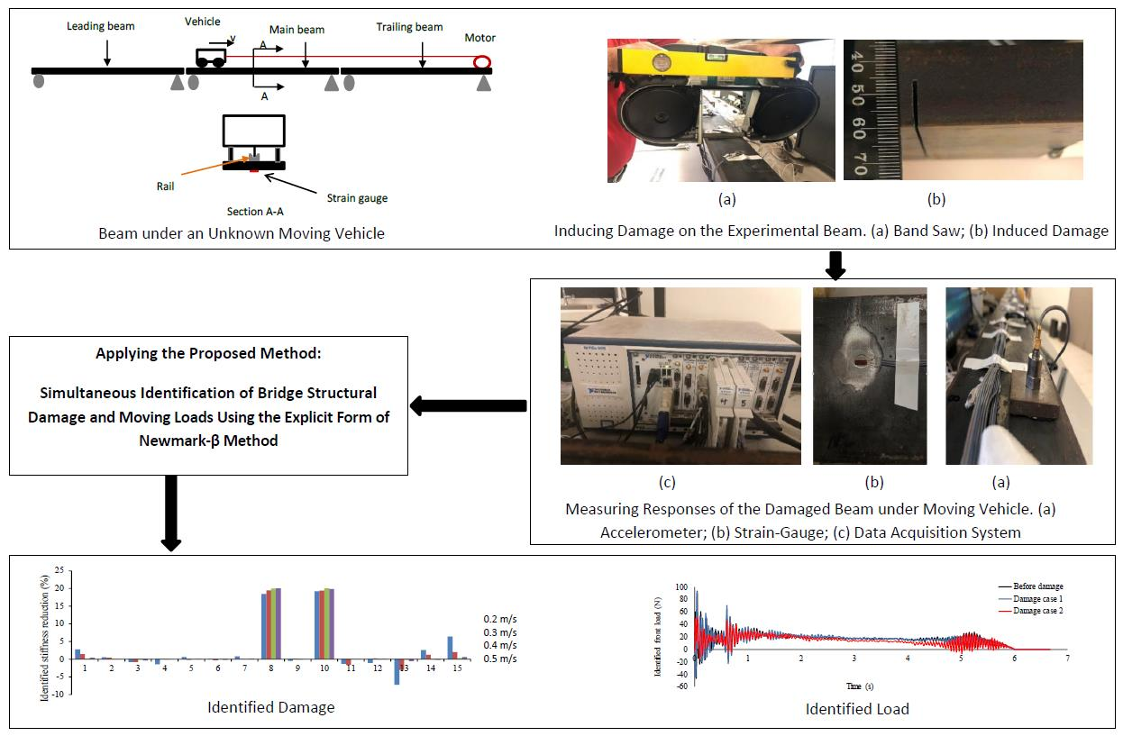Section 7, delivers an experimental study in the laboratory to verify the proposed techniques experimentally. The set up mainly includes a 3 m single-span simply supported beam excited by a four-wheel car being pulled through the beam by an electronic motor. The advantages and limitations of the proposed method are summarized in Section 8.

2. Dynamics of the Vehicle-Bridge Interaction System

2.1. Bridge Model

The equation of motion of the bridge subjected to a moving vehicle can be written as:

$${\mathit{M}}_B{\ddot{\mathit{y}}}_B+{\mathit{C}}_B{\dot{\mathit{y}}}_B+{\mathit{K}}_B{\mathit{y}}_B={\mathit{N}}_b{\mathit{F}}_{int}$$

(1)

where ${\mathit{M}}_B$, C_B and ${\mathit{K}}_B$ are the bridge mass, damping, and stiffness matrices, respectively;${\mathit{y}}_B$, ${\dot{\mathit{y}}}_B$, and ${\ddot{\mathit{y}}}_B$ are the nodal displacement, velocity, and acceleration vectors, respectively. The beam is discretized into $n_{el}$ equally spaced elements with $n_{el}+1$ nodes. Each node includes two degrees of freedom (DOFs), rotational and vertical translations. The total number of DOFs for the bridge is $ndof=2\times \left(n_{el}+1\right)$.

The half vehicle model with two axles is used in this study and ${\left({\mathit{N}}_b{\mathit{F}}_{int}\right)}_{ndof\times 1}$ is an equivalent global load vector at each time instant. The matrix ${\mathit{N}}_b$ is a $ndof\times 2$ transformation matrix that distributes interaction forces (${\mathit{F}}_{int}$) to equivalent nodal forces, which consists of the Hermitian shape function vectors at the DOFs of the beam elements where interaction forces are acting and zeros for the other entries. More details in this regard can be found in reference [32].

2.2. Vehicle Model and Vehicle-Bridge Coupled Model

To apply the proposed method in reality, only the location and speed of the vehicle is needed to be known in advance. However, to simulate the bridge responses in numerical studies, a half-car model with four degrees of freedom is used and a vehicle-bridge model is developed.

Road surface roughness distinctly affects the dynamic responses of both the bridge and vehicles. The ISO 8608 classifies road profiles from A (very good) to H (very poor) according to their degree of roughness. In this study, the effects of road roughness at levels A (very good), B (good), and C (average) are considered to simulate bridge responses for numerical study. To find out how the road roughness is simulated, refer to reference [32].

3. Moving Load Identification Formula Based on the Explicit Form of Newmark-β Method

The authors of this paper previously developed the explicit form of Newmark-β method to identify moving loads on an intact bridge structure [32]. As a result of the developed method, Equation (1) can be represented as below:

$$\left[\begin{array}{c}{\mathit{y}}_{t=i}\\ {\dot{\mathit{y}}}_{t=i}\\ {\ddot{\mathit{y}}}_{t=i}\end{array}\right]={\displaystyle \sum _{j=0}^{i-1}}{\left[\begin{array}{c}{\mathit{A}}_d{\mathit{A}}_v{\mathit{A}}_a\\ {\mathit{B}}_d{\mathit{B}}_v{\mathit{B}}_a\\ {\mathit{C}}_d{\mathit{C}}_v{\mathit{C}}_a\end{array}\right]}^j\left[\begin{array}{c}{\mathit{A}}_0\\ {\mathit{B}}_0\\ {\mathit{C}}_0\end{array}\right]{\mathit{N}}_{i-j}{\mathit{F}}_{i-j}+{\left[\begin{array}{c}{\mathit{A}}_d{\mathit{A}}_v{\mathit{A}}_a\\ {\mathit{B}}_d{\mathit{B}}_v{\mathit{B}}_a\\ {\mathit{C}}_d{\mathit{C}}_v{\mathit{C}}_a\end{array}\right]}^i\left[\begin{array}{c}{\mathit{y}}_0\\ {\dot{\mathit{y}}}_0\\ {\ddot{\mathit{y}}}_0\end{array}\right]$$

(2)

where

$${\mathit{A}}_0={\left(\widehat{\mathit{K}}\right)}^{-1},$$

$${\mathit{A}}_d={\left(\widehat{\mathit{K}}\right)}^{-1}\left[\frac{1}{\beta \Delta t^2}\mathit{M}+\frac{\gamma }{\beta \Delta t}\mathit{C}\right],$$

$${\mathit{A}}_v={\left(\widehat{\mathit{K}}\right)}^{-1}\left[\frac{1}{\beta \Delta t}\mathit{M}+\left(\frac{\gamma }{\beta }-1\right)\mathit{C}\right],$$

$${\mathit{A}}_a={\left(\widehat{\mathit{K}}\right)}^{-1}\left[\left(\frac{1}{2\beta }-1\right)\mathit{M}+\frac{\Delta t}{2}\left(\frac{\gamma }{\beta }-2\right)\mathit{C}\right],$$

$${\mathit{B}}_0=\frac{\gamma }{\beta \Delta t}{\left(\widehat{\mathit{K}}\right)}^{-1},$$

$${\mathit{B}}_d=\frac{-\gamma }{\beta \Delta t}{\widehat{\mathit{K}}}^{-1}\mathit{K},$$

$$\begin{gathered} {\mathit{B}}_v=\frac{\gamma }{\beta \Delta t}{\widehat{\mathit{K}}}^{-1}\left[\left(\frac{\beta \Delta t}{\gamma }-\Delta t\right)\mathit{K}+\frac{1}{\gamma \Delta t}\mathit{M}\right], \\ {\mathit{B}}_a=\frac{\gamma }{\beta \Delta t}{\widehat{\mathit{K}}}^{-1}\left[\left(\frac{\beta \Delta t^2}{\gamma }-\frac{\Delta t^2}{2}\right)\mathit{K}+\left(\frac{1}{\gamma }-1\right)\mathit{M}\right], \end{gathered}$$

$${\mathit{C}}_0=\frac{\gamma }{\beta \Delta t^2}{\widehat{\mathit{K}}}^{-1},$$

$${\mathit{C}}_d=\frac{-1}{\beta \Delta t^2}{\widehat{\mathit{K}}}^{-1}\mathit{K},$$

$${\mathit{C}}_v=\frac{-1}{\beta \Delta t^2}{\widehat{\mathit{K}}}^{-1}\left(\mathit{C}+\Delta t\mathit{K}\right),$$

$${\mathit{C}}_a=\frac{\gamma }{\beta \Delta t^2}{\widehat{\mathit{K}}}^{-1}\left[\left(\gamma -1\right)\Delta t\mathit{C}-\beta \Delta t^2\left(\frac{1}{2\beta }-1\right)\mathit{K}\right],$$

where t shows time instant, $\Delta t$ shows time interval, and

$$\widehat{\mathit{K}}=\mathit{K}+\frac{1}{\beta \Delta t^2}\mathit{M}+\frac{\gamma }{\beta \Delta t}\mathit{C}$$

(3)

Vector $\mathit{x}\in {\mathrm{R}}^{n_s\times 1}$ denoting the output of the structural system can be presented as follows:

$$\mathit{x}={\mathit{R}}_a\ddot{\mathit{y}}+{\mathit{R}}_v\dot{\mathit{y}}+{\mathit{R}}_d\mathit{y}$$

(4)

where ${\mathit{R}}_a,{\mathit{R}}_{v}and{\mathit{R}}_d\in {\mathrm{R}}^{n_s\times N}$ are the influence matrices which are multiplied by the related measured responses, $n_s$ is the dimension of the measured responses and $N$ is the number of degrees of freedom of the structure.

Letting $\mathit{R}=\left[{\mathit{R}}_d{\mathit{R}}_v{\mathit{R}}_a\right]$, Equation (4) can be represented as follows:

$$\mathit{x}\left(t_i\right)={\displaystyle \sum }_{j=0}^{i-1} \mathit{R}{\left[\begin{array}{c}{\mathit{A}}_d{\mathit{A}}_v{\mathit{A}}_a\\ {\mathit{B}}_d{\mathit{B}}_v{\mathit{B}}_a\\ {\mathit{C}}_d{\mathit{C}}_v{\mathit{C}}_a\end{array}\right]}^j\left[\begin{array}{c}{\mathit{A}}_0\\ {\mathit{B}}_0\\ {\mathit{C}}_0\end{array}\right]{\mathit{N}}_{i-j}{\mathit{F}}_{i-j}+{\left[\begin{array}{c}{\mathit{A}}_d{\mathit{A}}_v{\mathit{A}}_a\\ {\mathit{B}}_d{\mathit{B}}_v{\mathit{B}}_a\\ {\mathit{C}}_d{\mathit{C}}_v{\mathit{C}}_a\end{array}\right]}^i\left[\begin{array}{c}{\mathit{y}}_0\\ {\dot{\mathit{y}}}_0\\ {\ddot{\mathit{y}}}_0\end{array}\right]$$

(5)

Assuming zero initial conditions of the structure, Equation (5) can then be rewritten in the matrix convolution form, in the time duration from $t_1$ to $t_{tt}$, as the following equation:

$$\mathit{X}={\mathit{H}}_L\mathit{F}$$

(6)

where $tt$ is the number of time instants and

$$\mathit{X}=\left[\begin{array}{c}\mathit{x}\left(t_1\right)\\ \mathit{x}\left(t_2\right)\\ ⋮\\ \mathit{x}\left(t_{tt}\right)\end{array}\right]{\mathit{H}}_L=\left[\begin{array}{cccc}{\mathit{H}}_0{\mathit{N}}_{b_1}& 0& \dots & 0\\ {\mathit{H}}_1{\mathit{N}}_{b_1}& {\mathit{H}}_0{\mathit{N}}_{b_2}& \dots & 0\\ ⋮& ⋮& \ddots & ⋮\\ {\mathit{H}}_{tt-1}{\mathit{N}}_{b_1}& {\mathit{H}}_{tt-2}{\mathit{N}}_{b_2}& \dots & {\mathit{H}}_0{\mathit{N}}_{b_{tt}}\end{array}\right]$$

(7)

$$\mathit{F}=\left[\begin{array}{c}{\mathit{F}}_{int}\left(t_1\right)\\ {\mathit{F}}_{int}\left(t_2\right)\\ ⋮\\ {\mathit{F}}_{int}\left(t_{tt}\right)\end{array}\right]$$

(8)

where

$${\mathit{H}}_k=\mathit{R}\times {\left[\begin{array}{c}{\mathit{A}}_d{\mathit{A}}_v{\mathit{A}}_a\\ {\mathit{B}}_d{\mathit{B}}_v{\mathit{B}}_a\\ {\mathit{C}}_d{\mathit{C}}_v{\mathit{C}}_a\end{array}\right]}^k\left[\begin{array}{c}{\mathit{A}}_0\\ {\mathit{B}}_0\\ {\mathit{C}}_0\end{array}\right]$$

(9)

In the above equations, $\mathit{X}$ is the assembled measured acceleration vector, ${\mathit{F}}_{int}$ is the assembled unknown force vector, and $\mathit{H}$ is known as the Hankel matrix of the bridge consisting of the system Markov parameters. It should be highlighted that ${\mathit{N}}_{b_i}$ is time-dependent and should be updated at each time step. Provided that ${\mathit{H}}_L$ can be identified in Equation (6), $\mathit{F}$ can be determined from measured $\mathit{X}$. More details in this regards can be found in reference [32].

4. Simultaneous Identification of Structural Damage and Moving Loads

4.1. Element Damage Index

In this study, the mass matrix of the bridge is assumed to remain unchanged, and the stiffness matrix of the whole element decreases uniformly, due to damage. The flexural rigidity, $E{I}_i$ of the $i\mathrm{th}$ finite element of the beam, becomes ${\beta }_{i}E{I}_i$ when there is damage. The fractional change in stiffness of an element can be expressed as [33]:

$$\Delta {\mathit{k}}_i={\mathit{k}}_i-{\tilde{\mathit{k}}}_i=\left(1-{\beta }_i\right){\mathit{k}}_i$$

(10)

where ${\mathit{k}}_i$ and ${\tilde{\mathit{k}}}_i$ are the $i\mathrm{th}$ element stiffness matrices of the undamaged and damaged beam, respectively. The value of ${\beta }_i$ ranges between 0 and 1, where ${\beta }_i=1$ indicates no stiffness loss in the $i\mathrm{th}$ element while ${\beta }_i=0$ indicates the stiffness of the $i\mathrm{th}$ element is completely lost.

The stiffness matrix of the damaged structure is the assemblage of the entire element stiffness matrix ${\tilde{\mathit{k}}}_i$

$$\mathit{K}={\displaystyle \sum }_{i=1}^N{\mathit{A}}_i^T{\tilde{\mathit{k}}}_i{\mathit{A}}_i={\displaystyle \sum }_{i=1}^N{\beta }_i{\mathit{A}}_i^T{\mathit{k}}_i{\mathit{A}}_i$$

(11)

where ${\mathit{A}}_i$ is the extended matrix of element nodal displacement that facilitates assembling of global stiffness matrix from the constituent element stiffness matrix.

4.2. Structural Response Sensitivities

To identify any local damage, the sensitivity method can be applied once forces are identified. The most important difficulty to consider is the calculation of the sensitivity matrix, and while there are many methods, in this study the direct differentiation method [28] is used.

Performing differentiation on both sides of Equation (1) with respect to the parameter ${\beta }_i$, and assuming Rayleigh damping in the system, we have,

$$\mathit{M}\frac{\partial \ddot{\mathit{y}}}{\partial {\beta }_i}+\mathit{C}\frac{\partial \dot{\mathit{y}}}{\partial {\beta }_i}+\mathit{K}\frac{\partial \mathit{y}}{\partial {\beta }_i}=-\frac{\partial \mathit{K}}{\partial {\beta }_i}\mathit{y}-a_2\frac{\partial \mathit{K}}{\partial {\beta }_i}\dot{\mathit{y}}$$

(12)

where $a_2$ is the Rayleigh damping co-efficient. The response sensitivities in Equation (12) can be solved by using the explicit form of the Newmark-β method [32]. The initial values of the dynamic responses and the sensitivities are considered equal to zero.

4.3. Damage Detection Applying Dynamic Response Sensitivity Analysis

The local damage of the structure can be identified using Taylor series as follows:

$${\ddot{\mathit{X}}}^m-\ddot{\mathit{X}}=\frac{\partial \ddot{\mathit{X}}}{\partial \mathit{\beta }}\mathit{\beta }$$

(13)

where ${\ddot{\mathit{X}}}^m$ = measured acceleration responses, $\mathit{X}$ = calculated acceleration responses after identifying loads, $\mathit{\beta }$ = vector of perturbation of the parameter, and $\frac{\partial \ddot{\mathit{X}}}{\partial \beta }$ = acceleration sensitivities. The high order terms due to the changes in the element have been eliminated. Having sensitivities from Equation (12), the unknown local changes of the elements can be solved by Equation (13). This problem is ill-posed in nature and the standard-form of Tikhonov regularization method is adopted to solve it as follows:

$$\beta ={({(\frac{\partial \ddot{\mathit{X}}}{\partial \mathit{\beta }})}^T\frac{\partial \ddot{\mathit{X}}}{\partial \mathit{\beta }}+{\lambda }^2\mathit{I})}^{-1}{(\frac{\partial \ddot{\mathit{X}}}{\partial \mathit{\beta }})}^T({\ddot{\mathit{X}}}^m-\ddot{\mathit{X}})$$

(14)

The optimal regularization parameter $\lambda$ is obtained by the L-curve method. After obtaining, the structural matrices are updated and sensitivities are again recalculated based on the updated matrices. Vector $\mathit{\beta }$ is recalculated until convergence is reached with

$$\Vert \frac{{\mathit{E}}_{k+1}-{\mathit{E}}_k}{{\mathit{E}}_{k+1}}\Vert \le Tol$$

(15)

$$\Vert \frac{{\mathit{X}}_{k+1}-{\mathit{X}}_k}{{\mathit{X}}_{k+1}}\Vert \le Tol$$

(16)

where k is the number of iterations and Tol is the tolerance. The error of damage identification is defined as follows:

$$\mathrm{damage}\mathrm{identification}\mathrm{error}=\Vert \frac{{\mathit{E}}_{identified}-{\mathit{E}}_{true}}{{\mathit{E}}_{true}}\Vert \times 100\%$$

(17)

Moving load identification error can be obtained by:

$$\mathrm{Identified}\mathrm{Load}\mathrm{Error}=\frac{{\mathit{F}}_{identified}-{\mathit{F}}_{true}}{{\mathit{F}}_{true}}\times 100\%$$

(18)

In reality, both true loads and structural parameters are unknown, so it is not possible to quantify accuracy by Equations (17) and (18). In this case, responses can be reconstructed by inputting the identified moving loads and structural parameters into Equation (6). This has two benefits; one of which is to check the accuracy of identification and the other being to predict dynamic structural responses such as acceleration at locations where sensors are unavailable or difficult to install. The error of reconstructed responses can be calculated from Equation (19).

$$\mathrm{Reconstructed}\mathrm{Response}\mathrm{Error}=\frac{{\mathit{X}}_{\mathrm{Reconstructed}}-{\mathit{X}}_{measured}}{{\mathit{X}}_{measured}}\times 100\%$$

(19)

where ${\mathit{X}}_{measured}$ is the assembled measured response vector. Here, the acceleration responses are used.

The implementation procedure of the simultaneous identification of structural parameters and moving loads is as follows:

• Step 1: Conduct a dynamic measurement of the structure and guess the initial value of EI.
• Step 2: Obtain the matrix of system Markov parameters, H, from Equation (7).
• Step 3: Identifying moving loads from Equation (6).
• Step 4: Compute the responses of the structure from Equation (1).
• Step 5: Compute structural response sensitivities from Equation (12).
• Step 6: Calculate structural parameters perturbation from Equation (14).
• Step 7: Update the Finite element model.
• Step 8: Repeat Steps 2–6 until the convergence condition is met.

5. Numerical Example I: Simply Supported Single Span Bridge

To demonstrate the applicability and effectiveness of the proposed algorithm for simultaneous identification of moving loads and structural damage, in this section a simply supported single-span bridge with 30 m length subjected to the moving vehicle is considered.

Table 1. Vehicle parameters.

mv = 17,735 kg	mt1 = 1500 kg	Mt2 = 1000 kg
Iv = 1.47 × 105 Nm2	Ks1 = 2.47 × 106 N/m	Ks2 = 4.23 × 106 N/m
a1 = 0.519 m	Kt1 = 1.75 × 106 N/m	Kt2 = 3.5 × 106 N/m
a2 = 0.481 m	Cs1 = 3 × 104 N/m/s	Cs2 = 4 × 104 N/m/s
S = 4.27 m	Ct1 = 3.9 × 103 N/m/s	Ct2 = 4.3 × 103 N/m/s

and

Table 2. Bridge parameters.

L = 30 m

EI$=2.5\times$ 1010 N m2

ρA$=5\times$ 103 kg/m

Damping ratio for all modes = 0.02

list the parameter values of the vehicle and bridge subsystems, respectively, which are estimated according to the reference [34]. The first five natural frequencies for the simply supported bridge are 3.9, 15.6, 35.1, 62.5, and 97.6 Hz, and the first four natural frequencies of the vehicle are 1.63, 2.29, 10.35, and 15.1 Hz, respectively.

The efficiency of the proposed method subject to different damage scenarios, sensor placements, road surface roughness levels, vehicle speeds, and measurement noise levels have been investigated. The time step is 0.005 s in the simulations. The finite element model (FEM) of the bridge includes 15 Euler-Bernoulli beam elements, with 16 nodes. Each node has two degrees of freedom, rotation and vertical. Other assumptions of this numerical study are explained in Section 5.1.

In this numerical study, measured accelerations have been simulated by a forward analysis of the vehicle-bridge interaction system using the explicit form of Newmark-β method. However, in practice, no prior knowledge of the road roughness and vehicle information is required to apply this method. Only the axle spacing and vehicle speed are needed, which can both be easily obtained by the optical sensors installed at the entry and exit locations of the bridge.

The percentage error of identified loads (I.L.), reconstructed response (Rec. Acc.), and damage identification error (D.I.), as well as the total time and the number of iterations (N.I.) to converge are investigated. The results are presented in Section 5.1 and discussed in Section 5.2.

The system processor used in this study is an Intel^® Core ™ i7-4790 CPU @ 3.60 GHz and the installed memory (RAM) is 32.0 GB. MATLAB R2019B with company name of MathWorks is used for numerical analysis.

5.1. Identification Results

5.1.1. Effect of Damage Type

In this section, a detailed study of the effects of damage location and its extension on the accuracy of the proposed method is carried out. Seventeen different damage scenarios are investigated, as shown in

Table 3. Different damage scenarios.

Damage Scenario	Damage Type	Damage Location	Reduction in Elastic Modulus (%)	Noise
#1	Single	Element 8	60	Nil
#2			50
#3			40
#4			30
#5			20
#6			10
#7	Single	Element 10	50	Nil
#8			30
#9			10
#10	Single	Element 12	50	Nil
#11			30
#12			10
#13	Single	Element 15	50	Nil
#14			30
#15			10
#16	Multiple	Elements 8 and 10	20	Nil
#17			10

. The vehicle moves over the bridge at speed 40 m/s, and the road surface roughness is assumed to be “A”. Full sensor placement is used. Noise is not considered here. Convergence tolerance is applied as 10⁻⁶. Scenarios 16 and 17, including two damaged elements, are intended to investigate the efficiency of the method when there are multiple damaged elements. Results can be found in

Table 4. The results obtained from different damage scenarios.

Damage Scenario	Total Time h:min:s	N.I.	I.L. Error (%)		D.I. Error (%)	Rec. Acc. Error (%)
			Front	Rear
#1	1:00:42	4518	0.33	1.01	0.44	0.15
#2	1:06:39	4136	0.21	0.91	0.36	0.12
#3	0:23:06	1688	0.06	0.78	0.07	0.02
#4	0:25:54	1971	0.13	0.78	0.03	0.00
#5	0:24:05	1705	0.05	0.76	0.03	0.01
#6	0:31:54	2402	0.03	0.79	0.08	0.03
#7	00:34:50	2677	0.1	0.83	0.24	0.06
#8	00:40:08	3013	0.01	0.78	0.06	0.02
#9	00:21:06	1574	0.15	0.86	0.15	0.05
#10	00:50:06	3440	0.05	0.77	0.07	0.02
#11	00:26:27	1962	0.02	0.76	0.04	0.01
#12	00:26:26	1928	0.08	0.82	0.04	0.02
#13	00:25:58	2017	0.07	0.83	0.11	0.05
#14	00:26:32	1798	0.07	0.77	0.05	0.01
#15	00:13:51	1094	0.07	0.77	0.04	0.02
#16	00:28:22	2273	0.1	0.85	0.20	0.06
#17	00:27:23	1868	0.09	0.86	0.15	0.04

, and Figure 1.

5.1.2. Effect of Sensor Placements

In this section, the effect of five different sensor placements have been investigated (

Table 5. Different sensor placements configuration.

Case Number	Number of Sensors	Nodes with Accelerometers
S14	14	All nodes except supports
S3	3	5, 9,13
S4	4	4, 7, 10, 13
S5	5	3, 6, 8, 11, 14
S6	6	3, 5, 7, 10, 12, 14

). Sensors are approximately equally spaced. The vehicle moves over the bridge at the speed of 40 m/s. The road surface roughness is assumed to be “A”. Damage scenario #16 is applied here. Noise is not considered, and convergence tolerance is applied as 10⁻⁶. Identification results can be found in

Table 6. The results obtained from different sensor placements.

Sensor Placement	Total Time h:min:s	N.I.	I.L. Error (%)		D.I. Error (%)	Rec. Acc. Error (%)	Noise
			Front	Rear
S3	1:23:57	6373	0.06	0.78	0.07	0.00	0%
S4	00:39:39	3224	0.82	0.13	0.54	0.07
S5	00:53:14	4046	0.88	0.04	0.12	0.03
S6	00:25:37	2307	0.08	0.86	0.20	0.05
S14	00:28:22	2273	0.1	0.8	0.20	0.06

and Figure 2.

5.1.3. Effect of Vehicle Speed and Road Surface Roughness

In this section, the effect of vehicle speed and road surface roughness is studied. Four different vehicle speeds, namely, 15 m/s, 20 m/s, 30 m/s, and 40 m/s, and three different classes of road roughness, namely, A, B, and C are considered. Noise is not considered here. Sensor placement S6 and damage scenario #16 have been applied. Convergence tolerance is applied as 10⁻⁶. Identification results can be found in

Table 7. Identification results from different road roughness levels and vehicle speeds.

Roughness	Speed (m/s)	Total Time h:min:s	N.I.	I.L. Error (%)		D.I. Error (%)	Rec. Acc. Error (%)
				Front	Rear
A	15	07:42:07	5014	1.99	1.44	1.94	0.27
	20	4:31:36	5370	1.08	0.89	0.84	0.17
	30	1:22:51	3622	0.02	0.63	0.11	0.02
	40	00:25:37	2307	0.08	0.86	0.21	0.05
B	15	09:09:30	6474	4.65	5.89	2.88	0.39
	20	06:37:27	7673	2.93	1.11	0.84	0.22
	30	1:19:41	3571	1.36	1.11	0.38	0.11
C	15	10:37:47	7595	5.95	4.73	2.53	0.41
	20	06:37:37	7812	2.57	1.71	0.62	0.11

and Figure 3, Figure 4, Figure 5 and Figure 6. Most of the existing studies for simultaneous identification of moving loads and structural parameters have not investigated the effect of vehicle speed or road surface roughness [18,19,26,27,28].

5.1.4. Effect of Measurement Noise

In this section, the effect of noise on the accuracy of the method is explored. To account for the effect of measurement noise, the calculated responses are polluted with white noise to simulate the polluted measurement as follows:

$$\mathit{y}={\mathit{y}}_{real}+E_p\mathrm{std}\left({\mathit{y}}_{real}\right)N_{oise}$$

(20)

where $\mathit{y}$ is a vector of polluted response, ${\mathit{y}}_{real}$ is the vector of real responses, $E_p$ represents noise level, and $N_{oise}$ is a standard normal distribution vector with zero mean and unit standard deviation. It is notable that the effect of noise is also explored by the experimental study in the lab, the results of which can be found out in Section 7.

In this section, the road surface roughness is assumed to be “A” and the efficiency of the method at vehicle speed 40 m/s and three different noise levels (1%, 5%, and 10%) is studied. Sensor placement S6 is used and damage scenario #16 is applied. Identified results are presented in

Table 8. Identification results at different noise levels and vehicle speed- road roughness A.

Roughness-Speed (m/s)	Total Time h:min:s	N.I.	I.L. Error (%)		D.I. Error (%)	Rec. Acc. Error (%)	Noise
			Front	Rear
A-40	00:32:50	3404	1.91	1.10	0.45	0.82	1%
	00:18:50	1660	1.27	2.25	1.6747	4.08	5%
	00:26:41	2725	2.01	2.31	5.38	8.46	10%

, Figure 7 and Figure 8.

5.2. Results Discussion

In this section, the effects of the factors named above are discussed below.

5.2.1. Effect of Damage Type

Table 5 indicates that moving loads are identified with less than 1% error in all cases. In all damage scenarios, acceleration has been reconstructed with less than 0.2% error. Therefore, this method can be used to predict acceleration at nodes that are not accessible to be measured directly by accelerometers.

According to Table 5 and Figure 1, the damage identification error in all cases is less than 0.5%. Damaged elements are detected and quantified precisely. The identified stiffness reduction of all intact elements is very close to zero, which shows the accuracy of the simulation.

Results show that the method is robust and not sensitive to different damage locations and extensions. In the study by O’Brien et.al. [29], the method is sensitive to damage location, and it can be identified well only if it is close to the centre of the beam.

5.2.2. Effect of Sensor Placement

Table 6 shows that all five cases of sensor placement are able to identify moving loads and structural parameters with less than 1% error and to reconstruct acceleration with less than 0.08% error. From this aspect, the method is superior to both the methods were proposed by Zhu and law [24]—needing full sensor placement- and by O’Brien [29]—effective only when the sensor is close to the damage zone.

Identified stiffness reduction by these sensor placements is shown in Figure 2. Damage has been detected and quantified very precisely. Identified stiffness reduction in intact elements is very close to zero, demonstrating the accuracy of the simulation. Sensor placement S3 with the least number of sensors is associated with the most computation time. Here, considering computation time and the number of sensors, sensor placement S6 is the most effective one. However, in reality, there might be some limitations due to accessible locations or budget, then three or five sensors could be sufficient as well. Case S6 is used for further studies in this research.

5.2.3. Effect of Vehicle Speed and Road Surface Roughness

According to Figure 3 and Figure 4, loads are identified reasonably, even in the worst case of moving load identification- at speed 15 m/s and road roughness “C”. According to Figure 5, at speeds of 20 m/s and above, the damage is detected and quantified very precisely at all road roughness levels. At speed 15 m/s, some of the intact elements are identified as damaged elements. This might be because the bridge is not excited enough at this speed. At all road roughness levels, computation time increases as speed decreases, reaching its maximum value when road roughness is “C” and speed is 15 m/s.

Figure 6, shows the predicted acceleration values at the mid-span point closely match the true time histories, showing the accuracy of the results.

5.2.4. Effect of Measurement Noise

According to Table 8, the moving load identification errors at different measurement noise levels are in the same range, however, damage identification errors and reconstructed responses errors are considerably affected by adding to the measurement noise level. Identified moving loads at vehicle speed 40 m/s are shown in Figure 7. Without noise, moving loads closely match the true loads, showing the accuracy of the method.

According to Figure 8, without noise, damaged elements are detected correctly without false positives or negatives at other elements, or the false values are too small. Damage is quantified very close to 20% at both elements 8 and 10. At a 1% noise level, the damage identification result is very close to that without noise. With the increase in measurement noise, damaged elements are still detected correctly, and their extension is quantified close to true values; however, some false positives and negatives in other elements are arisen. The reason is that the damage identification technique studied here is based on moving load identification, which is affected by noise, especially at a 10% noise level.

In sum, the proposed method is very successful in identifying moving loads and it is not sensitive to damage type, sensor configuration, road roughness level, vehicle speed, and measurement noise. Furthermore, the method can properly identify the loads in entrance and exit of the bridge where other methods failed. When it comes to damage detection, at 0% noise, the method is not sensitive to the above factors and results are promising, however, the method is sensitive to noise more than 1% and the method should be used carefully.

6. Numerical Example II: Two-Span Continuous Bridge

In this section, the application of the method for a two-span continuous bridge, with 15 m span (see Figure 9), is numerically investigated. The vehicle and bridge parameters for the two-span continuous bridge remain the same as for the simply supported bridge previously analyzed. The same discretization is used and sensor location S6 is considered. The time step is 0.005 s. Elements 8 and 10 are assumed to have a 20% reduction in the stiffness of the whole element. The vehicle speed is 40 m/s and measurement noise is considered 5%/Identification errors have been tabulated in

Table 9. Identification results for a two-span continuous bridge.

Roughness	Speed (m/s)	Total Time h:min:s	N.I.	I.L. Error (%)		D.I. Error (%)	Rec. Acc. Error (%)	Noise
				Front	Rear
A	40	00:28:03	2375	2.81	2.3	3.61	4.2	5%

, identified stiffness reduction of the bridge elements are shown in Figure 10, and the identified moving loads are shown in Figure 11. Figure 12 shows the identification evolution process of structural parameters.

Results Discussion

The following observations can be made from the presented results:

(a)

Figure 10 shows that damaged elements are detected and quantified well at 5% noise; however, some intact elements are also detected as damaged elements. The proposed method by Abbasnia [28] is sensitive to noise greater than 1.4% and damage cannot be detected beyond this point;

(b)

From Figure 11, it can be seen that moving loads are successfully identified at supports. In the proposed method by Feng et al. [27], load identification errors exist over mid supports, in the presence of noise;

(c)

Figure 11 shows how well the stiffness of all elements is converged at 5% noise.

(d)

Referring to Table 9 and comparing with the single span simply supported bridge results, it can be seen that identification errors fall in the same range and very close to each other, showing that the method performs well for continuous bridges, as well;

7. Experimental Studies

7.1. Experimental Test Set-Up and Measurements

A simply supported steel bridge is designed in the laboratory with the experimental test set up shown in Figure 13. The main beam is 3 m long with a 25 × 100 mm uniform cross-section and it is simply supported. There are 3 m leading and trailing beams for vehicle acceleration and deceleration. To have a simply supported beam, there is a gap between the main beam and the other two beams. Three photoelectric sensors are equally spaced on the beam to monitor the vehicle entrance/exit and to measure its speed. The measured density of the beam is 19.7 kg/m and the initial young’s modulus is considered 210 GPa.

The model vehicle has two axles spacing at 30 cm and running on four steel wheels wrapped by a rubber band. The model is symmetrical and weighs 4.4 kg. A “U” shaped aluminum section is used to guide the vehicle on the beams. The vehicle is pulled along the guide by a string connected to an electrical motor.

Seven strain gauges and accelerometers are evenly distributed underneath the main beam. Strain gauges are model FLA-5-11-3LJCT, and accelerometers are piezoelectric model ICP^®. A 9-slot data acquisition system model NI PXIe-1078 is used to process the signals connected to LabVIEW as post-processing software.

Local damage is induced by a band saw removing 1 mm in width of the material from the bottom of the beam, across the full width of the beam. The band saw used is illustrated in Figure 14. Damage is introduced at two points and two stages, both of which are in element 6 of the finite element model of the beam and over the depths of 10 mm (damage case 1) and 14 mm (damage case 2) (see Figure 15). The bridge beam is modeled in ANSYS and the equivalent reduction in the flexural stiffness of element 6 is obtained using the force-displacement theory. At damage case 1, the equivalent reduction in the flexural stiffness of the damaged element is around 12% and in damage case 2 is around 28.7%.

7.2. Modal Test of the Beam

The finite element model (FEM) of the bridge beam is created in MATLAB including eight Euler-Bernoulli beam elements with two degrees-of-freedom at each node. The numerical natural frequencies from the FEM of the beam, experimental natural frequencies and the errors between them, are compared in reference [32] and summarized in

Table 10. Calculated and measured natural frequencies of the test beam.

Modal Frequency	1st	2nd	3rd
Measured frequencies (Hz)	6.27	27	61.17
Calculated frequencies (Hz)	6.48	25.78	57.38
Error	3.34%	4.52%	6.19%

. The numerical frequencies are found to be very close to the measured values, confirming the accuracy of the numerical model for the simulation.

Modal tests are also carried out after implementing damage. The first four experimental natural frequencies before and after damage are tabulated in

Table 11. Measured natural frequencies of the test beam.

Modal Frequency	1st	2nd	3rd	4th
Intact beam frequencies (Hz)	6.3	27	61.2	104.7
Damaged beam case 1 frequencies (Hz)	6.2	26.4	66.6	99.9
Damaged beam case 2 frequencies (Hz)	6.03	26.5	61.8	102.9

. As can be seen, the first natural frequency is decreased at each state of the damage.

7.3. Identification Verification

The vehicle is pulled on the beam by the electric motor at two average speeds of 0.47 m/s and 0.94 m/s. Responses of the beam are recorded at sampling rates of 200 Hz, 400 Hz, and 800 Hz, and de-noising is carried out by applying the Chebyshev polynomial as explained in reference [32]. The best ${\mathit{N}}_{\mathit{f}}$ [32] obtained for the mentioned sampling frequencies are 170, 300, and 380, respectively. Here, the objective function of the experimental studies of damage detection is to minimize the difference between the measured response and the reconstructed one at the mid-span. Measured strain responses at nodes L/4, L/2, and 6 L/8 and acceleration responses at nodes L/8 and 3 L/8 are used as inputs (L stands for the length of the main beam). This sensor placement is chosen based on the experimental moving load identification results published in reference [32].

To verify the accuracy of the method, the measured strain response of the damaged beam subject to the moving vehicle is compared with the reconstructed strain response by the proposed method. The measurement is done at the middle of the damaged beam subject to the moving vehicle at the speeds of 0.47 m/s and 0.94 m/s. The comparison is done at two different damage cases explained above and at the sampling frequency of 800 Hz. The results of all studied cases are presented in Figure 16, Figure 17, Figure 18 and Figure 19. As can be seen, the reconstructed responses are in a good agreement with the measured ones confirming the accuracy of the method.

The system processor used in this study is an Intel^® Core ™ i7-4790 CPU @ 3.60 GHz and the installed memory (RAM) is 32.0 GB. MATLAB R2019B with company name MathWorks and ANSYS Student 2019 R3 with the company name ANSYS Inc. (Canonsburg, PA, USA) are used for the analysis.

7.4. Identification Results

In this section, the effect of the sampling rate and vehicle speed on the accuracy of identified moving loads and damage detection is investigated. The acceleration and strain responses of the damaged beam are recorded at the sampling frequencies of 200 Hz, 400 Hz, and 800 Hz and the vehicle speeds of 0.47 m/s and 0.97 m/s. The effect of sampling frequency on the identified stiffness reduction of structural elements at damage case 1 and 2 and at the moving vehicle speeds of 0.47 m/s and 0.97 m/s is illustrated in Figure 20 and Figure 21. Calculation time, convergence rate, and reconstructed strain error (%) are tabulated in

Table 12. Damage identification results from the simultaneous identification.

Damage Case	Speed (m/s)	Sampling Frequency (Hz)	Total Time h:min:s	Convergence Rate	Reconstructed Strain Error (%)
1	0.47	200	00:10:19	0.001	2.65
		400	00:51:52	0.001	3.48
		800	02:45:05	0.002	2.99
	0.94	200	00:00:32	0.003	5.55
		400	00:15:16	0.00004	10.3
		800	01:05:49	0.00004	8.22
2	0.47	200	00:07:15	0.006	3.09
		400	00:52:48	0.001	3.29
		800	04:20:26	0.003	2.33
	0.94	200	00:03:59	0.00008	5.35
		400	00:19:55	0.00006	6.55
		800	02:19:58	0.006	4.53

for all cases studied. Furthermore, the effect of the damage level on the identified moving loads at speeds of 0.47 m/s and 0.94 m/s and at a sampling frequency of 800 Hz is shown in Figure 22 and Figure 23. Results are discussed in Section 7.5.

7.5. Results Discussion

According to results presented in Section 7.4, following observations can be made:

(a)

According to Table 12, the total time of calculation rises with the decrease in speed and increase in the sampling frequency. The error of the reconstructed strain at mid-span is increased with an increase in speed;

(b)

According to Figure 20 and Figure 21, element six is detected as a damaged element and its extension is quantified reasonably at all sampling frequencies and vehicle speeds, however, there are large false positives at other elements due to measurement noise and modeling errors of the boundary conditions;

(c)

According to Figure 22 and Figure 23, both the front and rear identified loads are fluctuating around the static axle values (22 N), and the identified resultant load is fluctuating around the total static weight of the vehicle (44 N), showing the accuracy of the method. It can be seen that damage has caused a slight increase in the interaction forces of the vehicle and bridge, which is more visible at the speed of 0.94 m/s in comparison with the speed of 0.47 m/s.

In sum, experimental results show that the proposed method is reliable for moving load identification and it is not sensitive to the studied factors. Results further indicate that the accuracy of damage detection is not affected by speed, sampling frequency, and damage level, but it is affected by the modeling error at the boundary conditions and measurement noise.

8. Conclusions

A numerical and experimental study of simultaneous identification of moving loads and structural damage based on the explicit form of the Newmark-β method has been carried out. The Generalized Tikhonov regularization technique is used to solve the ill-posed problem and the GCV method is used to find the optimal parameter λ.

The method is numerically verified by a single-span simply supported beam and a two-span continuous beam. The effects of damage location, sensor placements, measurement noise, vehicle speeds, and road surface roughness on the accuracy of the method is investigated. Numerical results indicate that the method is able to detect all levels of damage with minimum three sensors, and it is not sensitive to the location of the sensors. The number and location of the sensors can be determined based on the accessibility of the locations, client budget and time. Moving loads and damages can be simultaneously identified at different speed and roughness levels, and higher accuracy is achieved when speed is higher than 15 m/s, which might be because of the stronger excitations. Measurement noise level more than 5% can affect the results and reduce the accuracy of damage detection. At 10% noise, there are false positives and negatives at other intact elements.

The method is experimentally verified by a 3m long steel simply supported bridge beam subject to a car model, pulled by an electrical motor along the bridge at a constant speed. Modal tests are conducted before damage and after damage to obtain the natural frequencies and finite element model updating are performed by minimizing the difference between experimental and numerical measurements. Two instances of local damage with different extents at two locations are induced at two stages.

Similar to the results concluded by the numerical studies, the accuracy of the experimental results is not affected at different levels of the vehicle speed and beam damage. According to the experimental results, the proposed method is reliable for identifying moving loads at different speed levels and sampling frequencies, before and after inducing the damages. When it comes to detecting and quantifying damaged elements through the simultaneous identification of moving loads and structural parameters, it can be seen that the false positives/negatives are identified for intact elements and there are large positives at boundary elements, resulting from the modeling errors of the boundary conditions.

This method will be further verified by a 3D modeling and field studies for more complex bridges such as cable stayed bridges. The proposed method is extended for sub-structural condition assessment of bridge structures under moving loads which will be presented in future publications.

References

1. Li, J.; Zhao, X. A super-element approach for structural identification in time domain. Front. Mech. Eng. China 2006, 1, 215–221. [Google Scholar] [CrossRef]
2. Link, M.; Weiland, M. Damage identification by multi-model updating in the modal and in the time domain. Mech. Syst. Signal Process. 2009, 23, 1734–1746. [Google Scholar] [CrossRef]
3. Ouyang, H. Moving-load dynamic problems: A tutorial (with a brief overview). Mech. Syst. Signal Process. 2011, 25, 2039–2060. [Google Scholar] [CrossRef]
4. Zhu, X.Q.; Law, S.S. Structural Health Monitoring Based on Vehicle-Bridge Interaction: Accomplishments and Challenges. Adv. Struct. Eng. 2015, 18, 1999–2015. [Google Scholar] [CrossRef]
5. He, W.-Y.; Ren, W.-X.; Zhu, S. Baseline-free damage localization method for statically determinate beam structures using dual-type response induced by quasi-static moving load. J. Sound Vib. 2017, 400, 58–70. [Google Scholar] [CrossRef]
6. Zhu, X.; Cao, M.; Ostachowicz, W.; Xu, W. Damage Identification in Bridges by Processing Dynamic Responses to Moving Loads: Features and Evaluation. Sensors 2019, 19, 463. [Google Scholar] [CrossRef] [Green Version]
7. Mohammadi, M.; Rashidi, M.; Mousavi, V.; Karami, A.; Yu, Y.; Samali, B. Quality Evaluation of Digital Twins Generated Based on UAV Photogrammetry and TLS: Bridge Case Study. Remote Sens. 2021, 13, 3499. [Google Scholar] [CrossRef]
8. Rashidi, M.; Mohammadi, M.; Sadeghlou Kivi, S.; Abdolvand, M.M.; Truong-Hong, L.; Samali, B. A Decade of Modern Bridge Monitoring Using Terrestrial Laser Scanning: Review and Future Directions. Remote Sens. 2020, 12, 3796. [Google Scholar] [CrossRef]
9. Kalhori, H.; Makki Alamdari, M.; Zhu, X.; Samali, B.; Mustapha, S. Non-intrusive schemes for speed and axle identification in bridge-weigh-in-motion systems. Meas. Sci. Technol. 2017, 28, 025102. [Google Scholar] [CrossRef]
10. Pnevmatikos, N.; Konstandakopoulou, F.; Blachowski, B.; Papavasileiou, G.; Broukos, P. Multifractal analysis and wavelet leaders for structural damage detection of structures subjected to earthquake excitation. Soil Dyn. Earthq. Eng. 2020, 139, 106328. [Google Scholar] [CrossRef]
11. Chan, T.H.T.; Yu, L.; Law, S.S. Comparative studies on moving force identification from bridge strains in laboratory. J. Sound Vib. 2000, 235, 87–104. [Google Scholar] [CrossRef]
12. Chan, T.H.T.; Yu, L.; Law, S.S.; Yung, T.H. Moving force identification studies, ii: Comparative studies. J. Sound Vib. 2001, 247, 77–95. [Google Scholar] [CrossRef]
13. Yu, L.; Chan, T.H.T. Recent research on identification of moving loads on bridges. J. Sound Vib. 2007, 305, 3–21. [Google Scholar] [CrossRef]
14. Law, S.S.; Zhu, X.Q. Moving Loads- Dynamic Analysis and Identification Techniques, 1st ed.; Structures and Infrastructures Book Series; CRC Press: London, UK, 2011; Volume 8. [Google Scholar] [CrossRef]
15. Zhu, X.Q.; Law, S.S. Recent developments in inverse problems of vehicle–bridge interaction dynamics. J. Civ. Struct. Health Monit. 2016, 6, 107–128. [Google Scholar] [CrossRef]
16. Daniel, Ľ.; Kortiš, J. The Comparison of Different Approaches to Model Vehicle-Bridge Interaction. Procedia Eng. 2017, 190, 504–509. [Google Scholar] [CrossRef]
17. Lu, Z.R.; Law, S.S. Identification of system parameters and input force from output only. Mech. Syst. Signal Process. 2007, 21, 2099–2111. [Google Scholar] [CrossRef]
18. Zhang, Q.; Jankowski, Ł.; Duan, Z. Simultaneous identification of moving masses and structural damage. Struct. Multidiscip. Optim. 2010, 42, 907–922. [Google Scholar] [CrossRef] [Green Version]
19. Zhang, Q.; Jankowski, Ł.; Duan, Z. Identification of coexistent load and damage. Struct. Multidiscip. Optim. 2010, 41, 243–253. [Google Scholar] [CrossRef]
20. Zhang, Q.; Jankowski, Ł.; Duan, Z. Simultaneous identification of excitation time histories and parametrized structural damages. Mech. Syst. Signal Process. 2012, 33, 56–68. [Google Scholar] [CrossRef]
21. Sun, H.; Betti, R. Simultaneous identification of structural parameters and dynamic input with incomplete output-only measurements. Struct. Control. Health Monit. 2014, 21, 868–889. [Google Scholar] [CrossRef]
22. Jayalakshmi, V.; Rao, A.R. Simultaneous identification of damage and input dynamic force on the structure for structural health monitoring. Struct. Multidiscip. Optim. 2017, 55, 2211–2238. [Google Scholar] [CrossRef]
23. Hoshiya, M.; Maruyama, O. Identification of Running Load and Beam System. J. Eng. Mech. 1987, 113, 813–824. [Google Scholar] [CrossRef]
24. Zhu, X.; Law, S. Damage Detection in Simply Supported Concrete Bridge Structure under Moving Vehicular Loads. J. Vib. Acoust. 2007, 129, 58–65. [Google Scholar] [CrossRef]
25. Law, S.S.; Li, J. Updating the reliability of a concrete bridge structure based on condition assessment with uncertainties. Eng. Struct. 2010, 32, 286–296. [Google Scholar] [CrossRef]
26. Zhang, Q.; Jankowski, Ł.; Duan, Z. Simultaneous Identification of Moving Vehicles and Bridge Damages Considering Road Rough Surface. Math. Probl. Eng. 2013, 2013, 963424. [Google Scholar] [CrossRef] [Green Version]
27. Feng, D.; Sun, H.; Feng, M.Q. Simultaneous identification of bridge structural parameters and vehicle loads. Comput. Struct. 2015, 157, 76–88. [Google Scholar] [CrossRef]
28. Abbasnia, R.; Mirzaee, A.; Shayanfar, M. Simultaneous identification of moving loads and structural damage by adjoint variable. Struct. Eng. Mech. 2015, 56, 871–897. [Google Scholar] [CrossRef]
29. OBrien, E.; Carey, C.; Keenahan, J. Bridge damage detection using ambient traffic and moving force identification. Struct. Control. Health Monit. 2015, 22, 1396–1407. [Google Scholar] [CrossRef] [Green Version]
30. Wang, C.; Du, C.; Jiang, S. Simultaneous identification of the load and unknown parameters of the structure based on the perturbation method. Adv. Mech. Eng. 2018, 10, 1687814018805664. [Google Scholar] [CrossRef]
31. Liu, K.; Law, S.S.; Zhu, X.Q.; Xia, Y. Explicit form of an implicit method for inverse force identification. J. Sound Vib. 2014, 333, 730–744. [Google Scholar] [CrossRef]
32. Pourzeynali, S.; Zhu, X.; Ghari Zadeh, A.; Rashidi, M.; Samali, B. Comprehensive Study of Moving Load Identification on Bridge Structures Using the Explicit Form of Newmark-β Method: Numerical and Experimental Studies. Remote Sens. 2021, 13, 2291. [Google Scholar] [CrossRef]
33. Zhu, X.; Hao, H. Damage Detection of Bridge Beam Structures under Moving Loads; Conference Proceedings of the Society for Experimental Mechanics Series; Springer: Bethel, CT, USA, 2007. [Google Scholar]
34. Mulcahy, N.L. Bridge response with tractor-trailer vehicle loading. Earthq. Eng. Struct. Dyn. 1983, 11, 649–665. [Google Scholar] [CrossRef]
Figure 1. Accuracy of the method for damage scenarios 1–17. (a) Element 8; (b) Element 10; (c) Element 12; (d) Element 15; (e) Elements 8 and 10.
Remotesensing 14 00119 g001aRemotesensing 14 00119 g001b
Figure 2. Effect of different sensor placements on identifying damage.
Remotesensing 14 00119 g002
Figure 3. Front load identification at road roughness levels A to C (speed 15 m/s). (a) roughness A; (b) roughness B; (c) roughness C.
Remotesensing 14 00119 g003
Figure 4. Rear load identification at road roughness levels A to C (speed 15 m/s). (a) roughness A; (b) roughness B; (c) roughness C.
Remotesensing 14 00119 g004
Figure 5. Effect of speed at road roughness levels A to C (0% noise). (a) roughness A; (b) roughness B; (c) roughness C.
Remotesensing 14 00119 g005aRemotesensing 14 00119 g005b
Figure 6. True and predicted acceleration time histories at 0% noise (speed 15 m/s and road roughness level C).
Remotesensing 14 00119 g006
Figure 7. Effect of noise on moving load identification at speed 40 m/s; (a) front load, (b) rear load.
Remotesensing 14 00119 g007
Figure 8. Effect of noise on damage identification at speed 40 m/s.
Remotesensing 14 00119 g008
Figure 9. Two-span continuous bridge.
Remotesensing 14 00119 g009
Figure 10. Effect of noise on damage identification of a two-span continuous bridge.
Remotesensing 14 00119 g010
Figure 11. Load identification at 5% noise; (a) front load, (b) rear load.
Remotesensing 14 00119 g011
Figure 12. Identification evolution process for structural parameters at 5% noise.
Remotesensing 14 00119 g012
Figure 13. Experimental set-up of the vehicle-bridge system. (a) Laboratory model; (b) Symbolic model.
Remotesensing 14 00119 g013
Figure 14. The band saw.
Remotesensing 14 00119 g014
Figure 15. The induced damage on the bottom of the beam.
Remotesensing 14 00119 g015
Figure 16. (a) Measured and reconstructed strain at mid-span (b) Error of reconstructed strain (Damage case 1—speed 0.47 m/s—sampling frequency 800 Hz).
Remotesensing 14 00119 g016
Figure 17. (a) Measured and reconstructed strain at mid-span (b) Error of reconstructed strain (Damage case 1—speed 0.94 m/s—sampling frequency 800 Hz).
Remotesensing 14 00119 g017
Figure 18. (a) Measured and reconstructed strain at mid-span (b) Error of reconstructed strain (Damage case 2—speed 0.47 m/s—sampling frequency 800 Hz).
Remotesensing 14 00119 g018
Figure 19. (a) Measured and reconstructed strain at mid-span (b) Error of reconstructed strain (Damage case 2—speed 0.94 m/s—sampling frequency 800 Hz).
Remotesensing 14 00119 g019
Figure 20. The effect of sampling frequency on damage detection- Damage case 1. (a) Speed: 0.47 m/s; (b) Speed: 0.94 m/s.
Remotesensing 14 00119 g020
Figure 21. The effect of sampling frequency on damage detection- Damage case 2. (a) Speed: 0.47 m/s; (b) Speed: 0.94 m/s.
Remotesensing 14 00119 g021
Figure 22. The effect of damage on the identified moving loads at speed of 0.47 m/s (sampling frequency 800 Hz); (a) front load; (b) rear load; (c) resultant load.
Remotesensing 14 00119 g022
Figure 23. The effect of damage on the identified moving loads at speed of 0.94 m/s (sampling frequency 800 Hz); (a) front load; (b) rear load; (c) resultant load.
Remotesensing 14 00119 g023