
Potential of Ultra-High-Resolution UAV Images with Centimeter GNSS Positioning for Plant Scale Crop Monitoring


UMR ECOSYS, INRAE, AgroParisTech, Université Paris-Saclay, 78850 Thiverval-Grignon, France
*
Author to whom correspondence should be addressed.
Remote Sens. 2022, 14(10), 2391; https://doi.org/10.3390/rs14102391
Submission received: 24 March 2022
/
Revised: 9 May 2022
/
Accepted: 12 May 2022
/
Published: 16 May 2022
(This article belongs to the Special Issue Recent Advances for Crop Mapping and Monitoring Using Remote Sensing Data)
Abstract
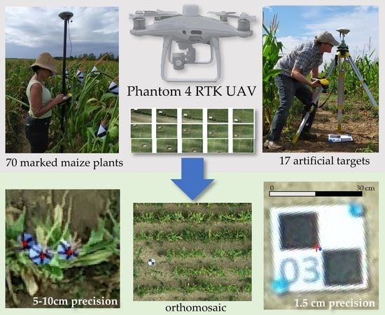
:To implement agricultural practices that are more respectful of the environment, precision agriculture methods for monitoring crop heterogeneity are becoming more and more spatially detailed. The objective of this study was to evaluate the potential of Ultra-High-Resolution UAV images with centimeter GNSS positioning for plant-scale monitoring. A Dji Phantom 4 RTK UAV with a 20 MPixel RGB camera was used, flying at an altitude of 25 m (0.7 cm resolution). This study was conducted on an experimental plot sown with maize. A centimeter-precision Trimble Geo7x GNSS receiver was used for the field measurements. After evaluating the precision of the UAV’s RTK antenna in static mode on the ground, the positions of 17 artificial targets and 70 maize plants were measured during a series of flights in different RTK modes. Agisoft Metashape software was used. The error in position of the UAV RTK antenna in static mode on the ground was less than one centimeter, in terms of both planimetry and elevation. The horizontal position error measured in flight on the 17 targets was less than 1.5 cm, while it was 2.9 cm in terms of elevation. Finally, according to the RTK modes, at least 81% of the corn plants were localized to within 5 cm of their position, and 95% to within 10 cm.
1. Introduction
Tomorrow’s challenges faced by agriculture are very important, and sometimes contradictory. Agriculture must adapt to climate change, even though it contributes to it, and must reduce its energy use and greenhouse gas emissions. According to the United Nations population division [1], the global population is expected to reach 9.7 billion by 2050; in order to meet demand, agriculture will then need to produce almost 50 percent more food than it did in 2012, according to the FAO [2]. To reconcile these two challenges faced by agriculture, i.e., to produce more food but in a sustainable way, precision agriculture (PA) provides technological tools for the optimized site-specific management of practices that are able to reduce the environmental footprint of agriculture. The OECD is encouraging work on PA in order to enhance sustainability and reduce risks associated with pesticides [3]. The transition to sustainable agriculture must be accelerated in order to reduce environmental pollution resulting from the intensive use of pesticides and fertilizers. In PA approaches, global navigation satellite systems (GNSS) and observation sensors are used to monitor the development of crops in a plot, both in space and time, delineating site-specific management zones [4] in which different settings for agricultural operations can be defined. Proximal sensors are mounted on ground-based platforms such as tractors, while remote sensing sensors are mounted on satellite, aerial and, more recently, UAV platforms [5]. Over the last decade, with the miniaturization of sensors, almost all types of sensors have been adapted to UAVs and used by the authors [6], including: (i) metric RGB cameras [7], (ii) non-metric RGB cameras [8], (iii) multispectral cameras [9], (iv) hyperspectral cameras [10,11], (v) LiDAR [12], (vi) thermal cameras [13], and (vii) GNSS reflectometry [14]. The biophysical variables of remotely sensed crops, i.e., leaf area index (LAI), normalized difference vegetation index (NDVI), fraction of photosynthetically active radiation (FPAR), chlorophyll content, and 3D crop surface model (CSM), are usually used to estimate aboveground biomass (AGB) on the basis of images obtained using a UAV [15]. The crop analysis scale in a plot has evolved a lot with the evolution of the spatiotemporal resolution of remote sensing sensors. At the beginning of satellite remote sensing with Landsat 1 in the 1970s, a spatial resolution of 80 m and a temporal resolution of 18 days allowed only simplified crop monitoring at the hectare scale; nowadays, with the Sentinel 2 satellite, for example, the spatial resolution is 10 m, or one hundredth of a hectare, and the temporal resolution is less than five days [5], enabling the use of PA in applications such as nitrogen fertilizer modulation. However, the availability of satellite images is sometimes compromised by cloud cover, and some uses are limited by the resolution of the satellites, such as early detection of weed, disease, or pest attacks; for these reasons, the use of UAVs in PA has been developing for the last decade; UAVs offer several advantages for vegetation monitoring, in that they can fly at very low altitudes, thus producing images with very high resolution, and flights can be scheduled with great flexibility in order to match the timing of growth stages imposed by the evolution of the crop over time [16]. For cameras with equivalent quality, the most detailed resolution can generally be obtained using rotary-wing UAVs, which can fly at a lower altitude than fixed-wing UAVs; rotary-wing UAVs also have better stability in flight, which contributes to better quality of the acquired images. Inertial measurement unit (IMU) and Global Navigation Satellite System (GNSS) receivers on board UAVs are used to determine the absolute position and orientation of the camera during flights, and Real-Time Kinematic (RTK) systems can also be used to improve GNSS accuracy to a few centimeters by using a correction signal from a fixed base station [17]. Several UAV models have now been equipped with RTK, and are starting to see use from several authors, such as the Sensefly eBee rtk [18,19,20,21] or the DJI phantom 4 RTK or matrix [22,23].
In this study, the main objective was to evaluate the potential of a UAV equipped with a centimetric GNSS to locate and track plants or small groups of plants in a crop over time. To do so, the accuracy of the UAV’s RTK centimetric GNSS receiver was first evaluated on the ground, then in flight on artificial targets evenly distributed in the study plot, and finally in flight, monitoring 70 maize plants with colored markers.
2. Materials and Methods
2.1. The Study Area
This study was conducted on the “QualiAgro” experimental plot [24], which was set up by the National Research Institute for Agriculture, food, and Environment (INRAE) and Veolia Environment Research and Innovation, in 1998. QualiAgro is part of the SOERE-PRO French research network on organic residues observatories. A long-term agronomic experiment is conducted on QualiAgro to study the effect of exogenous organic matter (EOM) applications on crop development. This 6 ha field is in the Paris region, France (48.8965° N, 1.975° E) (Figure 1a). Half of the field was sown in maize on 27 April 2020 with the MAS 220.V seed [25] from the Mas Seeds company [26]. UAV experimentation was carried out on a 0.5 ha sub-zone within the maize plot (Figure 1b). Maize was planted with an inter-row distance of 80 cm (Figure 1c), the average distance between plants in the same row was about 22.5 cm, with a minimum at 12 cm and a maximum at 47 cm.
2.2. The Unmanned Aerial Vehicule
A light quad-copter UAV was used for this study: the DJI Phantom 4 RTK (P4-RTK). It is a relatively recent UAV model from DJI, which came on the market at the end of 2018 (Figure 2a). P4-RTK is an easy-to-use and compact system that was designed for the acquisition of photogrammetric data with high geographic accuracy [27]. Its 20 Megapixel, 24 mm (35 mm equivalent) camera is mounted on a motorized gimbal (Figure 2d); with its mechanical shutter, the P4-RTK can move around while taking photos without the risk of blurring associated with the camera’s shutter (rolling shutter). The P4-RTK remote controller (Figure 2b) has a transmission range up to 7 km and the GS RTK application is preinstalled in the controller to plan flight paths and perform photogrammetry or waypoint flight operations. The maximum flight time with the P4-RTK battery was between 20 and 30 min, P4-RTK was equipped with six additional batteries to be able to carry out a series of flights in the same field day. P4-RTK GNSS receiver is multi-constellation and multi-frequency, it is compatible with the signals: GPS (L1/L2); GLONASS (L1/L2); BeiDou (B1/B2) and Galileo (E1/E2). It can operate in several modes: simple GNSS; RTK with the DJI D-RTK2 base station (Figure 2c); network RTK (NRTK) with an NRTK service provider; and post-processed kinematic (PPK) using raw satellite observations recorded during the flight. A Parrot Sequoia multispectral camera was also used (Figure 2e), it is fixed to the P4-RTK feet, using a special support and therefore does not have a motorized gimbal. Sequoia’s Sunshine sensor (Figure 2f) was fixed above the body of the P4-RTK on a small pole so as not to be disturbed by shadows.
2.3. Reference Measurement Method for GCP Positions
GCPs were used several times in the study as reference points on the ground to estimate the geographical precision of UAV’s data; it was therefore essential to determine GCPs geographical coordinates by a reference method with centimeter precision, and the Trimble Geo7x GNSS receiver was used for this (Figure 3a). Trimble Geo7x is a differential GNSS (DGNSS) designed as a rugged handheld which is a complete solution for performing high-precision surveys in the field. Geo7x is a dual-frequency receiver that has 220 channels and can work with GPS, GLONASS, BEIDOU, GALILEO and QZSS constellations; it has an integrated antenna and can also be connected to an external one (Figure 3). Geo7x can be used in three different ways in the field to make position surveys, in order of increasing precision: (i) hand-held using the integrated antenna (Figure 3b); (ii) with an external antenna mounted on a surveyor’s pole (Figure 3c); (iii) with an external antenna mounted on a tripod (Figure 3d).
The precision in the hand-held mode is not sufficient; in fact, it is not possible to place the phase center of the antenna precisely vertically to the measurement point; we estimate that there is an error of a few centimeters to a few tens of centimeters. The precision with the surveyor’s pole is better, since the height between the measuring point and the phase center is fixed, in this case at two meters. However, although the pole is equipped with a spirit level, it is not always easy to maintain exact verticality, and this error of angle generates an error in the estimated position on the ground of the measured point (Figure 4a). The offset D between the estimated position and the true position, depending on alpha (pole inclination) angle and H (pole height), is given by Equation (1).
For an angle of one degree, although being very small (Figure 4b), the difference D on the ground is 0.035 m; it is, therefore, difficult to guarantee measurements with centimeter precision in this mode. Only the use of a surveyor’s tripod makes it possible to position the phase center of the antenna vertically to the point to be measured. A Leica GDF322 professional tribrach with optical plummet was used with the tripod for greater accuracy of vertical alignment (Figure 4d); the centering accuracy was 0.5 mm at a height of 1.5 m. The positioning of the tripod with its optical plummet means that the measurement takes much longer than with the rod, requiring up to ten minutes per measurement.
The precision of the pole and tripod GNSS survey modes was tested on a geodesic point of the French geodesic network (RGF) at the Chavenay airport (Figure 5), the position of which was known with centimeter precision. The coordinates of the geodesic point were downloaded from the IGN geodesic files website [28].
Geo7x coordinates were finally projected in meters in the French Lambert 93 system (L93). Elevation data were measured in height above the ellipsoid (HAE). The mean error (ME) (Equation (2)) and the root mean square error (RMSE) (Equation (3)) were calculated between the Geo7x and the RGF coordinates (reference), for XL93, YL93 and ZL93.
where Vm is the measured value and Vref the reference one.
The Horizontal Error in the X/Y plane (HE) was evaluated as the Euclidean distance (Equation (4)).
2.4. Measurement of the P4-RTK DGNSS Receiver Accuracy in Static Mode on the Ground
To assess the best possible precision of the Phantom’s DGNSS antenna with its D-RTK2 base station, a first experiment was carried out with the UAV in static mode on the ground. Two GCPs were fixed to the ground (Figure 6a) and their position was determined to centimeter precision, with the Trimble Geo7x receiver on a tripod, as seen previously.
The D-RTK2 base station was stationed above the first GCP and programmed with the coordinates measured with the Trimble Geo7x. The second GCP was a white wooden board, with a cross drawn in its center with a black marker (Figure 6b), the camera pitch angle was set to −90° and the camera was centered on the black cross (Figure 6c). the board was placed horizontally with a spirit level. To perfectly center the drone’s camera on the cross, the “Custom Aim” application [12] was installed on the Android system of the remote controller. Custom Aim was used to create a red crosshair overlay at the center of the display, on top of the GS RTK application (Figure 6d). In GS RTK, in Fly mode, the camera video appears live on screen. The camera was centered by sliding the UAV on the board until the black cross was centered on the red crosshairs on the screen. The offset between the phase center of the P4-RTK antenna and the center of the camera’s CMOS was already applied in real time by the DJI algorithm to the coordinates saved in the image EXIF (Figure 7).
Eighty repetitions of the measurement were carried out; for this, the UAV was rotated around its vertical axis, according to the eight cardinal directions (Figure 8). For each position, 10 images were taken to record the geographic coordinates and the angles of the UAV as an image geotag.
The ExifTool software [29] was used as a command line in Windows 10 to extract all the image exif in the images directory as a csv file (Equation (5)).
The “−c%.8f” option was essential to force the output of the GNSS coordinates in latitude/longitude with eight digits after the decimal dot, because rounding was observed without this option, which resulted in the loss of centimeter precision. Coordinates were finally projected in meters in the French Lambert 93 system using CIRCE v 5.1 software [30] from the National Geographic Institute. The ME (Equation (2)), RMSE (Equation (3)) and HE error (Equation (4)) were calculated between the P4-RTK and the Geo7x coordinates, for XL93, YL93 and ZL93. As suggested by Štroner et al. [31] the global mean error between the P4-RTK measured and the reference positions was calculated for the detection of a systematic error. In case of no systematic error, global ME should be equal to zero.
2.5. Comparison of Different GNSS Modes in Flight
2.5.1. GCPs
A surveyor’s terminal (Figure 9a) was installed at the entrance to the study area to serve as a reference point for the DRTK-2 base station. The position was determined with the Trimble Geo7x receiver and was checked during four different tripod setups to validate it to the centimeter. Two garden slabs fitted with a cross and a surveyor’s nail (Figure 9b) were semi-buried at two points in the study area to serve as permanent GCPs. Fifteen cardboard targets (Figure 9c) were fixed to the ground with stakes to serve as temporary GCPs for one day of measurements.
The 15 targets were distributed more or less evenly throughout the measurement area (Figure 10). All GCP positions were recorded with the Geo7x terminal in tripod mode (Figure 9d). Seventy maize plants, spread over three rows, were marked to be located in the images of the various UAV flights. The markers were made with purple discs printed with black concentric lines towards its center (Figure 9e), which were cut and bent in the shape of a cone to be clearly visible from the air at different viewing angles, the concentric lines allow the stalk of the maize plant to be more precisely located in the images. The markers were attached with a clothes pin to the top leaf of the plant. The position of the 70 marked plants was recorded with the Geo7x receiver. Since it wasn’t possible to record the maize positions with the tripod, as the plants were too high, the positions were recorded with the pole at an accuracy of a few centimeters (Figure 11).
2.5.2. RTK Mode with the D-RTK2 Base Station Antenna
The optional Dji D-RTK2 base station was used. D-RTK2 Station is a high-precision GNSS receiver that supports all major global satellite navigation systems, providing real-time differential corrections to UAV to achieve centimeter-level positioning accuracy (Figure 12).
To improve the positioning of the D-RTK2 base, a spirit level larger than the one integrated in the tripod was fixed on the pole (Figure 13).
2.5.3. RTK Mode with the French Teria Network RTK Service
The network RTK service used the remote controller instead of the base station for differential data. The Teria network RTK (NRTK) service was created in 2005 at the request of the order of French expert surveyors. Teria is a multi-constellation service based on networked GNSS base stations. The network is made up of more than 200 stations. The stations are connected by a wired network to a server, which centralizes all the information. The exchanges between the server and the GNSS mobiles are performed by 4G wireless internet (Figure 14).
In this study, we used the SIM card and M2M (machine to machine) Teria subscription of the Trimble Geo7x DGNSS receiver, which was installed in the 4G key of the Phantom remote controller. In the Phantom configuration screen, RTK mode was activated, the type of service was set to “Custom network RTK”, and the access parameters of the server (IP address and login) were entered.
2.5.4. Simple GNSS Mode
For this flight, RTK mode was disabled on the drone’s remote controller so that it could operate only in simple GNSS mode.
2.5.5. PPK Mode Using RTKLIB and the French “RGP” Network
The P4-RTK stores the satellite observation data for Post-Process Kinematic (PPK). After a flight in simple GNSS mode, the RINEX (Receiver Independent Exchange Format) file of satellites observations, with “obs” extension, was in the image folder of the P4-RTK remote controller. The file was opened in a text editor to find out the precise first and last observation time of the flight (Figure 15).
The IXSG GNSS station of the city Saint-Germain-en-Laye, which was closest to QualiAgro plot (10 km), was used for the PPK corrections. The IXSG station is a part of the French permanent GNSS network (RGP) from the National Geographic Institute (IGN). Rinex file was downloaded from the RGP website [32] for GPS, Glonass and Galileo satellites with a time step of one second and for the time period corresponding to the P4-RTK Rinex file. It was important to choose the time output format in weeks and seconds, as this was the format of the P4-RTK “timestamp.MRK” file with which it was then combined. The P4-RTK and station Rinex files were processed with the rtkpost software of the rtklib project [33]. The main options used for rtkpost are summarized in Table 1.
The resulting file “100_0340_Rinex.pos” contained all the GNSS-corrected positions measured at regular time intervals during the flight, but not precisely those of the image shots; it was necessary to interpolate the image positions. The “100_0340_Timestamp.MRK” file recorded UAV information for each shot in the P4-RTK remote controller, especially the precise time of image acquisition. The image positions at RTK accuracy were interpolated from the positions in the 100_0340_Rinex.pos file based on time (Figure 16).
The precise camera center (CC) position was calculated from the GNSS antenna phase center (PC) position (Figure 17). During the flight, P4-RTK recorded the offset in mm between PC and CC in the Timestamp.MRK file considering the roll, pitch and yaw angles. Offsets in the north, east and vertical directions were in columns 4, 5 and 6 of the file, respectively. North offset was added to latitude and east offset to longitude, while vertical offset was subtracted from elevation.
The Aerotas P4RTK PPK Adjustments tool for Excel V1.0 was used for these previous calculations [34]. Finally, the positions were exported as a csv file and imported into Metashape as new camera references in place of the initial positions defined from the images EXIF.
2.6. The UAV Flights
Eight UAV flights were conducted over two days, 27 August 2020 and 7 September 2020; five of these flights were used for this study. The details of the flight parameters are presented in Table 2. Three flights (f1, f6 and f7) were designed with the same flight plan, at 25 m Above Ground Level (AGL), to evaluate the performance of different GNSS modes.
Flight f4 was a repetition of flight f1 with a different flying direction (Figure 18).
Flight f5 was like f4 but at 40 m AGL.
2.7. Photogrammetric Reconstruction
Due to the UAV’s low flight altitude, the photographic field of a single image covered only a small part of the area to be mapped. A mosaicking operation was performed to “merge” all the images into one (ortho-mosaic) that covered the entire study area. The method used for this was a 3D photogrammetric reconstruction with the Agisoft Metashape Professional v 1.7.4 software. The photogrammetry calculation was also used to correct the image distortions and to produce the results in a geographic coordinate system to be used in a GIS, thanks to the use of the GNSS positions in the images exif. As the UAV moved along the flight path between two successive positions O1 and O2 (Figure 19), the position P of a maize plant was projected in the two images at P1 and P2, respectively. P1 and P2 are homologous points, i.e., the same point of detail (key point) of the same maize plant in each of the two images. In Metashape, before any treatment, if the source data include RTK/PPK GNSS measurements, it is important to verify, and if necessary, change the accuracy values to 0.01 m for all the cameras; otherwise, the default accuracy value (10 m) will be assumed for all camera coordinates and the processing results will not be referenced with the expected accuracy. Usually, if the “load camera location accuracy from XMP” option is selected, Metashape automatically recovers the accuracy in the images exif. At the first alignment step of the processing workflow, Metashape found the camera position and orientation for each image and detected key points in the images and calculated their SIFT-like [35] descriptors. Descriptors are invariant to translation, rotation, and scaling transformations and robust to perspective and illumination variations; they were used to match identical key points between images; key points that were found in two or more images are also called tie points, and their positions were used to reconstruct the 3D scene structure.
The triangle o1 o2 P defines the so-called equipolar plane, and the distance between P1 and P2 is also called the disparity (d). The depth map, which provides the information on the distance of maize plants to the camera, was produced from the disparity map. Ullman’s Structure from Motion (SfM) theorem [36] showed that the 3D structure of rigid objects can be retrieved from their 2D projected positions in images; the result was a 3D sparse point cloud. According to the Metashape documentation, it is recommended to perform camera optimization by activating the “Fit additional corrections” option, which may be helpful for the datasets acquired with the DJI P4-RTK drone when no GCPs are used [37]. A densification step was then applied to obtain a detailed point cloud, called a dense cloud. MNS was built from the dense cloud, and finally an ortho-mosaic image was calculated. The main parameters used with Metashape are reported in Table 3. A Dell precision T7910 workstation was used, with an Intel dual Xeon 2.4 Ghz processor with 20 cores, 128 GB RAM and an NVIDIA Quadro M6000 24 GB graphic card.
The 3D reconstruction is all the better, as the number of images where the same key point is visible is important; this implies an important geographical overlap between neighboring images in the flight plan (Figure 20).
The overlap rate was set when the flight plan was created with the GS RTK application. An 80% rate was defined as the forward overlap, and a 70% rate was set between two parallel lines (side overlap). This is a very important setting for obtaining good-quality results, and a rate of 60% is the minimum; most often, the rate is set between 70% and 80%. Table 4 presents the 12 reconstructions that were computed with Agisoft Metashape. The first five reconstructions correspond to the five selected flights (f1, f4, f5, f6, f7). R_7_ppk reconstruction uses the same images as R_7, but with GNSS positions that were post-processed with RGP network data.
Three reconstructions were computed using GCPs as position markers to help the alignment step in Metashape, R_1_1gcp, R_1_3gcp and R_1_17gcp with one, three and seventeen GCPs, respectively (Figure 21). The GCPs were used in this case as control points at the alignment step in Metashape, and not only as check points. GCPs are often used in Metashape to improve the accuracy of the results. Each GCP was manually positioned very precisely in each image; this work was greatly facilitated by Metashape’s GCP guided positioning system, which once the GCP was placed on a first image, automatically calculated its position on all other images, before finally being refined manually.
Reconstruction R_1_4 was a combination of the f1 and f4 flights that had orthogonal flight directions (Figure 18), this is an often-recommended configuration for improving the quality of the final ortho-mosaic. Reconstruction R_1_5 was a combination of flights f1 and f5, which were at different flight heights, at 25 m and 40 m above ground level, respectively. Finally, reconstruction R_1_4_5 was the combination of flights f1, f4 and f5.
2.8. GCP Position Accuracy Evaluation
Each ortho-mosaic and MNS produced with Agisoft Metashape was then exported as Geotiff files and displayed in QGIS software. The center of each GCP was manually digitized from the image in a point layer (Figure 22). The X and Y coordinate values were added as new fields in the points layer table using the QGIS field calculator, and elevation values were extracted from the MNS layer at the points position using the QGIS raster analysis function “Sample raster values”. All these data were gathered in an excel sheet, and HE distances between the target centers and their reference position (GNSS) were calculated. Vertical error (VE) was also calculated.
2.9. Evaluation of the Accuracy of Maize Plant Position in Ortho-Mosaics
For each UAV flight, the ortho-mosaic was displayed in QGIS and the position of the maize markers was digitized in a point layer. The digitized point was on the intersection of the black lines printed on the marker which was the tip of the cone that was on the maize stem. These positions were compared to the GNNS surveys to calculate HE distance. Basic HE statistics were calculated for each reconstruction; the percentage of the maize plants’ population for which the horizontal error was within a distance interval was also calculated. The distances that were considered were: (i) between 0 and 5 cm; (ii) between 5 and 10 cm; (iii) between 0 and 10 cm; and (iv) greater than 10 cm.
3. Results
3.1. Reference Measurement Method for GCP Positions
The accuracies of the pole and tripod GNSS survey measured on the basis of Chavenay II geodesic points are presented in Table 5.
The horizontal accuracy obtained in tripod mode (Figure 23) is 1.1 cm, which is within the manufacturer’s specifications for the device. In pole mode, the horizontal precision falls to 4.3 cm, which corresponds well with the precision that can be expected from this mode of surveying, considering the difficulty in maintaining the pole perfectly vertically with respect to the measured point. The vertical accuracy is similar to the horizontal accuracy, and slightly lower than in tripod mode, where it is 1.6 cm.
3.2. P4-RTK DGNSS Receiver Accuracy in Static Mode on the Ground
The results of the accuracy of the P4-RTK DGNSS receiver in static ground mode with its D-RTK2 station correction are presented in Table 6. The average error for the 80 measurements was lower than one centimeter in terms of both planimetry (X,Y) and elevation (Z). The lowest horizontal error was 0.3 cm, while the highest was 1.2 cm.
3.3. Photogrammetric Reconstruction
Table 7 shows the main characteristics of the 12 reconstruction results obtained using Agisoft Metashape.
The ortho-mosaic computed by Metashape for the R-6 reconstruction (flight number 6) is shown in Figure 25. The images at different scales show the level of detail that can be obtained with sub-centimeter-resolution images.
3.4. GCP Position Accuracy According to the Different Reconstructions
Figure 26 shows the ortho-mosaic of the R_1 reconstruction, displayed in QGIS software, zoomed in on the 17 GCPs; the position of each target measured in the field with the Geo7x at centimeter accuracy is overlaid. All 17 targets appear to be visually very well centered on their reference positions as measured by the GNSS receiver.
Table 8 presents the statistics for the horizontal and vertical GCP positioning errors for all reconstructions. Table A1 shows the details of individual errors for each GCP in the cases of the R_1, R_5, R_6, R_7ppk and R_1_1gcp reconstructions.
A comparison of the mean values of HE obtained with the different GNSS modes is presented in Figure 27. The accuracies obtained with the D-RTK2 base station and with the NRTK TERIA mode were almost identical, i.e., 1.1 and 1.2 cm, respectively.
In simple GNSS mode without correction, the accuracy was 35 cm. After post-processing the GNSS surveys in ppk mode, the accuracy was 2.3 cm. Using GCPs as a control point during the alignment step in Metashape does not improve planimetric accuracy; the mean HE is identical to (i.e., within one millimeter of) that without GCP or with 1, 3 or 17. On the other hand, the use of GCP improves the accuracy in elevation, with the mean VE without GCP being 2.9 cm (R_1), while with 1 GCP it drops to 2.1 cm, and with 3 or 17 GCPs it reaches as low as 1.7 cm; 17 GCPs ultimately results in a precision no greater than with 3. Reconstructions that combine a flight at a height of 25 m with flight 5 at 40 m, without GCP (R_1_5 and R_1_4_5) result in a 30% improvement in elevation accuracy, which is comparable to when using one GCP for flight 1 (R1_1gcp). For the R_7 reconstruction in simple GNSS mode without correction, the mean VE is about one meter in elevation. For all flights at a height of 25 m that used differential correction of the GNSS signal, without GCP (R_1, R_4, R_6), the planimetric accuracy seems stable between flights, at between 1.1 and 1.2 cm. For the R_5 reconstruction, which employed the same conditions but at a 40 m flight height, the average HE was 1.6 cm, which is comparable; indeed, when considering GSD (0.7 cm vs. 1.1 cm for R_5), for all those flights, the mean HE corresponds to about 1.6 times the GSD. For these same flights, the altimetric accuracy seems to be less stable, varying between 2.3 and 3.2 cm and even reaching 6.7 cm for flight 5 at an altitude of 40 m. VE appears to be more stable when using GCPs or a combination of two flight altitudes. The combination of two flights at the same altitude (R_1_4) does not seem to improve either horizontal or vertical accuracy. The use of two flights at a height of 25 m in combination with the flight at 40 m (R1_4_5) provides no improvement compared to R_1_5.
3.5. Maize Plant Position Accuracy according to the Different Reconstructions
Figure 28 shows, among the three monitored rows, the central maize row on the R_1 ortho-mosaic; at this resolution of 0.7 cm, the purple markers are easily visible, as well as their concentric black lines, the intersections of which indicate the plant stem. The GNSS positions measured with the Trimble Geo7x are displayed on top of the image to appreciate their distance to the markers.
Statistics based on HE between the marker positions and the GNSS position measured on the ground are presented in Table 9. For the D-RTK2 mode, the mean HE ranges from 1.9 cm to 3.2 cm, for the Teria mode the mean HE is 4.0 cm, and for the PPK mode it is 5.4 cm. For all reconstructions, the maximum HE is quite high, between 14.8 cm and 39.1 cm, but the very low number of plants for which HE is higher than ten centimeters shows that it is only for a few isolated plants.
Figure 29a represents, for each reconstruction, the percentage of the 70 maize plants that were located on the ortho-image within five centimeters of their GNSS position surveyed in the field with the Geo7x. For all reconstructions based on D-RTK2 acquisitions, this percentage is between 81% and 90%. R_6 Teria mode and R7_ppk reconstructions are slightly less accurate, at 69% and 60%, respectively. As for the R_7 reconstruction in simple GNSS mode, its accuracy is insufficient for locating the plants to within five centimeters.
4. Discussion
4.1. GNSS Reference Measurement with Trimble Geo7x
To ensure that the positions of the targets used as ground check points were determined with centimetric accuracy, we first analyzed the survey performed using the Trimble Geo7x “centimetric” GNSS receiver from a metrology point of view. Measurements on a geodesic point showed that the precision that could be achieved when using a surveyor’s pole with a bubble level was on the order of only four centimeters, whereas performing measurements with a tripod equipped with an optical plummet made it possible to achieve centimeter precision. It is common for DGNSS receiver users to think that because the manufacturer’s specifications give a centimeter accuracy, that the accuracy of the measurement will automatically be at that same accuracy; this is only true if it can be guaranteed that the phase center of the antenna is perfectly vertical to the point being measured, which can usually only be achieved by setting up a tripod on the point. Authors often do not describe in sufficient detail the process used for GCP GNSS measurements, which makes it impossible to estimate its real precision; Štroner et al. [38], in their study on the georeferencing of RTK drone images, describe in detail the GNSS measurement of GCPs on the basis of three repetitions, before, between, and after a series of flights, and report a realistic accuracy of three centimeters. The disadvantage of the tripod method compared to the pole method is that it takes much longer, requiring about ten minutes per measurement. A new range of GNSS antennas has recently appeared on the market that could help in achieving rapid pole surveys that are as accurate as with a tripod, such as the Leica iCON gps 70 [39], which measures a point without the need to keep the pole vertical and level the bubble. An inertial measurement unit is integrated into the iCON’s antenna, offering permanent real-time tilt compensation. This type of device has interesting potential when performing studies, such as the one presented in this article, that require a large number of very precisely located GCPs.
4.2. P4-RTK DGNSS Receiver Accuracy
The GNSS antenna of the P4-RTK connected to its D-RTK2 station was evaluated in this study in static mode on the ground as having an accuracy of less than one centimeter in terms of planimetry and elevation, which is in accordance with the specifications of the DJI manufacturer. Measurements performed by orienting the UAV along the eight cardinal directions while being centered on the GCP did not indicate any directional effect on the planimetry and elevation accuracies; this seems to show that the P4-RTK was able to achieve good correction of the offset between the phase center of the antenna and the optical center of the camera according to the different attitudes of the UAV (lever arm correction). To refine this observation, it would be necessary to carry out measurements with UAV tilt effects, to check whether the calculation integrates the position taken by the motorized gimbal well for lever arm correction in any attitude. The graph of these measurements (Figure 24) shows a small systematic error, which may arise from the difficulty of very precisely setting the D-RTK2 station up due to the poor quality of its tripod. Indeed, this tripod is too light, the fixation system of the pole can cause a slight displacement, and the bubble levels are not very precise. For the continuation of this study, a “GPS” thread adaptor was ordered in order to be able to mount the D-RTK2 antenna on a good-quality tripod with an optical plummet.
The accuracy of the positions measured for artificial targets in a series of flights at 25 m AGL in DGNSS mode (D-RTK2 or NRTK-Teria) was about one centimeter in terms of planimetry, which corresponds to about one and a half times the GSD (from 1.5 to 1.7 GSD, depending on the RTK mode). This result remained the same regardless of whether or not GCPs were used as control points in the photogrammetric alignment step with the Metashape software. In ppk mode, the accuracy was 2.3 cm, which is worse than the accuracies in the D-RTK2 and Teria modes; this can be explained by the distance to the RGP station that was used (10 km); indeed, it can generally be considered that the additional error due to this distance corresponds to one part per million (ppm), i.e., one centimeter for every ten kilometers; the best accuracy that can be expected in ppk mode with this station is therefore two centimeters. As Cledat et al. pointed out in their study on the use of RTK UAVs in complex natural environments [19], the ppk mode may be preferable in the case of flights where there is a risk of loss of the real-time RTK correction signal or even of the GNSS signal. The precision of 1.5 GSD in terms of planimetry with an RTK UAV without GCPs is consistent with the results reported by other authors. Štroner et al. [31] obtained a level of accuracy of 1–2 GSD with a P4-RTK. Taddia et al. [40] carried out a series of flights with a P4-RTK at 80 m AGL (2 cm GSD), and also obtained an accuracy of 1.5 GSD in terms of planimetry without using GCP in RTK mode. Forlani et al. [41] obtained similar results with a Sensefly eBee-RTK fixed-wing UAV, flying at 90 m AGL with a GSD of 2.3 cm, in RTK or NRTK mode without using GCPs, and obtained a horizontal accuracy of about 1.2 GSD. The elevation accuracy obtained in this study with the P4-RTK on the ground was comparable to the horizontal accuracy, and was less than one centimeter (Table 6). During flight and on artificial targets, for the different DGNSS modes without GCP, elevation accuracy was more variable than planimetric accuracy (Table 8), with precision varying between 2.3 and 9.7 cm. The worst value was obtained in ppk mode, which can be explained, as for planimetric accuracy, by the distance from the RGP station that was used. The use of GCPs during the Metashape reconstructions led to an improvement in vertical precision. Reconstruction using a single GCP (R_1_1gcp) resulted in a VE of two centimeters, compared with the values obtained without GCP (R_1, R_4 and R_6), which varied between 2.3 and 3.2 cm. The use of three GCPs (R_1_3gcp) further improved the precision, with a VE value of 1.7 cm. On the other hand, the use of greater numbers of GCPs (17 for R_1_17gcp) did not seem to improve the vertical precision compared to when using three GCPs. Several authors have highlighted this type of systematic elevation error using UAVs equipped with GNNS RTK receivers without the use of GCPs [38,42,43], for the most part with rotary-wing UAVs, but also with fixed-wing UAVs as in the study carried out on direct georeferencing by Rabah et al. [20], where they used a Sensefly eBee RTK. This elevation error, which has sometimes been described as being “almost random” by some authors, could be due to the incorrect determination of the internal orientation parameters of the camera (i.e., focal length) by the photogrammetry software [38]. The results obtained in this study with respect to correcting this additional error in elevation using GCPs is consistent with the results obtained by other authors; for example, Forlani et al. [41] obtained vertical accuracies of 4.6 cm in RTK mode without GCPs, 3.2 cm with one GCP, and 2.3 cm with 12 GCPs, with a GSD of about 2.3 cm. Because the use of GCPs is time consuming in the field, other correction strategies have been explored by authors, such as combining flights at different altitudes; combining shots with different camera angles; combining flights with different orientations, for example, orthogonal to each other; and pre-calibration of the camera. In this study, the combination of two orientations in the R_1_4 reconstruction (Table 8) did not result in any improvement in elevation error, and the best correction was obtained for the R_1_5 reconstruction, which combined two flight altitudes (25 m and 40 m); Štroner et al. [38] came to the same conclusion. In the rest of this study, it is planned to analyze in more detail the effects of these different acquisition parameters on stabilizing the accuracy of elevation estimations. This may be important for crop biomass monitoring, since new approaches have been developed based on UAV Crop surface models to predict crop height [42,43].
4.3. Maize Plant Position Accuracy
The present study aimed to prove the possibility of using ultra-high-resolution UAV images coupled with centimetric GNSS localization to monitor a crop at the scale of individual plants or small groups of plants by more specifically analyzing the accuracy of plant positioning in the resulting ortho-mosaics. Position measurements in RTK or NRTK mode on four different flights (f1, f4, f5 and f6), which were carried out on 70 maize plants with markers that were visible in the ortho-images, showed that the individual location of each plant in the image could be found with an accuracy of less than ten centimeters in 95% of cases, and with an accuracy of less than five centimeters in 81% of cases. Deviations greater than 10 cm were observed on few plants; after visual analysis of these plants in the ortho-mosaics generated for several flights, it was noted that this corresponded to the movement of these plants between flights, which can probably be explained by a gust of wind, with some plants being more exposed than others. At the time of the drone acquisitions, at the end of August 2020, the height of the corn plants was about 1.5 m, giving them significant wind resistance. This imprecision, which may exist at certain stages of crop development, is, however, quite limited, since it is strongly advised that UAV flights be carried out in moderate winds. Having determined the positions of plants during a first flight, it must be possible to find those same plants in subsequent flights at different stages of development of the maize crop with an inter-row distance of 80 cm and an average distance between plants of the same row of 22.5 cm (Figure 1c). This can be particularly useful for following the development of diseases or damage caused by pests over time, starting from the sources of their appearance. Localization to individual plants is obviously easier with a crop such as maize, where the row spacing is often around 80 cm, than for wheat crops, where the row spacing is around 25 cm, and the plant density is therefore much greater. Monitoring in the latter case will tend to be on the scale of small groups of plants, rather than that of individual plants. Jin et al. [44] showed in a study on the counting of wheat plants by UAV with flights at very low altitudes (less than 7 m) the importance of having sufficiently fine image resolution to properly detect and locate individual plants, with the RMSE of the number of plants per m2 they obtained being directly related to the resolution of the images used. The remote controller supplied with the P4-RTK and its software (GS RTK) does not allow flights to be carried out at altitudes lower than 25 m, which limits the resolution that can be achieved (7 mm). Following this study, monitoring was started on agronomic trials in wheat; in order to achieve more detailed resolutions, a Dji GS SDK remote controller was acquired, with its GS PRO software, which allows flights to be performed at altitudes as low as 5 m, which corresponds to a resolution of about 1.4 mm.
5. Conclusions
We evaluated the performance of the P4-RTK GNSS receiver on artificial targets with very precisely known positions, and our results showed, an accuracy of less than one centimeter in static mode on the ground and an accuracy of about 1.5 GSD (lower than 1.5 cm in RTK mode) in flight. We tracked 70 maize plants, which were tagged, during a series of UAV flights and showed that for 81% of the plants, their position in the images between different flights could be retrieved with an accuracy of less than 5 cm (95% less than 10 cm). Considering a maize inter-row distance of 80 cm and an average distance between plants in the same row of 22.5 cm, the P4-RTK is potentially able to locate and thus monitor each plant individually over time using several UAV flights. Automatic maize plant detection from UAV images could then be used, as proposed by Velumani et al. [45] using deep learning methods, or Zhang et al. [46] who extracted each plant as an object and were able to estimate the distance between plants with an accuracy of about 10%. In France, the Azur drone company has obtained a derogation to the regulations on UAVs for its Skeyetech UAV [47] from the French Civil Aviation Authority (DGAC), allowing their operation in fully autonomous mode without any operator; a base placed outside serves as a shelter (designed to resist most extreme climatic conditions) in which the UAV is able to recharge automatically, while a removable roof releases the drone at the time of its mission, and a weather station is used to check the conditions before the flight. This is a surveillance UAV for sensitive industrial plants, but one can imagine that, in the relatively near future, such a system could be installed in farmyards with RTK UAVs, acting as a fully automated system that is able to go autonomously over a plot, and follow, plant by plant, the development of crop biomass or the appearance and development of disease outbreaks or pest attacks. In such a scenario, an evolution of aviation legislation would be necessary, but this is already in progress, with the European Union having defined U-space, which is the European unmanned traffic management system, as constituting four successive phases, the last of which (U4), planned for 2030, will authorize implementation of all U-space services, including high levels of automation [48].
Author Contributions
J.-M.G. designed the UAV experiments. Experiments were performed by J.-M.G. and D.H., J.-M.G. drafted the manuscript with help and contributions from all other authors. Analyses, figures, and tables were mainly performed and produced by J.-M.G. All authors have read and agreed to the published version of the manuscript.
Funding
This research was funded by AgroParisTech Paris-Saclay University Call for scientific projects, grant reference ToUHR-DRONAé (Ultra-High-Resolution Remote Sensing by UAV for the adaptation to Agroecological practices) and by the French national observatory networks “SOERE PRO” part of the AnaEE-France project of the French Investments for the Future (Investissements d’Avenir) program, implemented by the French National Research Agency (ANR) (ANR-11-INBS-0001). The field experiment QualiAgro has been managed since 1998 within a cooperation between INRAE and Veolia Research and Innovation.
Acknowledgments
The authors are grateful to Camille Resseguier, in charge of the daily management of the QualiAgro field experiment, for her very efficient organization of the experiments taking place on the plot and to Sabine Houot, who ensured the scientific coordination of the SOERE-PRO network and who allowed us to conduct this study on the QualiAgro plot.
Conflicts of Interest
The authors declare that they have no conflict of interest.
Appendix A

Table A1.
Horizontal (HE) and vertical error (VE) on the 17 GCP positions in meters, of the R_1, R_5, R_6, R_7ppk and R_1_1gcp reconstructions.
Table A1.
Horizontal (HE) and vertical error (VE) on the 17 GCP positions in meters, of the R_1, R_5, R_6, R_7ppk and R_1_1gcp reconstructions.
| GCP | R_1 HE m | R_1 VE m | R_5 HE m | R_5 VE m | R_6 HE m | R_6 VE m | R_7ppk HE m | R_7ppk VE m | R_1_1gcp HE m | R_1_1gcp VE m |
| F01 | 0.011 | 0.043 | 0.009 | 0.059 | 0.011 | 0.045 | 0.015 | 0.071 | 0.011 | 0.008 |
| F02 | 0.015 | 0.039 | 0.017 | 0.046 | 0.010 | 0.042 | 0.028 | 0.086 | 0.015 | 0.003 |
| G02 | 0.005 | 0.032 | 0.016 | 0.070 | 0.001 | 0.036 | 0.017 | 0.086 | 0.005 | 0.006 |
| G03 | 0.019 | 0.064 | 0.024 | 0.027 | 0.012 | 0.064 | 0.027 | 0.050 | 0.019 | 0.031 |
| G04 | 0.013 | 0.028 | 0.023 | 0.063 | 0.011 | 0.031 | 0.017 | 0.088 | 0.015 | 0.011 |
| G05 | 0.017 | 0.024 | 0.022 | 0.064 | 0.015 | 0.021 | 0.021 | 0.088 | 0.017 | 0.013 |
| G06 | 0.003 | 0.060 | 0.004 | 0.026 | 0.006 | 0.063 | 0.017 | 0.055 | 0.003 | 0.025 |
| G07 | 0.005 | 0.035 | 0.013 | 0.051 | 0.010 | 0.043 | 0.020 | 0.093 | 0.006 | 0.003 |
| G08 | 0.011 | 0.008 | 0.015 | 0.104 | 0.022 | 0.004 | 0.008 | 0.139 | 0.011 | 0.047 |
| G09 | 0.006 | 0.000 | 0.008 | 0.095 | 0.009 | 0.006 | 0.023 | 0.132 | 0.003 | 0.035 |
| G10 | 0.008 | 0.021 | 0.020 | 0.079 | 0.007 | 0.028 | 0.025 | 0.113 | 0.008 | 0.019 |
| G11 | 0.015 | 0.006 | 0.028 | 0.105 | 0.010 | 0.017 | 0.032 | 0.128 | 0.015 | 0.030 |
| G12 | 0.011 | 0.018 | 0.010 | 0.121 | 0.011 | 0.013 | 0.023 | 0.148 | 0.011 | 0.056 |
| G13 | 0.014 | 0.006 | 0.011 | 0.087 | 0.008 | 0.006 | 0.029 | 0.119 | 0.014 | 0.030 |
| G14 | 0.020 | 0.034 | 0.024 | 0.064 | 0.009 | 0.037 | 0.032 | 0.086 | 0.020 | 0.002 |
| G15 | 0.021 | 0.032 | 0.016 | 0.058 | 0.016 | 0.035 | 0.035 | 0.092 | 0.021 | 0.004 |
| G16 | 0.018 | 0.047 | 0.023 | 0.032 | 0.017 | 0.052 | 0.018 | 0.072 | 0.018 | 0.012 |
References
- World Population Prospects—Population Division—United Nations. Available online: https://population.un.org/wpp/ (accessed on 20 September 2021).
- The Future of Food and Agriculture: Trends and Challenges; Food and Agriculture Organization of the United Nations: Rome, Italy, 2017; ISBN 978-92-5-109551-5.
- OECD. Pesticides and Sustainable Pest Management Vision for the Future: A Cooperative Global Approach to the Regulation of Agricultural Pesticides and Sustainable Pest Management. Available online: https://www.oecd.org/chemicalsafety/pesticides-biocides/OECD-Pest-Vision-Final.pdf (accessed on 20 September 2021).
- Méndez-Vázquez, L.J.; Lira-Noriega, A.; Lasa-Covarrubias, R.; Cerdeira-Estrada, S. Delineation of Site-Specific Management Zones for Pest Control Purposes: Exploring Precision Agriculture and Species Distribution Modeling Approaches. Comput. Electron. Agric. 2019, 167, 105101. [Google Scholar] [CrossRef]
- Sishodia, R.P.; Ray, R.L.; Singh, S.K. Applications of Remote Sensing in Precision Agriculture: A Review. Remote Sens. 2020, 12, 3136. [Google Scholar] [CrossRef]
- Mulla, D.J. Twenty Five Years of Remote Sensing in Precision Agriculture: Key Advances and Remaining Knowledge Gaps. Biosyst. Eng. 2013, 114, 358–371. [Google Scholar] [CrossRef]
- IGN Caméra Légère IGN | IGN Lightweight Camera. Available online: http://www.ign.fr/institut/innovation/camera-legere-ign (accessed on 8 October 2020).
- Poblete-Echeverría, C.; Olmedo, G.F.; Ingram, B.; Bardeen, M. Detection and Segmentation of Vine Canopy in Ultra-High Spatial Resolution RGB Imagery Obtained from Unmanned Aerial Vehicle (UAV): A Case Study in a Commercial Vineyard. Remote Sens. 2017, 9, 268. [Google Scholar] [CrossRef] [Green Version]
- Deng, L.; Mao, Z.; Li, X.; Hu, Z.; Duan, F.; Yan, Y. UAV-Based Multispectral Remote Sensing for Precision Agriculture: A Comparison between Different Cameras. ISPRS J. Photogramm. Remote Sens. 2018, 146, 124–136. [Google Scholar] [CrossRef]
- Singh, P.; Pandey, P.C.; Petropoulos, G.P.; Pavlides, A.; Srivastava, P.K.; Koutsias, N.; Deng, K.A.K.; Bao, Y. 8—Hyperspectral Remote Sensing in Precision Agriculture: Present Status, Challenges, and Future Trends. In Hyperspectral Remote Sensing; Pandey, P.C., Srivastava, P.K., Balzter, H., Bhattacharya, B., Petropoulos, G.P., Eds.; Earth Observation; Elsevier: Amsterdam, The Netherlands, 2020; pp. 121–146. ISBN 978-0-08-102894-0. [Google Scholar]
- Zhang, Y.; Xia, C.; Zhang, X.; Cheng, X.; Feng, G.; Wang, Y.; Gao, Q. Estimating the Maize Biomass by Crop Height and Narrowband Vegetation Indices Derived from UAV-Based Hyperspectral Images. Ecol. Indic. 2021, 129, 107985. [Google Scholar] [CrossRef]
- Lin, Y.-C.; Habib, A. Quality Control and Crop Characterization Framework for Multi-Temporal UAV LiDAR Data over Mechanized Agricultural Fields. Remote Sens. Environ. 2021, 256, 112299. [Google Scholar] [CrossRef]
- Ortega-Farias, S.; Esteban-Condori, W.; Riveros-Burgos, C.; Fuentes-Peñailillo, F.; Bardeen, M. Evaluation of a Two-Source Patch Model to Estimate Vineyard Energy Balance Using High-Resolution Thermal Images Acquired by an Unmanned Aerial Vehicle (UAV). Agric. For. Meteorol. 2021, 304–305, 108433. [Google Scholar] [CrossRef]
- Van de Vyvere, L.; Desenfans, O. MISTRALE: Soil Moisture Mapping Service Based on a UAV-Embedded GNSS-Reflectometry Sensor. In Proceedings of the EGU General Assembly Conference Abstracts, Vienna, Austria, 17–22 April 2016; Volume 18, p. 5905. [Google Scholar]
- Xie, C.; Yang, C. A Review on Plant High-Throughput Phenotyping Traits Using UAV-Based Sensors. Comput. Electron. Agric. 2020, 178, 105731. [Google Scholar] [CrossRef]
- de Castro, A.I.; Shi, Y.; Maja, J.M.; Peña, J.M. UAVs for Vegetation Monitoring: Overview and Recent Scientific Contributions. Remote Sens. 2021, 13, 2139. [Google Scholar] [CrossRef]
- Ekaso, D.; Nex, F.; Kerle, N. Accuracy Assessment of Real-Time Kinematics (RTK) Measurements on Unmanned Aerial Vehicles (UAV) for Direct Geo-Referencing. Geo-Spat. Inf. Sci. 2020, 23, 165–181. [Google Scholar] [CrossRef] [Green Version]
- Benassi, F.; Dall’Asta, E.; Diotri, F.; Forlani, G.; Morra di Cella, U.; Roncella, R.; Santise, M. Testing Accuracy and Repeatability of UAV Blocks Oriented with GNSS-Supported Aerial Triangulation. Remote Sens. 2017, 9, 172. [Google Scholar] [CrossRef] [Green Version]
- Cledat, E.; Jospin, L.V.; Cucci, D.A.; Skaloud, J. Mapping Quality Prediction for RTK/PPK-Equipped Micro-Drones Operating in Complex Natural Environment. ISPRS J. Photogramm. Remote Sens. 2020, 167, 24–38. [Google Scholar] [CrossRef]
- Rabah, M.; Basiouny, M.; Ghanem, E.; Elhadary, A. Using RTK and VRS in Direct Geo-Referencing of the UAV Imagery. NRIAG J. Astron. Geophys. 2018, 7, 220–226. [Google Scholar] [CrossRef] [Green Version]
- González-García, J.; Swenson, R.L.; Gómez-Espinosa, A. Real-Time Kinematics Applied at Unmanned Aerial Vehicles Positioning for Orthophotography in Precision Agriculture. Comput. Electron. Agric. 2020, 177, 105695. [Google Scholar] [CrossRef]
- Yu, R.; Luo, Y.; Zhou, Q.; Zhang, X.; Wu, D.; Ren, L. Early Detection of Pine Wilt Disease Using Deep Learning Algorithms and UAV-Based Multispectral Imagery. For. Ecol. Manag. 2021, 497, 119493. [Google Scholar] [CrossRef]
- Xu, W.; Chen, P.; Zhan, Y.; Chen, S.; Zhang, L.; Lan, Y. Cotton Yield Estimation Model Based on Machine Learning Using Time Series UAV Remote Sensing Data. Int. J. Appl. Earth Obs. Geoinf. 2021, 104, 102511. [Google Scholar] [CrossRef]
- Inrae QualiAgro. Available online: http://www6.inra.fr/qualiagro_eng (accessed on 8 October 2020).
- Mas Seeds Maize Seed MAS 220.V. Available online: https://www.masseeds.fr/nos-cultures-et-semences/nos-semences/mais/mas-220v (accessed on 10 February 2022).
- Mas Seeds. Available online: https://www.masseeds.fr/ (accessed on 11 February 2022).
- DJI PHANTOM 4 RTK User Manual v2.4. Available online: https://dl.djicdn.com/downloads/phantom_4_rtk/20210716/Phantom_4_RTK_User_Manual_v2.4_EN.pdf (accessed on 3 September 2021).
- IGN Serveur de Fiches | Géodésie. Available online: https://geodesie.ign.fr/fiches (accessed on 6 September 2021).
- Harvey, P. ExifTool. Available online: https://exiftool.org/ (accessed on 4 September 2021).
- IGN Logiciels Circé | Géodésie. Available online: https://geodesie.ign.fr/index.php?page=circe (accessed on 4 September 2021).
- Štroner, M.; Urban, R.; Reindl, T.; Seidl, J.; Brouček, J. Evaluation of the Georeferencing Accuracy of a Photogrammetric Model Using a Quadrocopter with Onboard GNSS RTK. Sensors 2020, 20, 2318. [Google Scholar] [CrossRef] [Green Version]
- IGN RGP Network Map. Available online: http://rgp.ign.fr/ (accessed on 17 September 2021).
- rtklib RTKLIB: An Open Source Program Package for GNSS Positioning. Available online: http://www.rtklib.com/ (accessed on 17 September 2021).
- Aerotas Phantom 4 RTK—PPK Processing Workflow | Drone Data Processing. Available online: https://www.aerotas.com/phantom-4-rtk-ppk-processing-workflow (accessed on 17 September 2021).
- Lowe, D.G. Distinctive Image Features from Scale-Invariant Keypoints. Int. J. Comput. Vis. 2004, 60, 91–110. [Google Scholar] [CrossRef]
- Ullman, S. The Interpretation of Structure from Motion. Proc. R. Soc. Lond. B 1979, 203, 405–426. [Google Scholar] [CrossRef]
- Agisoft Agisoft Metashape User Manual—Professional Edition, Version 1.7 2021. Available online: https://www.agisoft.com/pdf/metashape-pro_1_7_en.pdf (accessed on 22 March 2022).
- Štroner, M.; Urban, R.; Seidl, J.; Reindl, T.; Brouček, J. Photogrammetry Using UAV-Mounted GNSS RTK: Georeferencing Strategies without GCPs. Remote Sens. 2021, 13, 1336. [Google Scholar] [CrossRef]
- Leica Geosystems Leica iCON GPS 70. Available online: https://leica-geosystems.com/fr-CH/products/construction-tps-and-gnss/smart-antennas/leica-icon-gps-70-series (accessed on 22 October 2021).
- Taddia, Y.; Stecchi, F.; Pellegrinelli, A. Using DJI Phantom 4 RTK Drone for Topographic Mapping of Coastal Areas. In Proceedings of the International Archives of the Photogrammetry, Remote Sensing and Spatial Information Sciences, Enschede, The Netherlands, 10–14 June 2019; Volume XLII-2/W13, pp. 625–630. [Google Scholar]
- Forlani, G.; Dall’Asta, E.; Diotri, F.; di Cella, U.M.; Roncella, R.; Santise, M. Quality Assessment of DSMs Produced from UAV Flights Georeferenced with On-Board RTK Positioning. Remote Sens. 2018, 10, 311. [Google Scholar] [CrossRef] [Green Version]
- Bendig, J.; Bolten, A.; Bennertz, S.; Broscheit, J.; Eichfuss, S.; Bareth, G. Estimating Biomass of Barley Using Crop Surface Models (CSMs) Derived from UAV-Based RGB Imaging. Remote Sens. 2014, 6, 10395–10412. [Google Scholar] [CrossRef] [Green Version]
- Gilliot, J.M.; Michelin, J.; Hadjard, D.; Houot, S. An Accurate Method for Predicting Spatial Variability of Maize Yield from UAV-Based Plant Height Estimation: A Tool for Monitoring Agronomic Field Experiments. Precis. Agric. 2020, 22, 897–921. [Google Scholar] [CrossRef]
- Jin, X.; Liu, S.; Baret, F.; Hemerlé, M.; Comar, A. Estimates of Plant Density of Wheat Crops at Emergence from Very Low Altitude UAV Imagery. Remote Sens. Environ. 2017, 198, 105–114. [Google Scholar] [CrossRef] [Green Version]
- Velumani, K.; Lopez-Lozano, R.; Madec, S.; Guo, W.; Gillet, J.; Comar, A.; Baret, F. Estimates of Maize Plant Density from UAV RGB Images Using Faster-RCNN Detection Model: Impact of the Spatial Resolution. Plant Phenomics 2021, 2021, 9824843. [Google Scholar] [CrossRef] [PubMed]
- Zhang, J.; Basso, B.; Price, R.F.; Putman, G.; Shuai, G. Estimating Plant Distance in Maize Using Unmanned Aerial Vehicle (UAV). PLoS ONE 2018, 13, e0195223. [Google Scholar] [CrossRef] [PubMed] [Green Version]
- Azur Drones Skeyetech—Autonomous Drone for Security and Safety. Available online: https://www.azurdrones.com/product/skeyetech/ (accessed on 22 March 2022).
- SESAR Join Undertaking U-Space Blueprint. Available online: https://www.sesarju.eu/sites/default/files/documents/reports/U-space%20Blueprint%20brochure%20final.PDF (accessed on 22 March 2022).
Figure 1.
Study area: (a) QualiAgro plot location in France; (b) study area in the QualiAgro plot; (c) planting of maize plants along two successive rows, in red the distance in centimeters, between two successive plants in a row (from a UAV ortho-image of 27 August 2020).
Figure 1.
Study area: (a) QualiAgro plot location in France; (b) study area in the QualiAgro plot; (c) planting of maize plants along two successive rows, in red the distance in centimeters, between two successive plants in a row (from a UAV ortho-image of 27 August 2020).
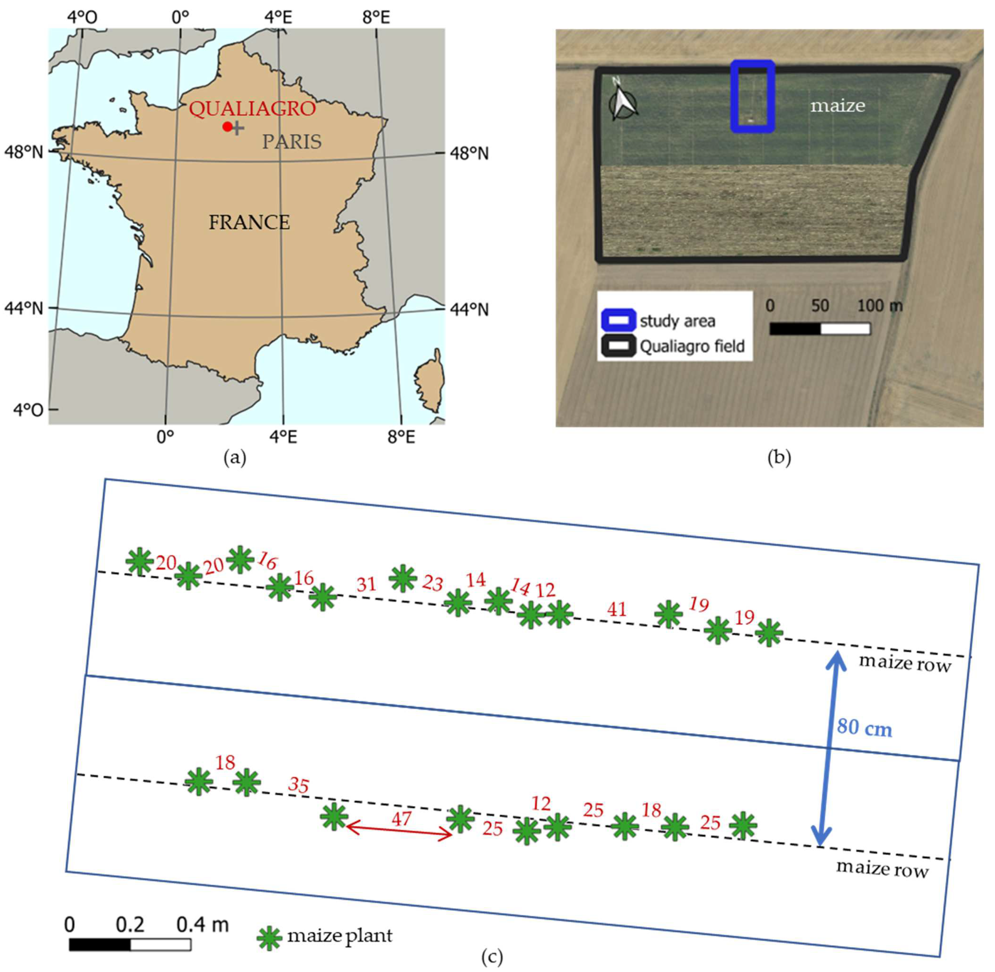
Figure 2.
Dji Phantom 4 RTK: (a) UAV; (b) remote controller; (c) D-RTK2 base station; (d) RGB camera on the motorized gimbal; (e) SEQUOIA multispectral camera; (f) light sensor; (g) GNSS antenna.
Figure 2.
Dji Phantom 4 RTK: (a) UAV; (b) remote controller; (c) D-RTK2 base station; (d) RGB camera on the motorized gimbal; (e) SEQUOIA multispectral camera; (f) light sensor; (g) GNSS antenna.

Figure 3.
Trimble Geo7x GNSS receiver: (a) Geo7x with integrated antenna; (b) hand-held mode; (c) external antenna on a pole; (d) external antenna on a tripod.
Figure 3.
Trimble Geo7x GNSS receiver: (a) Geo7x with integrated antenna; (b) hand-held mode; (c) external antenna on a pole; (d) external antenna on a tripod.
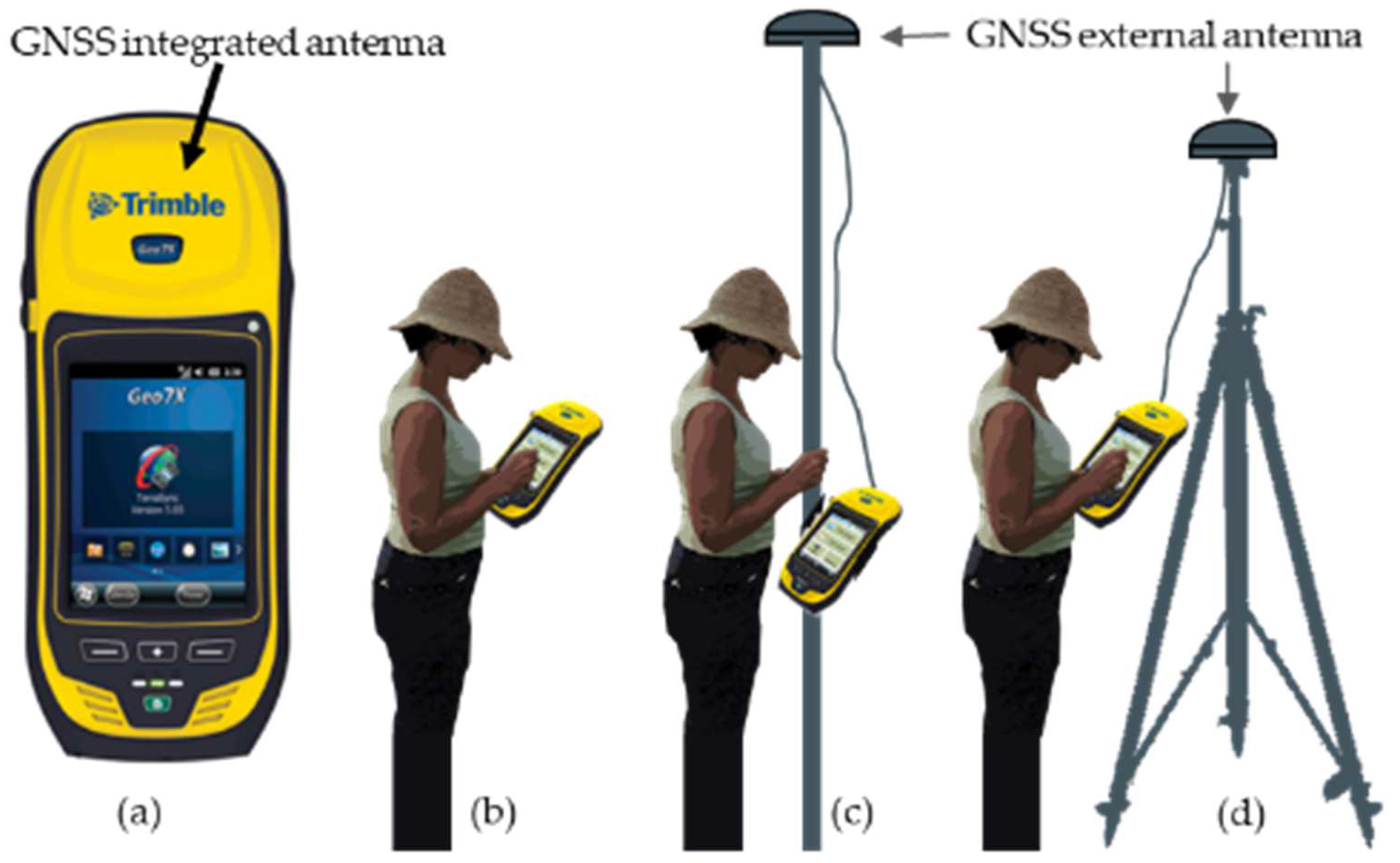
Figure 4.
Geo7x GNSS measurement accuracy in pole and tripod mode. (a) Pole mode with H the height of the antenna on the pole, α the inclination of the rod with respect to the vertical and D the distance between the tip of the pole and the vertical projection on the ground of the phase center of the antenna; (b) inclination of the rod of one degree results in a ground error of 3.5 cm; (c) tripod mode; (d) Leica GDF322 professional tribrach with optical plummet was used with the tripod for greater accuracy.
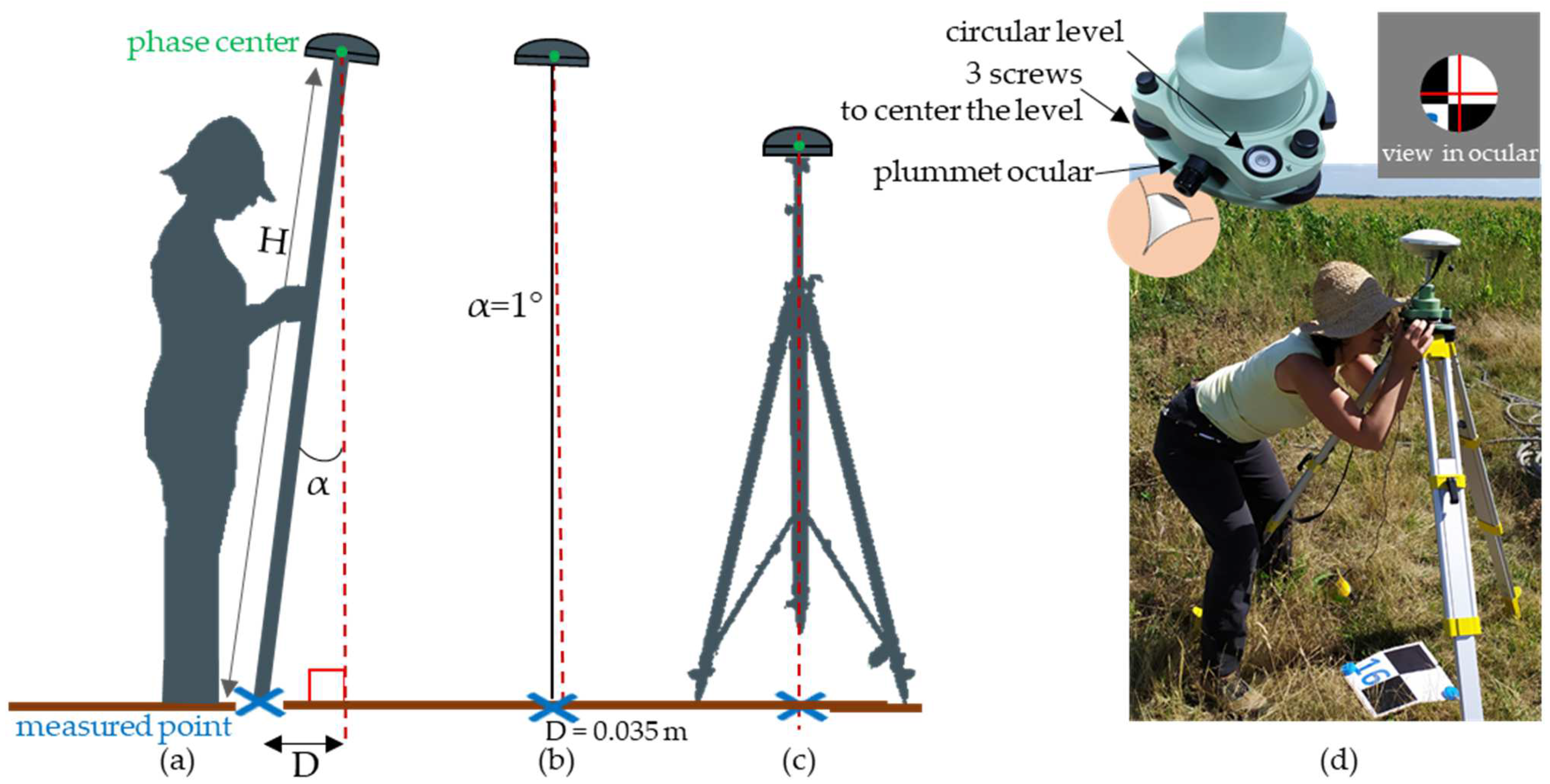
Figure 5.
Chavenay II GNSS station (RGP network).

Figure 6.
Measurement of the P4-RTK DGNSS receiver accuracy in static mode on the ground. (a) Two GCP, one for the D-RTK2 station and one for the P4-RTK; (b) P4-RTK GCP was a white wooden board, with a black cross in its center; (c) P4-RTK camera centered on its GCP; (d) remote controller screen, the black cross appeared in the GS RTK application (camera) and Custom Aim application created a red crosshair overlay in the center of the display, on top of the GS RTK application.
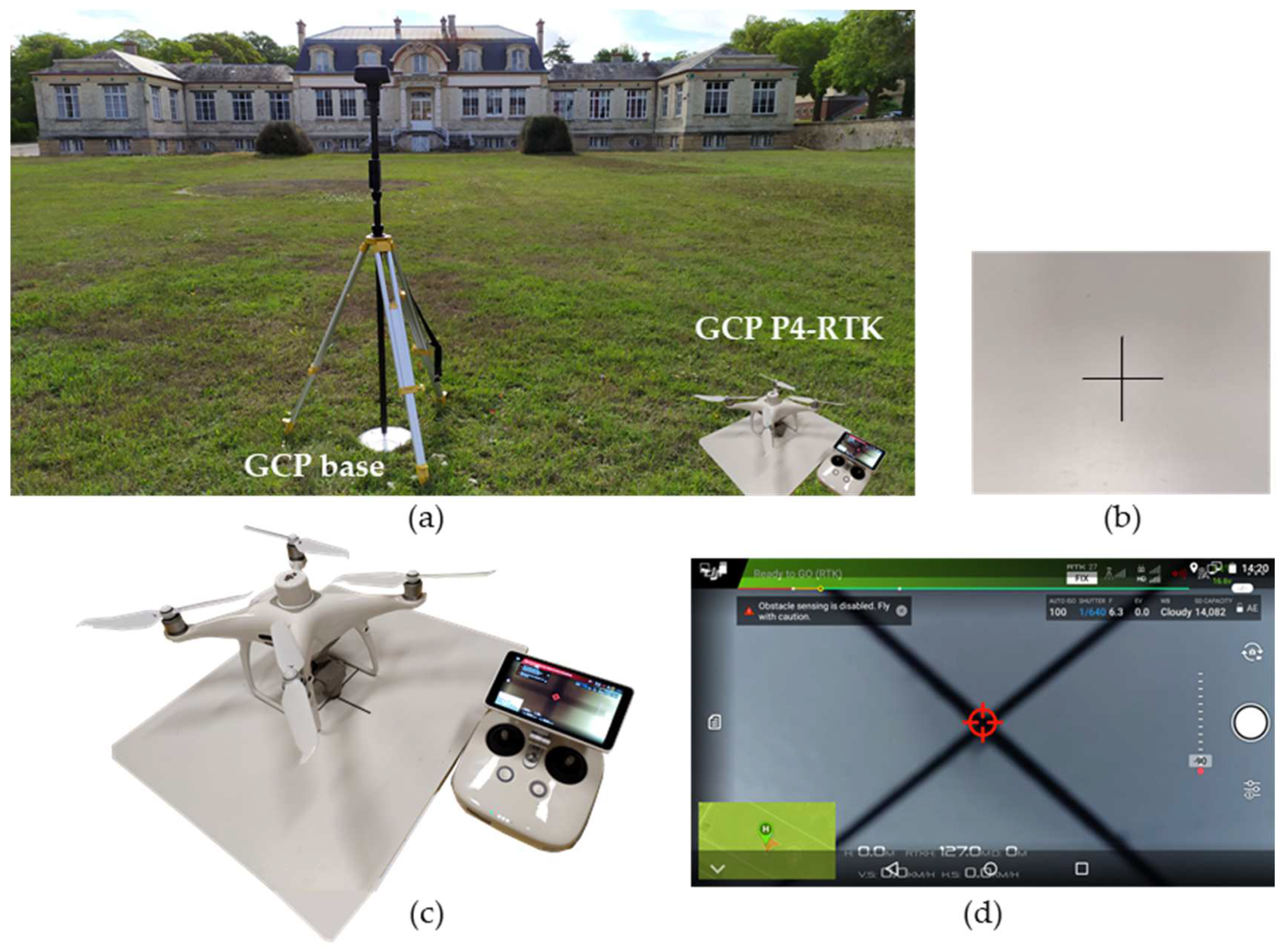
Figure 7.
Offset between the P4-RTK antenna phase center and its camera center.
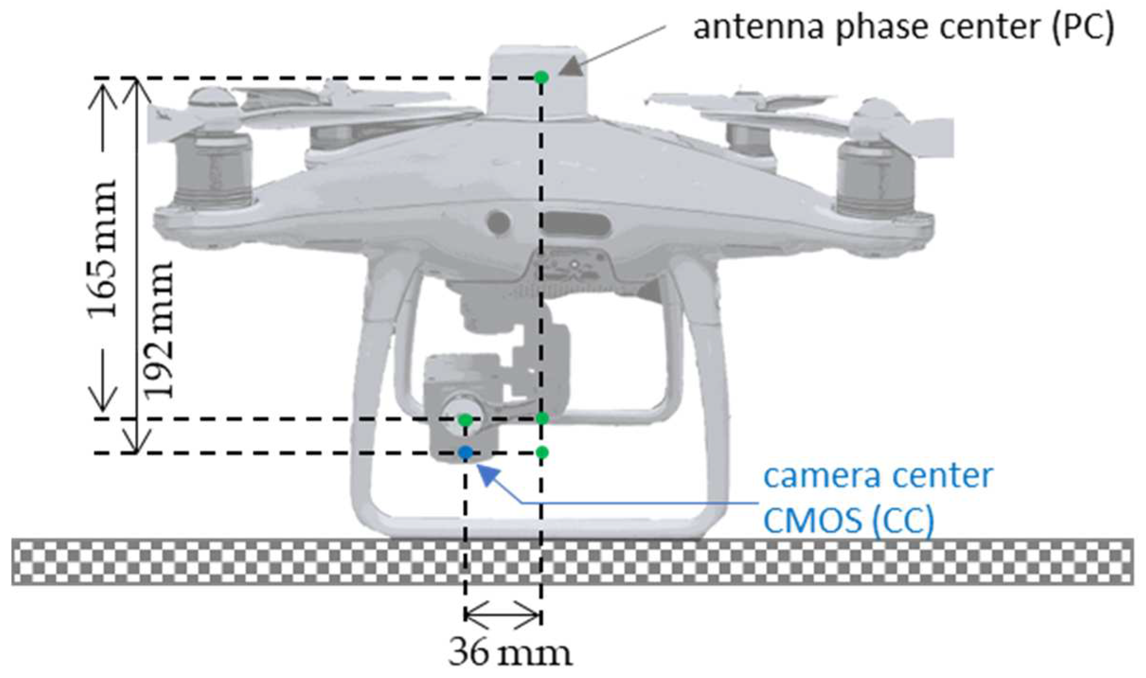
Figure 8.
Eight P4-RTK cardinal orientations, with ten repetitions each, to measure P4-RTK antenna accuracy on the ground.
Figure 8.
Eight P4-RTK cardinal orientations, with ten repetitions each, to measure P4-RTK antenna accuracy on the ground.
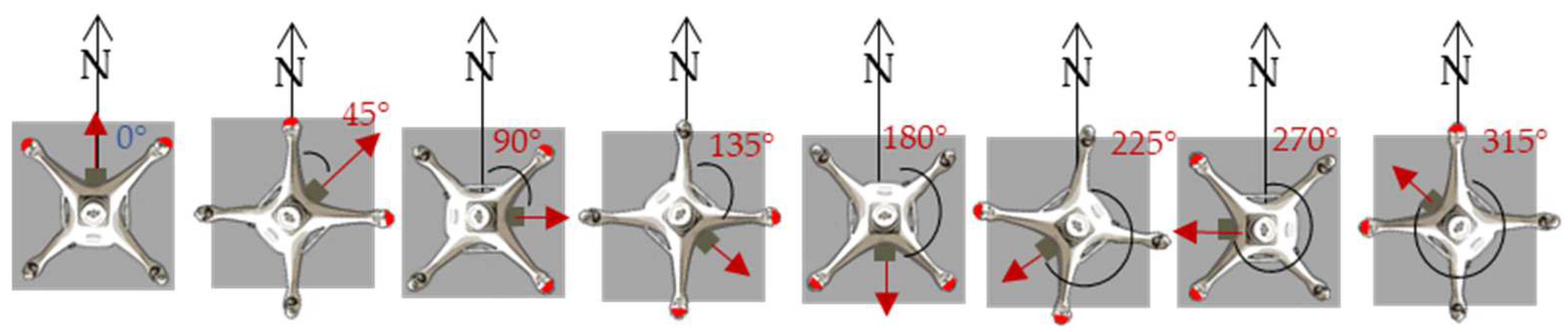
Figure 9.
GCPs used for the study. (a) Surveyor’s terminal as a reference point for the DRTK-2 base station; (b) semi-buried permanent GCP; (c) cardboard target as temporary GCP; (d) Geo7x terminal in tripod mode to measure GCPs position; (e) pPaper cone as a maize plant marker.
Figure 9.
GCPs used for the study. (a) Surveyor’s terminal as a reference point for the DRTK-2 base station; (b) semi-buried permanent GCP; (c) cardboard target as temporary GCP; (d) Geo7x terminal in tripod mode to measure GCPs position; (e) pPaper cone as a maize plant marker.

Figure 10.
Location in the study area of the 17 GCPs and 70 marked maize plants.
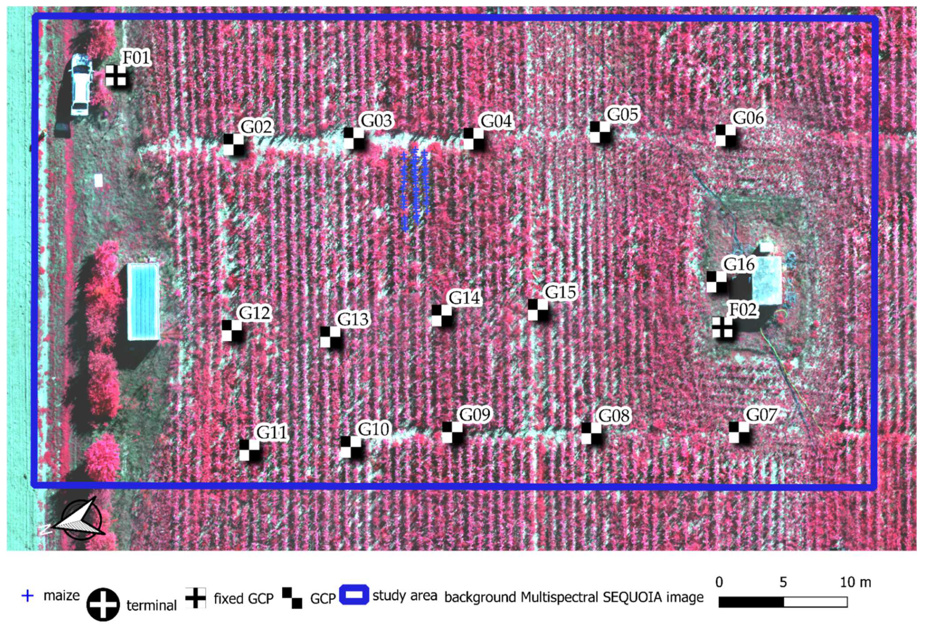
Figure 11.
Position of the 70 marked plants recorded with the Geo7x receiver in pole mode.
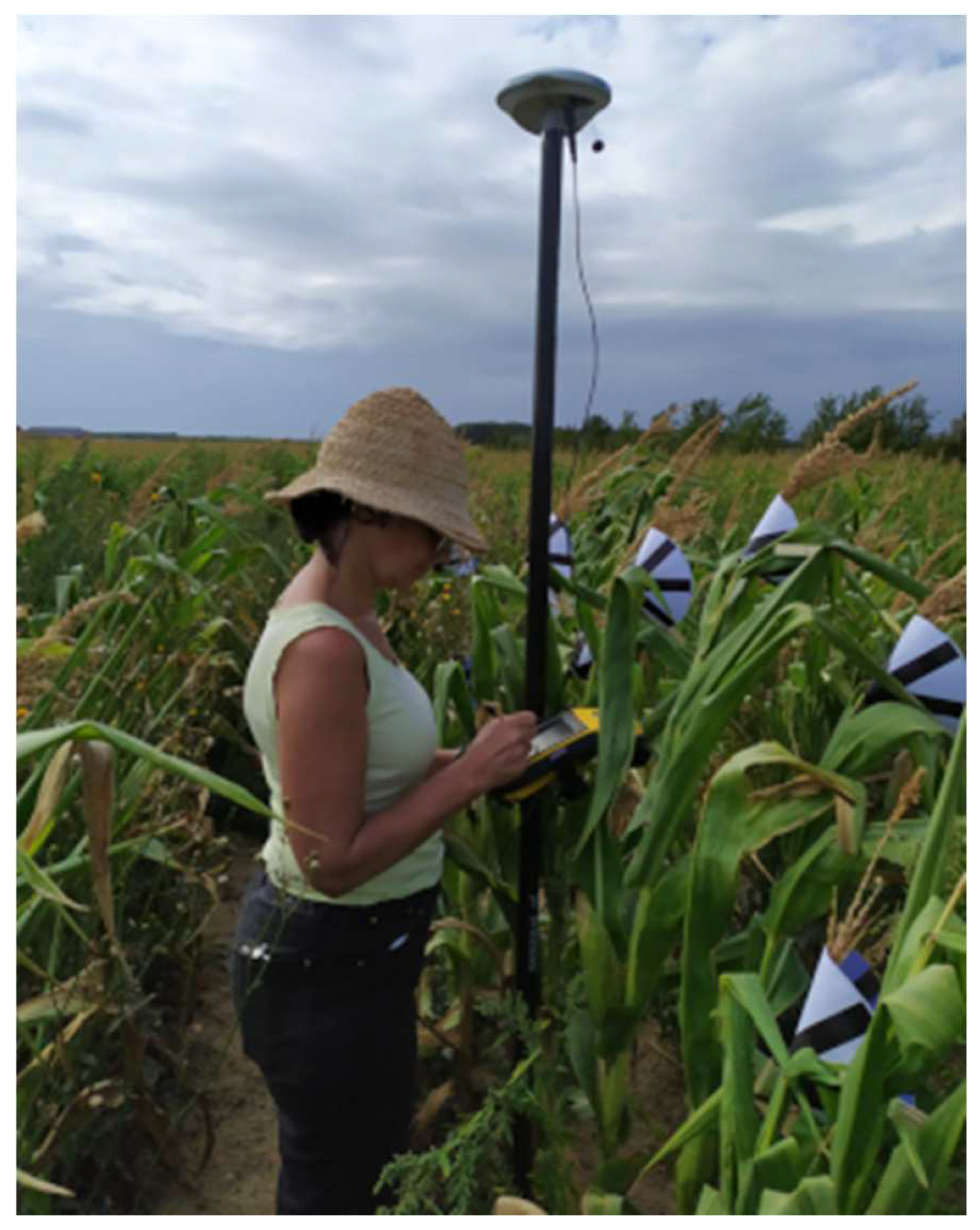
Figure 12.
Operating principle of D-RTK2 base station correction.

Figure 13.
Larger additional spirit level added to the D-RTK2 tripod.
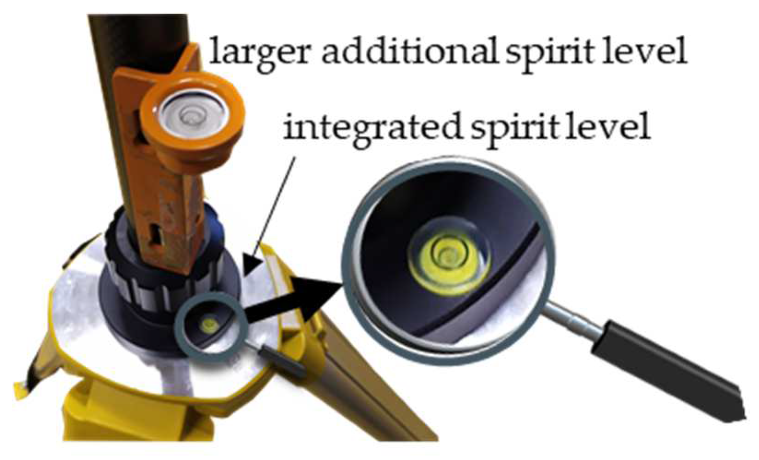
Figure 14.
Operating principle of the French Teria NRTK system.
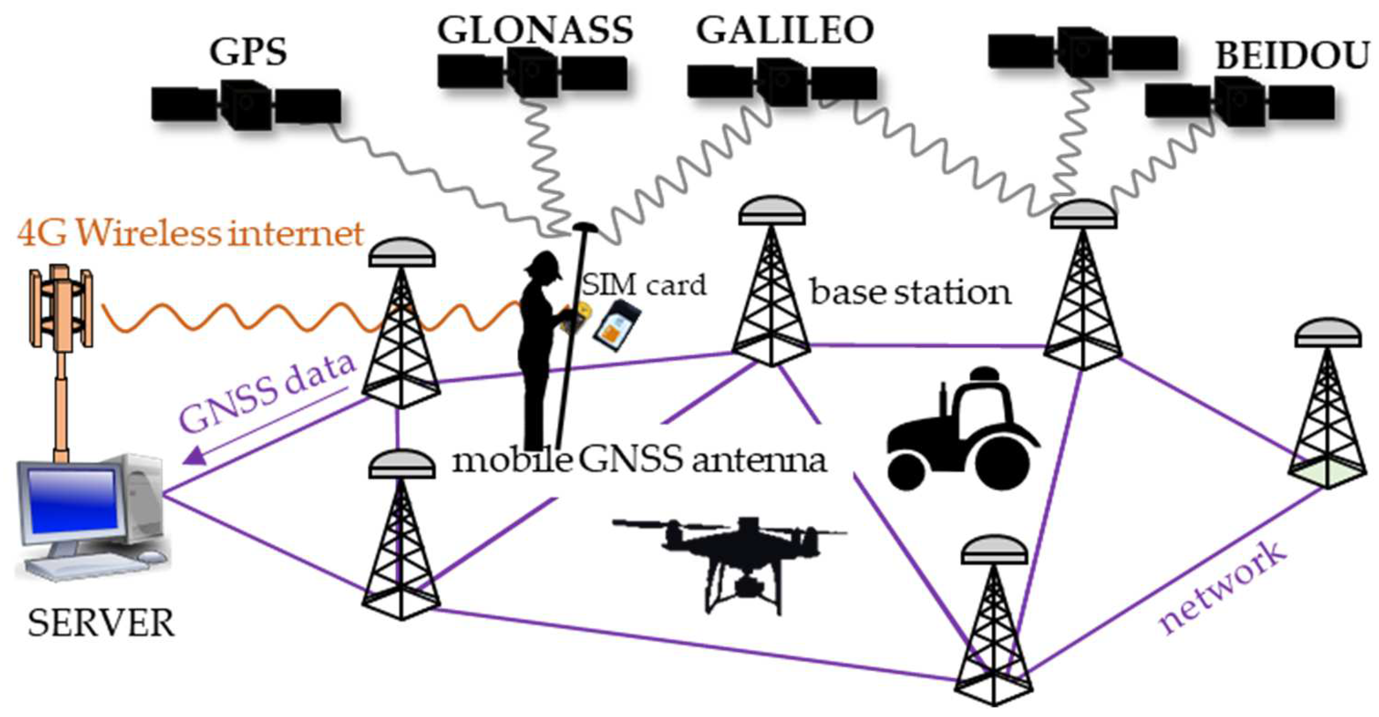
Figure 15.
Rinex observations file “100_0340_Rinex.obs” recorded during the GNSS mode flight of 27 August 2020 on the study area. Time of first and last observations.
Figure 15.
Rinex observations file “100_0340_Rinex.obs” recorded during the GNSS mode flight of 27 August 2020 on the study area. Time of first and last observations.
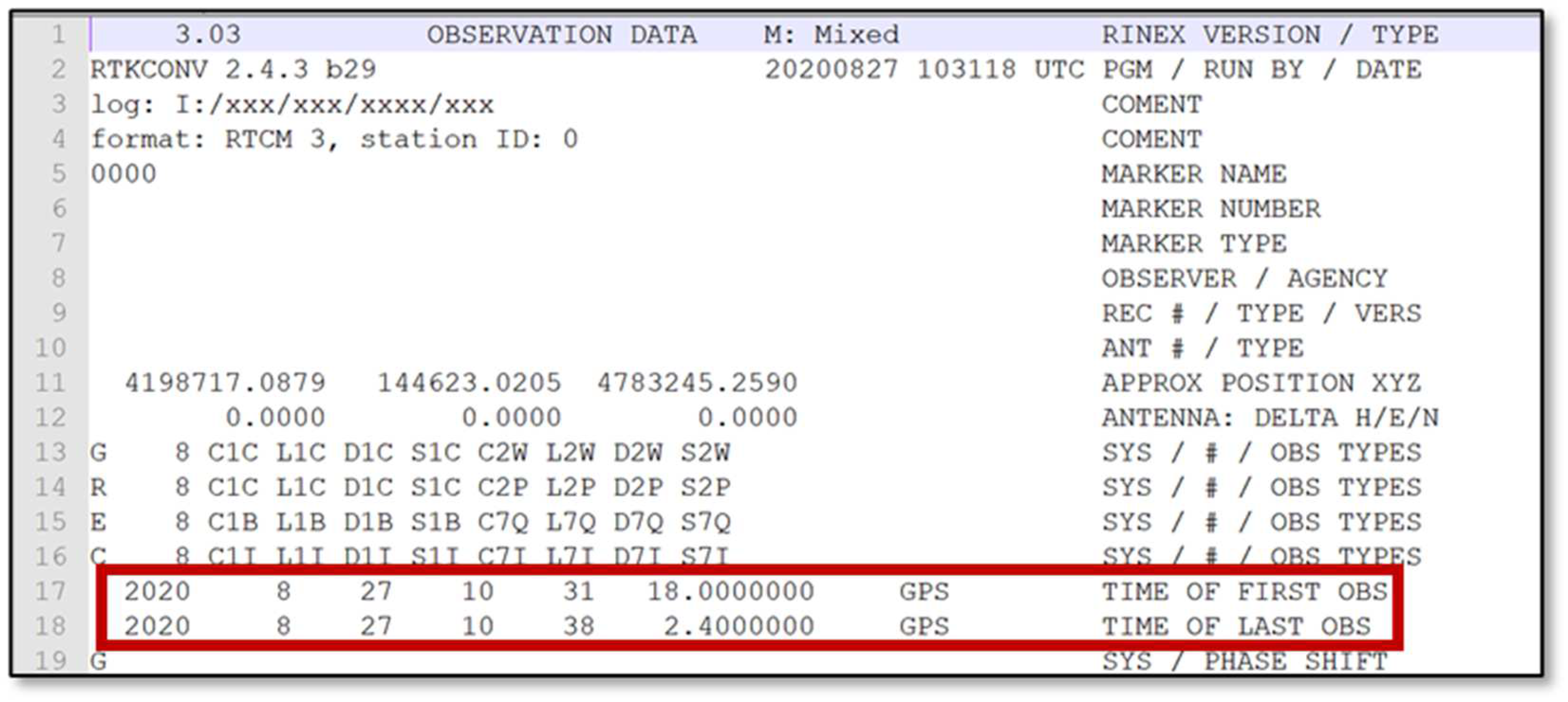
Figure 16.
Image position interpolation from Rinex observations. The two positions immediately before (B) and after (A) image capture were selected based on the time stamp. The trajectory was considered to be linear between two successive Rinex positions. The coefficient was used to determine the proximity of the image to the “before” and “after” point and was then used as a weighting coefficient for the calculation of the image latitude, longitude, and elevation from the two ppk positions.

Figure 17.
The P4-RTK attitude in flight (roll, pitch, yaw), the antenna phase center (PC), the P4-RTK gravity center (GC) and the SEQUOIA camera center (SC).
Figure 17.
The P4-RTK attitude in flight (roll, pitch, yaw), the antenna phase center (PC), the P4-RTK gravity center (GC) and the SEQUOIA camera center (SC).

Figure 18.
Flight path orientations used; (a) 194° direction for f1 reference flight; (b) 104° direction for flights f4 and f5.
Figure 18.
Flight path orientations used; (a) 194° direction for f1 reference flight; (b) 104° direction for flights f4 and f5.

Figure 19.
Image acquisition and photogrammetric processing. (a) Shooting of a couple of stereo images of a maize plant P, with, IP1 and IP2 the image plane of image 1 and 2 respectively, P1 and P2 the projections of point P in the two image planes, b the base and d the disparity; (b) photogrammetric processing workflow with Agisoft Metashape software.

Figure 20.
Overlap rate definitions: (a) forward overlap (vertical) side view; (b) GS RTK dialog box for overlapping choice; (c) forward overlap top view; (d) side overlap top view.
Figure 20.
Overlap rate definitions: (a) forward overlap (vertical) side view; (b) GS RTK dialog box for overlapping choice; (c) forward overlap top view; (d) side overlap top view.

Figure 21.
Location of GCPs used as control points for alignment in Metashape: (a) 1 GCP for reconstruction R_1_1gcp; (b) 3 GCPS for reconstruction R_1_3gcp; (c) 17 GCPs for reconstruction R_1_17gcp.
Figure 21.
Location of GCPs used as control points for alignment in Metashape: (a) 1 GCP for reconstruction R_1_1gcp; (b) 3 GCPS for reconstruction R_1_3gcp; (c) 17 GCPs for reconstruction R_1_17gcp.
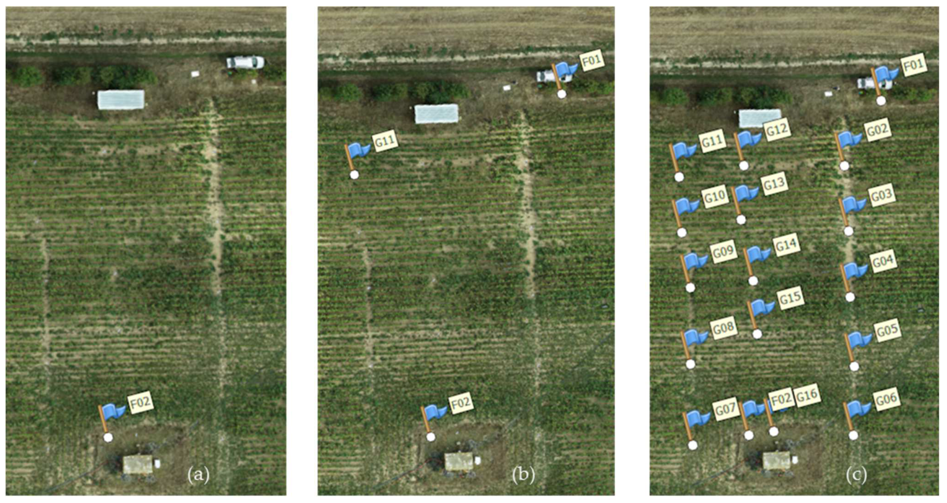
Figure 22.
GCP center (●) manually digitized from the ortho-image in a points layer using QGIS.
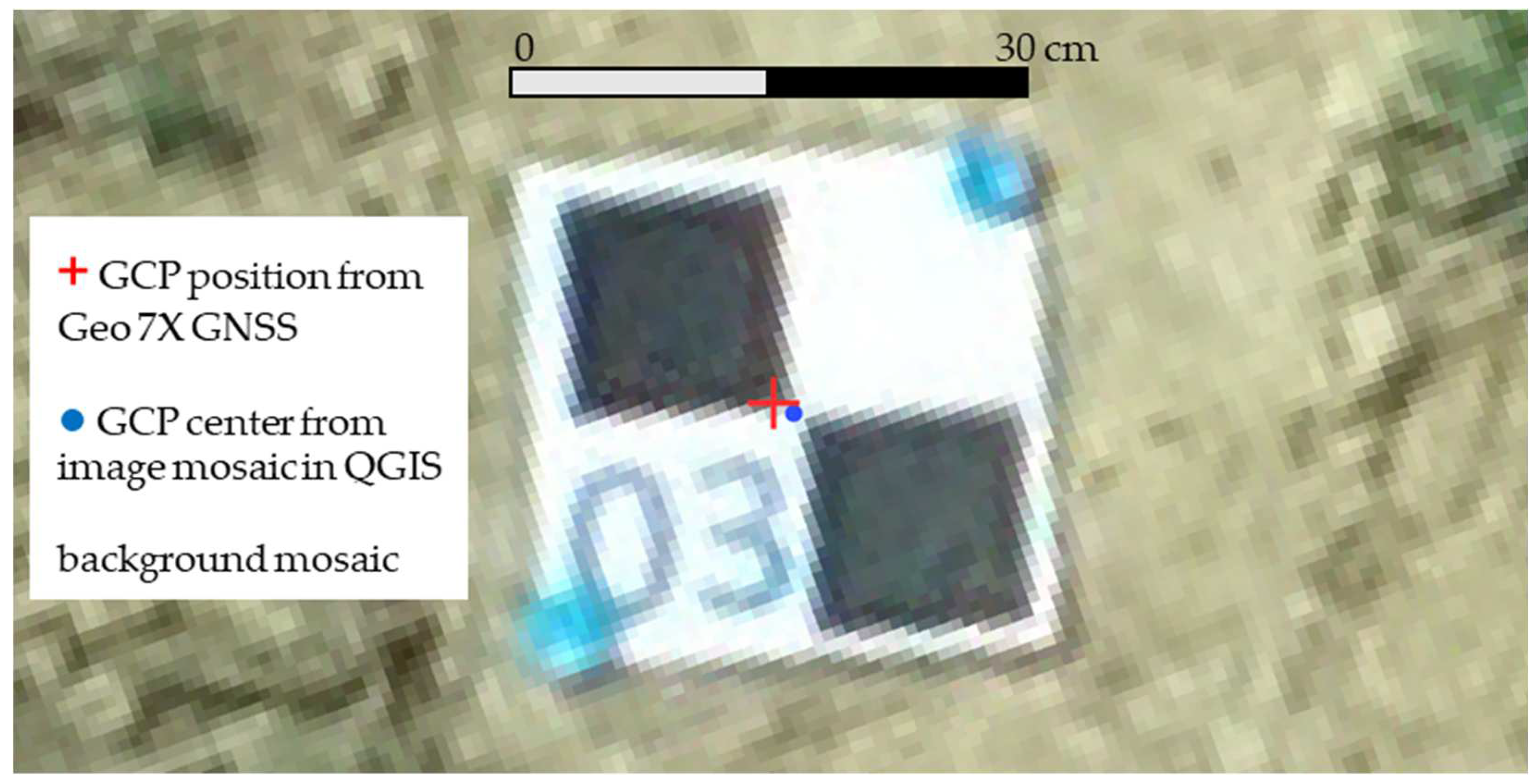
Figure 23.
Horizontal error (HE) and vertical error (VE) obtained on the basis of Trimble Geo7x GNSS receiver measurements on geodesic points in tripod and pole mode.
Figure 23.
Horizontal error (HE) and vertical error (VE) obtained on the basis of Trimble Geo7x GNSS receiver measurements on geodesic points in tripod and pole mode.

Figure 24.
Mean error on the X and Y coordinates of the GCP positions when using the P4-RTK antenna and the D-RTK2 station on the ground: (a) direct results; (b) results after centering on the global mean error.
Figure 24.
Mean error on the X and Y coordinates of the GCP positions when using the P4-RTK antenna and the D-RTK2 station on the ground: (a) direct results; (b) results after centering on the global mean error.
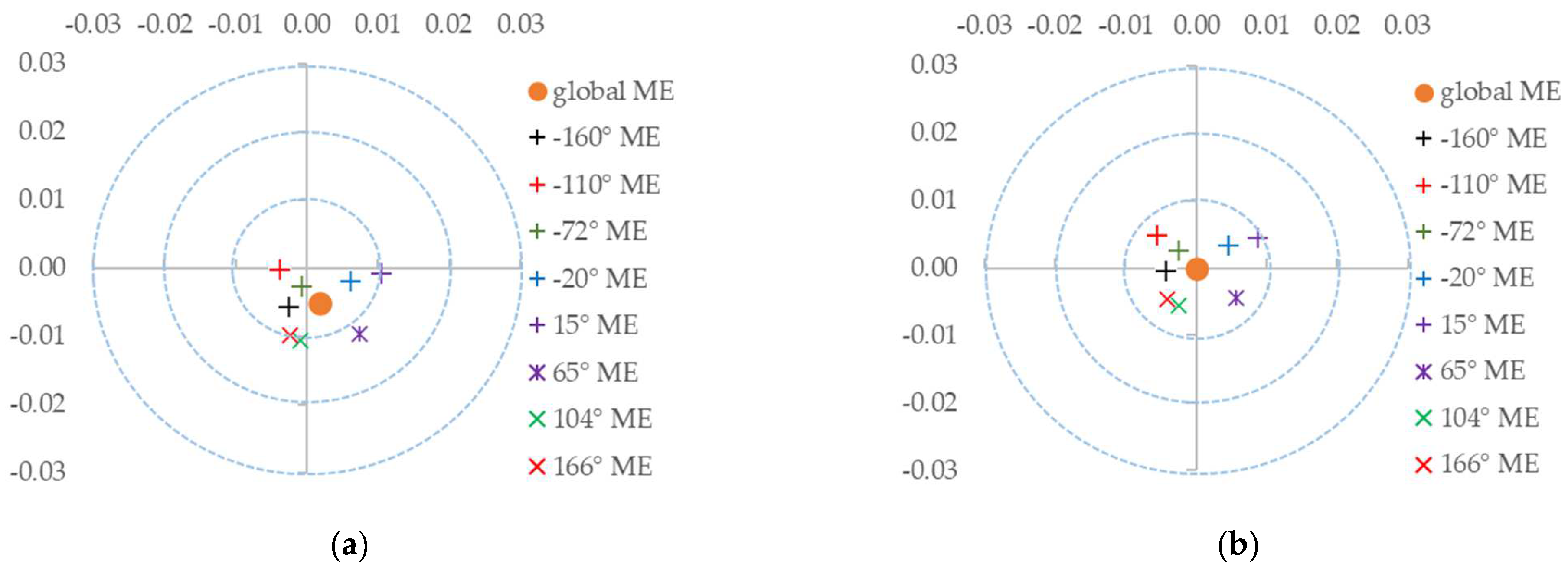
Figure 25.
Final ortho-mosaic of R_6 reconstruction, 14,633 × 17,119 pixels, 0.7 cm pixel resolution, at different scales: (a) Whole study area scale, 75 × 75 m; (b) medium scale, 25 × 25 m; (c) car scale, 7.5 × 7.5 m; (d) operator scale, 2.6 × 2.6 m.
Figure 25.
Final ortho-mosaic of R_6 reconstruction, 14,633 × 17,119 pixels, 0.7 cm pixel resolution, at different scales: (a) Whole study area scale, 75 × 75 m; (b) medium scale, 25 × 25 m; (c) car scale, 7.5 × 7.5 m; (d) operator scale, 2.6 × 2.6 m.
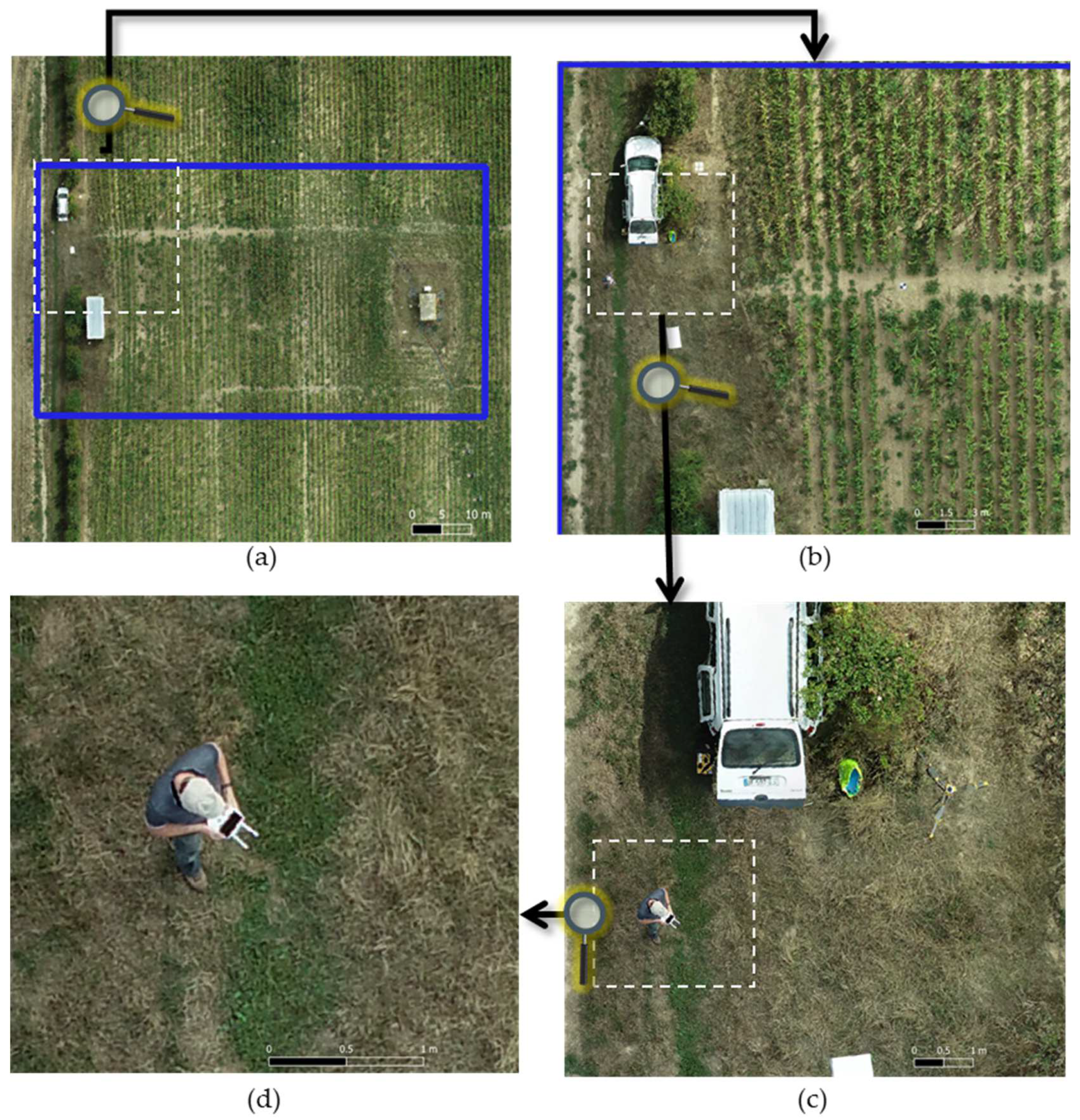
Figure 26.
Final ortho-mosaic of R_1 reconstruction, visualized in QGIS software, zoomed in on the 17 GCPs with an overlay of the GCP position measured on the ground using Geo7x DGNSS in tripod mode (●).
Figure 26.
Final ortho-mosaic of R_1 reconstruction, visualized in QGIS software, zoomed in on the 17 GCPs with an overlay of the GCP position measured on the ground using Geo7x DGNSS in tripod mode (●).
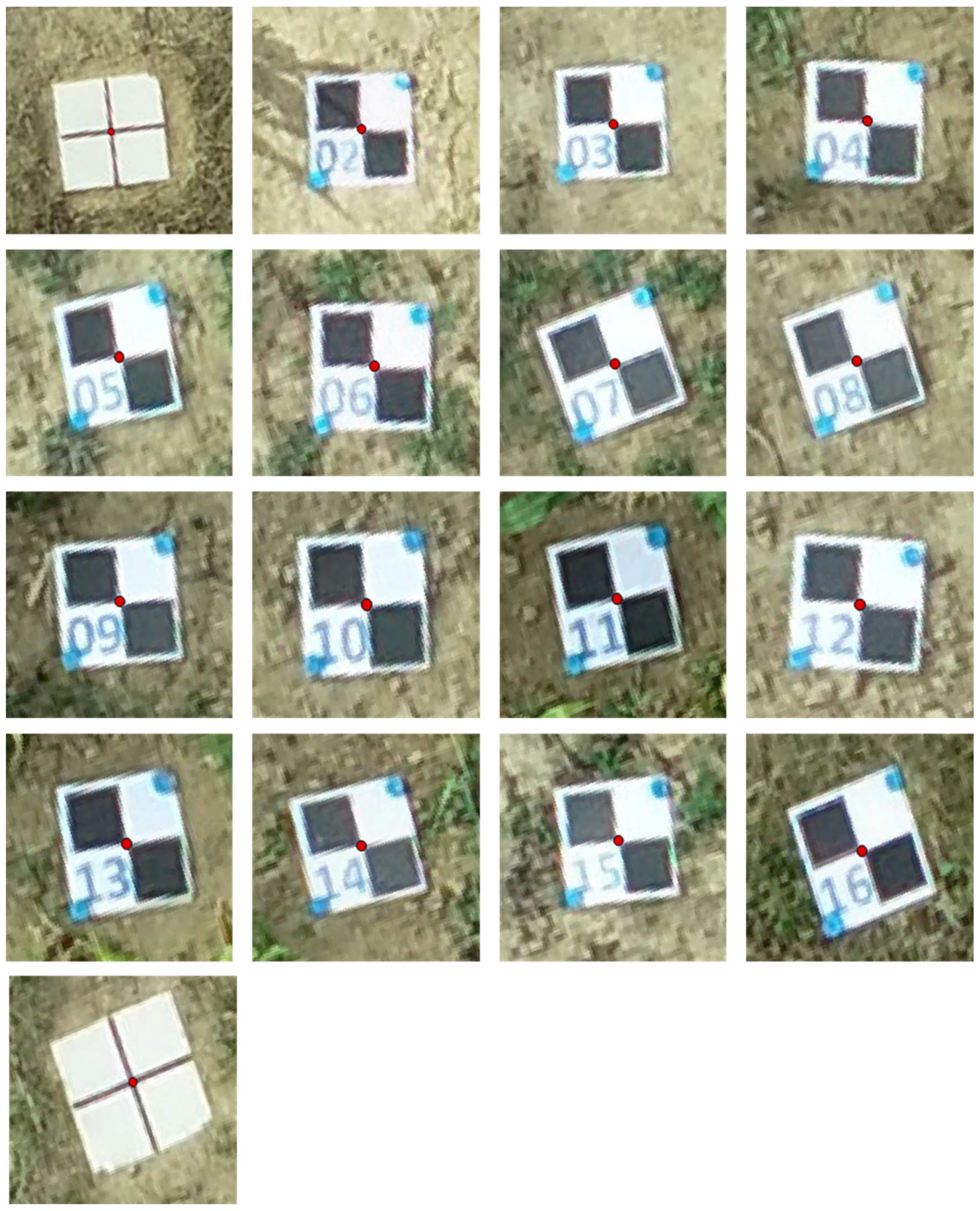
Figure 27.
Mean horizontal error (HE) calculated on the 17 GCPs for four GNSS modes.
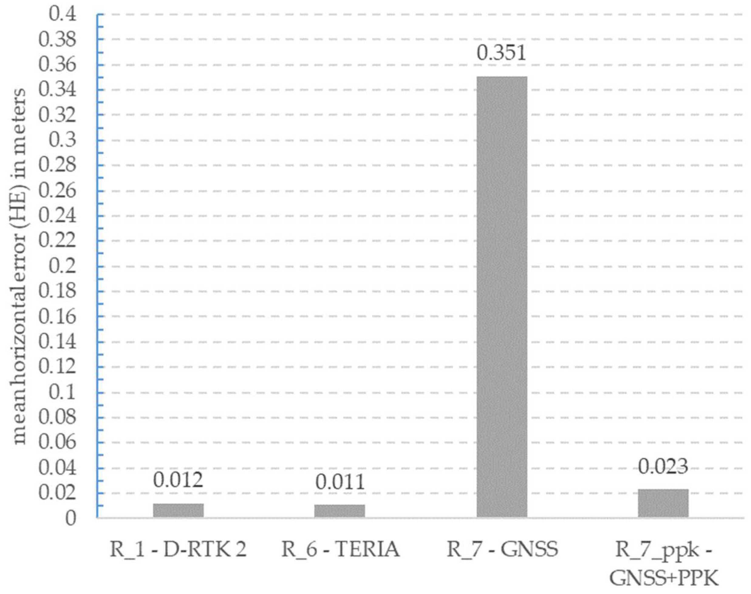
Figure 28.
Final ortho-mosaic of R_1 reconstruction, visualized in the QGIS software, zoom on the second maize row, with in overlay the plant positions, measured on the ground with Geo7x DGNSS in pole mode (+).
Figure 28.
Final ortho-mosaic of R_1 reconstruction, visualized in the QGIS software, zoom on the second maize row, with in overlay the plant positions, measured on the ground with Geo7x DGNSS in pole mode (+).
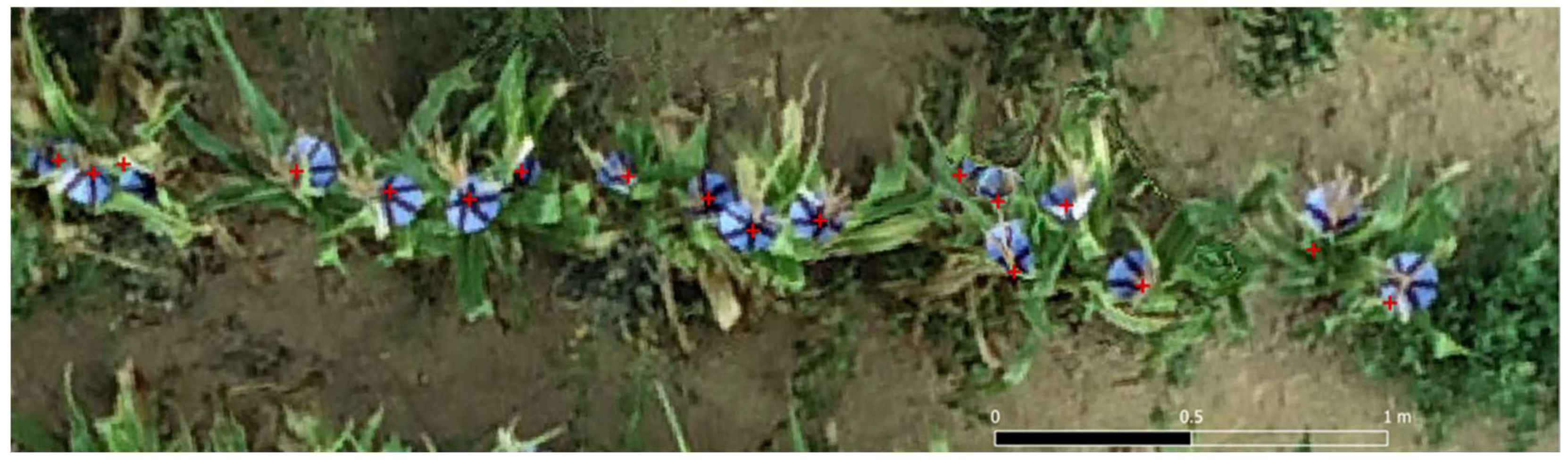
Figure 29.
Percentage of the 70 maize plants where HE ≤ distance, for each of the 12 reconstructions. (a) HE ≤ 5 cm; (b) HE ≤ 10 cm.
Figure 29.
Percentage of the 70 maize plants where HE ≤ distance, for each of the 12 reconstructions. (a) HE ≤ 5 cm; (b) HE ≤ 10 cm.
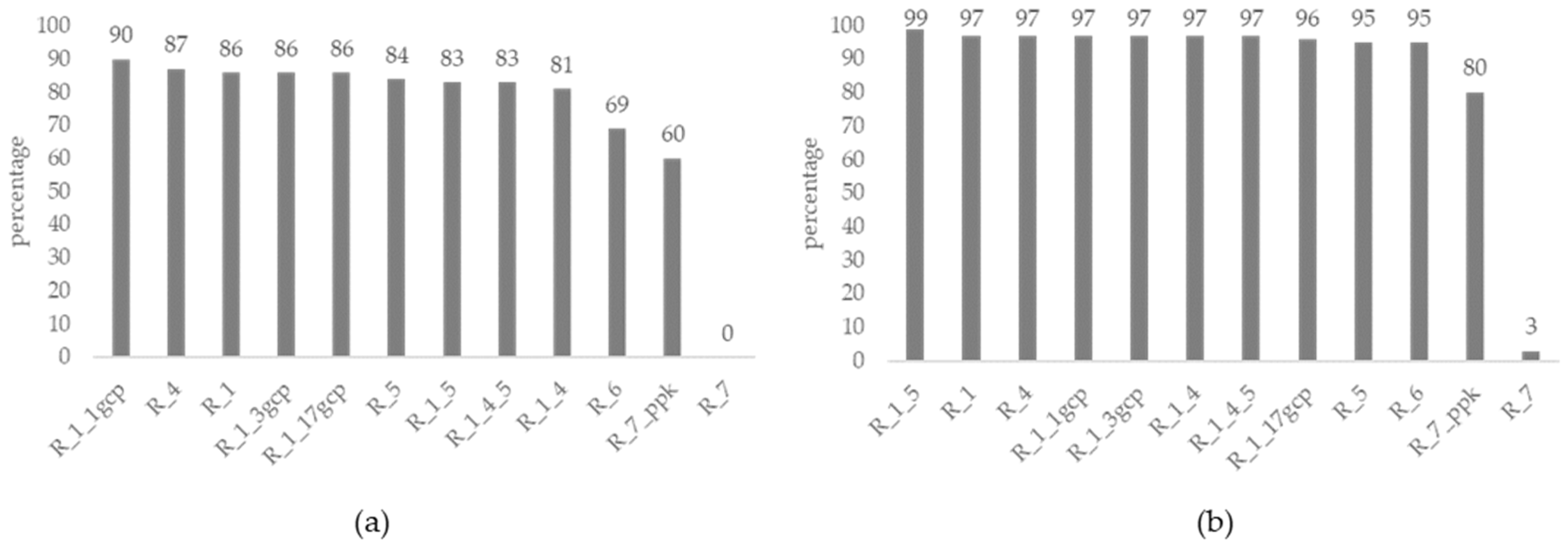
Table 1.
The main options used for the rtkpost software.
| Positioning Mode | Frequencies | Elevation Mask | Rec Dynamics | Solution Format | Time Format | Integer Ambiguity Res |
|---|---|---|---|---|---|---|
| Kinematic | L1 + L2 | 30° | OFF | Lat/lon/Height | ww ssss GPST | Fix and Hold |
Table 2.
Flight parameters used for the study.
| Fly | Date | Time UTC | AGL m | GSD m | Fly Direction ° | Overlap% Forward /Side | Speed m s−1 | Sat nb | GNSS Mode | Gimbal Angle | Sensors |
|---|---|---|---|---|---|---|---|---|---|---|---|
| f1 | 27 August 2020 | 9 h 3 | 25 | 0.007 | 194 | 80/70 | 1.8 | 18–21 | D-RTK2 | −90 | RGB |
| f4 | 27 August 2020 | 9 h 42 | 25 | 0.007 | 104 | 80/70 | 1.8 | 16–21 | D-RTK2 | −90 | RGB |
| f5 | 27 August 2020 | 9 h 57 | 40 | 0.011 | 104 | 80/70 | 1.8 | 18–20 | D-RTK2 | −90 | RGB |
| f6 | 27 August 2020 | 10 h 23 | 25 | 0.007 | 194 | 80/70 | 1.8 | 18–21 | TERIA | −90 | RGB |
| f7 | 27 August 2020 | 10 h 31 | 25 | 0.007 | 194 | 80/70 | 1.8 | 17–20 | GNSS | −90 | RGB |
Table 3.
The main parameter values for Agisoft Metashape v 1.7.4 reconstructions.
| Workflow Step | Parameter | Parameter Value |
|---|---|---|
| Add Photos | Camera accuracy (m) | 0.01 |
| Align Photos | Accuracy | High |
| Align Photos | Key point limit | 60,000 |
| Align Photos | Tie point limit | 0 (unlimited) |
| Optimize Camera Alignment | General | f, k1, k2, k3, cx, cy, p1, p2 |
| Optimize Camera Alignment | Advanced | Fit additional corrections |
| Build Dense Cloud | Quality | Mid |
| Build Dense Cloud | Depth filtering | Aggressive |
| Build DEM | Type | Geographic Lambert 93 |
| Build DEM | Source data | Dense cloud |
| Build DEM | Resolution (m) | 0.027 |
| Build Ortho-mosaic | Surface | DEM |
| Build Ortho-mosaic | Pixel size (m) | 0.007 |
| Build Ortho-mosaic | Refine seamlines | yes |
Table 4.
The 12 reconstructions that were computed with Agisoft Metashape.
| Metashape Reconstruction (R) | UAV Flights Used | GNSS Mode | GCP Used for Alignment | Camera Optimization |
|---|---|---|---|---|
| R_1 | f1 | D-RTK2 | 0 | yes |
| R_4 | f4 | D-RTK2 | 0 | yes |
| R_5 | f5 | D-RTK2 | 0 | yes |
| R_6 | f6 | TERIA | 0 | yes |
| R_7 | f7 | GNSS | 0 | yes |
| R_7_ppk | f7 | GNSS + PPK | 0 | yes |
| R_1_1gcp | f1 | D-RTK2 | 1 | yes |
| R_1_3gcp | f1 | D-RTK2 | 3 | yes |
| R_1_17gcp | f1 | D-RTK2 | 17 | yes |
| R_1_4 | f1 + f4 | D-RTK2 | 0 | yes |
| R_1_5 | f1 + f5 | D-RTK2 | 0 | yes |
| R_1_4_5 | f1 + f4 + f5 | D-RTK2 | 0 | yes |
Table 5.
Mean error (ME), root mean square error (RMSE), vertical error (VE) and horizontal error (HE) on X,Y,Z Chavenay II geodesic point coordinates, measured with a Trimble Geo7x GNSS receiver in tripod and pole mode. RGF93 Lambert 93 coordinate system.
Table 5.
Mean error (ME), root mean square error (RMSE), vertical error (VE) and horizontal error (HE) on X,Y,Z Chavenay II geodesic point coordinates, measured with a Trimble Geo7x GNSS receiver in tripod and pole mode. RGF93 Lambert 93 coordinate system.
| Mode | Positions Number | ME XL93 m | ME YL93 m | ME ZL93 m | RMSE XL93 m | RMSE YL93 m | VE ZL93 m | HE Distance m |
|---|---|---|---|---|---|---|---|---|
| tripod | 13 | −0.010 | −0.004 | −0.016 | 0.0097 | 0.0043 | 0.016 | 0.011 |
| pole | 32 | −0.030 | −0.030 | −0.041 | 0.0313 | 0.0306 | 0.042 | 0.043 |
Table 6.
Mean error (ME), root mean square error (RMSE), vertical error (VE) and horizontal error (HE) of GCP positions obtained using the P4-RTK antenna and the D-RTK2 station on the ground. Each line presents the average of 10 repetitions for one of the eight orientations of the drone; the last line presents the overall averages.
| Dir | ME XL93 m | ME YL93 m | ME ZL93 m | Pitch avg ° | Yaw avg ° | Roll avg ° | RMSE XL93 m | RMSE YL93 m | VE ZL93 m | HE Distance m |
|---|---|---|---|---|---|---|---|---|---|---|
| 1 | −0.003 | −0.006 | 0.004 | −0.28 | −161 | −0.20 | 0.003 | 0.006 | 0.006 | 0.006 |
| 2 | −0.004 | 0.000 | −0.005 | 0.01 | −110 | 0.11 | 0.004 | 0.004 | 0.007 | 0.004 |
| 3 | −0.001 | −0.003 | −0.003 | 0.00 | −72 | 0.58 | 0.001 | 0.003 | 0.007 | 0.003 |
| 4 | 0.006 | −0.002 | −0.008 | −0.30 | −20 | 1.00 | 0.006 | 0.003 | 0.010 | 0.007 |
| 5 | 0.010 | −0.001 | 0.003 | −0.70 | 15 | 1.10 | 0.011 | 0.002 | 0.005 | 0.011 |
| 6 | 0.007 | −0.010 | 0.000 | −1.20 | 65 | 0.67 | 0.007 | 0.010 | 0.004 | 0.012 |
| 7 | −0.001 | −0.011 | 0.002 | −1.20 | 104 | 0.20 | 0.002 | 0.011 | 0.004 | 0.011 |
| 8 | −0.002 | −0.010 | −0.002 | −0.68 | 166 | −0.30 | 0.003 | 0.010 | 0.005 | 0.010 |
| avg | 0.002 | −0.005 | −0.001 | −0.54 | −1.77 | 0.40 | 0.005 | 0.006 | 0.006 | 0.008 |
Table 7.
The 12 photogrammetric reconstruction output parameters.
| R | Cameras Number | Sparse Cloud Points | Dense Cloud Points | Ortho-Mosaic Size pixels | Ortho-Mosaic Resolution m | MNS Size Pixels | MNS Resolution m |
|---|---|---|---|---|---|---|---|
| R_1 | 168 | 291,514 | 25,536,868 | 17,116 × 19,046 | 0.007 | 5217 × 5955 | 0.027 |
| R_4 | 116 | 189,291 | 19,547,225 | 14,435 × 17,536 | 0.007 | 4093 × 5103 | 0.028 |
| R_6 | 109 | 182,361 | 17,295,530 | 14,633 × 17,119 | 0.007 | 4079 × 5010 | 0.027 |
| R_5 | 35 | 65,611 | 7,811,874 | 9876 × 12,272 | 0.011 | 2644 × 3462 | 0.043 |
| R_7 | 147 | 266,433 | 22,460,812 | 15,146 × 18,520 | 0.007 | 4286 × 5469 | 0.027 |
| R_7_ppk | 147 | 266,698 | 22,575,332 | 15,446 × 19,004 | 0.007 | 4279 × 5464 | 0.027 |
| R_1_1gcp | 168 | 291,637 | 25,507,163 | 17,113 × 19,043 | 0.007 | 5217 × 5954 | 0.027 |
| R_1_3gcp | 168 | 312,033 | 25,296,142 | 11,981 × 13,331 | 0.007 | 5139 × 5905 | 0.027 |
| R_1_17gcp | 168 | 312,033 | 25,296,142 | 11,981 × 13,331 | 0.010 | 5139 × 5905 | 0.027 |
| R_1_4 | 284 | 669,304 | 28,055,902 | 16,745 × 18,910 | 0.007 | 4610 × 5386 | 0.027 |
| R_1_5 | 203 | 365,795 | 21,569,171 | 17,320 × 19,787 | 0.007 | 4675 × 5404 | 0.029 |
| R_1_4_5 | 319 | 745,453 | 25,554,817 | 16,981 × 19,165 | 0.007 | 4388 × 5120 | 0.029 |
Table 8.
Horizontal (HE) and vertical error (VE) statistics for GCP positions for the 12 reconstructions.
Table 8.
Horizontal (HE) and vertical error (VE) statistics for GCP positions for the 12 reconstructions.
| R | GNSS Mode | HE Mean | HE sd | HE Min | HE Max | VE Mean | VE sd | VE Min | VE Max |
|---|---|---|---|---|---|---|---|---|---|
| R_1 | D-RTK2 | 0.012 | 0.006 | 0.002 | 0.021 | 0.029 | 0.018 | 0.000 | 0.064 |
| R_4 | D-RTK2 | 0.012 | 0.005 | 0.004 | 0.021 | 0.023 | 0.019 | 0.001 | 0.067 |
| R_5 | D-RTK2 | 0.016 | 0.007 | 0.004 | 0.028 | 0.067 | 0.028 | 0.025 | 0.12 |
| R_6 | TERIA | 0.011 | 0.005 | 0.001 | 0.022 | 0.032 | 0.019 | 0.004 | 0.064 |
| R_7 | GNSS | 0.351 | 0.162 | 0.059 | 0.709 | 1.043 | 0.129 | 0.735 | 1.192 |
| R_7_ppk | GNSS PPK | 0.023 | 0.007 | 0.008 | 0.035 | 0.097 | 0.029 | 0.050 | 0.148 |
| R_1_1gcp | D-RTK2 | 0.012 | 0.006 | 0.002 | 0.021 | 0.020 | 0.016 | 0.002 | 0.056 |
| R_1_3gcp | D-RTK2 | 0.011 | 0.006 | 0.002 | 0.021 | 0.017 | 0.014 | 0.001 | 0.049 |
| R_1_17gcp | D-RTK2 | 0.011 | 0.005 | 0.001 | 0.021 | 0.017 | 0.014 | 0.002 | 0.047 |
| R_1_4 | D-RTK2 | 0.012 | 0.006 | 0.002 | 0.021 | 0.034 | 0.021 | 0.000 | 0.074 |
| R_1_5 | D-RTK2 | 0.012 | 0.006 | 0.002 | 0.021 | 0.020 | 0.014 | 0.001 | 0.045 |
| R_1_4_5 | D-RTK2 | 0.013 | 0.006 | 0.003 | 0.021 | 0.021 | 0.013 | 0.003 | 0.050 |
Table 9.
Horizontal error (HE) statistics on maize plant position for the 12 reconstructions. The percentages represent the percentage of the maize plant population for which the horizontal error is in a distance interval.
Table 9.
Horizontal error (HE) statistics on maize plant position for the 12 reconstructions. The percentages represent the percentage of the maize plant population for which the horizontal error is in a distance interval.
| R | GNSS Mode | HE Mean | HE sd | HE Min | HE Max | % HE <5 cm | % HE 5–10 cm | % HE >10 cm |
|---|---|---|---|---|---|---|---|---|
| R_1 | D-RTK2 | 0.019 | 0.030 | 0.000 | 0.152 | 86 | 11 | 3 |
| R_4 | D-RTK2 | 0.030 | 0.044 | 0.000 | 0.264 | 87 | 10 | 3 |
| R_5 | D-RTK2 | 0.032 | 0.034 | 0.000 | 0.176 | 84 | 11 | 4 |
| R_6 | TERIA | 0.040 | 0.035 | 0.000 | 0.163 | 69 | 26 | 6 |
| R_7 | GNSS | 0.257 | 0.055 | 0.065 | 0.391 | 0 | 3 | 97 |
| R_7_ppk | GNSS PPK | 0.054 | 0.052 | 0.000 | 0.185 | 60 | 20 | 20 |
| R_1_1gcp | D-RTK2 | 0.020 | 0.029 | 0.000 | 0.172 | 90 | 7 | 3 |
| R_1_3gcp | D-RTK2 | 0.020 | 0.028 | 0.000 | 0.148 | 86 | 11 | 3 |
| R_1_17gcp | D-RTK2 | 0.024 | 0.034 | 0.000 | 0.182 | 86 | 10 | 4 |
| R_1_4 | D-RTK2 | 0.025 | 0.031 | 0.000 | 0.157 | 81 | 16 | 3 |
| R_1_5 | D-RTK2 | 0.026 | 0.029 | 0.000 | 0.152 | 83 | 16 | 1 |
| R_1_4_5 | D-RTK2 | 0.027 | 0.029 | 0.000 | 0.152 | 83 | 14 | 3 |
Publisher’s Note: MDPI stays neutral with regard to jurisdictional claims in published maps and institutional affiliations. |
© 2022 by the authors. Licensee MDPI, Basel, Switzerland. This article is an open access article distributed under the terms and conditions of the Creative Commons Attribution (CC BY) license (https://creativecommons.org/licenses/by/4.0/).
Share and Cite
MDPI and ACS Style
Gilliot, J.-M.; Hadjar, D.; Michelin, J. Potential of Ultra-High-Resolution UAV Images with Centimeter GNSS Positioning for Plant Scale Crop Monitoring. Remote Sens. 2022, 14, 2391. https://doi.org/10.3390/rs14102391
AMA Style
Gilliot J-M, Hadjar D, Michelin J. Potential of Ultra-High-Resolution UAV Images with Centimeter GNSS Positioning for Plant Scale Crop Monitoring. Remote Sensing. 2022; 14(10):2391. https://doi.org/10.3390/rs14102391
Chicago/Turabian StyleGilliot, Jean-Marc, Dalila Hadjar, and Joël Michelin. 2022. "Potential of Ultra-High-Resolution UAV Images with Centimeter GNSS Positioning for Plant Scale Crop Monitoring" Remote Sensing 14, no. 10: 2391. https://doi.org/10.3390/rs14102391
Note that from the first issue of 2016, this journal uses article numbers instead of page numbers. See further details here.