
PlanetScope, Sentinel-2, and Sentinel-1 Data Integration for Object-Based Land Cover Classification in Google Earth Engine


Department of Agricultural, Food and Environmental Sciences, University of Perugia, 06121 Perugia, Italy
Remote Sens. 2022, 14(11), 2628; https://doi.org/10.3390/rs14112628
Submission received: 6 April 2022
/
Revised: 25 May 2022
/
Accepted: 29 May 2022
/
Published: 31 May 2022
(This article belongs to the Special Issue Remote Sensing of Land Use and Land Change with Google Earth Engine)
Abstract
:PlanetScope (PL) high-resolution composite base maps have recently become available within Google Earth Engine (GEE) for the tropical regions thanks to the partnership between Google and the Norway’s International Climate and Forest Initiative (NICFI). Object-based (OB) image classification in the GEE environment has increased rapidly due to the broadly recognized advantages of applying these approaches to medium- and high-resolution images. This work aimed to assess the advantages for land cover classification of (a) adopting an OB approach with PL data; and (b) integrating the PL datasets with Sentinel 2 and Sentinel 1 data both in Pixel-based (PB) or OB approaches. For this purpose, in this research, we compared ten LULC classification approaches (PB and OB, all based on the Random Forest (RF) algorithm), where the three satellite datasets were used according to different levels of integration and combination. The study area, which is 69,272 km2 wide and located in central Brazil, was selected within the tropical region, considering a preliminary availability of sample points and its complex landscape mosaic composed of heterogeneous agri-natural spaces, including scattered settlements. Using only the PL dataset with a typical RF PB approach produced the worse overall accuracy (OA) results (67%), whereas adopting an OB approach for the same dataset yielded very good OA (82%). The integration of PL data with the S2 and S1 datasets improved both PB and OB overall accuracy outputs (82 vs. 67% and 91 vs. 82%, respectively). Moreover, this research demonstrated the OB approaches’ applicability in GEE, even in vast study areas and using high-resolution imagery. Although additional applications are necessary, the proposed methodology appears to be very promising for properly exploiting the potential of PL data in GEE.
1. Introduction
Satellite remote sensing (RS) offers critical information for mapping and understanding our planet’s surface. RS-derived geo-information has been extensively used to address relevant topics in tropical areas such as deforestation, biomass estimation, biodiversity loss, and drought [1], and their impacts on rural communities, soils, vegetation, wildlife, watersheds, and global warming climatic trends [2]. The creation of land use/land cover (LULC) maps, which depict how land is utilized for various human purposes or the physical properties of the Earth’s surface, is a typical RS data use [3]. LULC maps offer critical information for studying landscape composition and configuration, and identifying changes in the landscape along its LULC gradients [4,5]. Understanding LULC changes and locating transformation hotspots are crucial for ecosystem monitoring, protection, and management [6,7].
RS data archives are constantly expanding, with rising satellite availability and image resolutions (radiometric, spectral, spatial, temporal), allowing users to potentially access and study massive time-series datasets, but with increasing time and computing costs. In recent years, RS data processing has shifted from traditional workstations with cutting-edge, often costly hardware and RS software, to cloud-based platforms. The latter enable users to instantly access and analyze pre-processed geospatial data via user-friendly, web-based interfaces and powerful scripting languages [8]. Among these systems, Google Earth Engine (GEE) is a cloud-based geospatial analytic platform that allows users to tackle the fundamental difficulties of managing enormous volumes of data, and their storage, processing, and analysis in a highly effective manner [9].
The recent partnership between Google and Norway’s International Climate and Forest Initiative (NICFI) has led to the addition of NICFI PlanetScope Basemaps (700+ geospatial high resolution, 4.77 m, datasets) to GEE’s public data catalog [10]. These datasets provide broad time series (December 2015–August 2020, biannual; September 2020 onward, monthly), four-band (RGB+NIR), and coverage of 94 countries across the global tropics [11]. The availability of PlanetScope (PL) data within GEE is an important step forward for detecting and monitoring LULC dynamics at high resolution, including small-scale disturbances, in tropical landscapes.
Ordinary LULC automated classification algorithms for RS data use training data to build spectral signatures of selected LULC classes and pixel-based (PB) discrimination between selected classes using more or less advanced classification algorithms [12,13]. Object-based (OB) approaches (so-called GEographic Object-Based Image Analysis—GEOBIA) have become more popular due to their capability to delineate and classify landscape objects or patches at different scales [14,15,16]. An essential stage in object delineation is pixel clustering and segmentation, aiming to combine comparable pixels into image clusters and transform them into vectors [17,18]. Despite the increased processing cost of segmentation and numerous features for classification, OB approaches often yield better results for higher resolution data, whereas the PB approach is generally suggested for lower image resolutions [19]. OB classification processes, usually performed within specific, often proprietary, image processing software [20], can also be successfully implemented in GEE [16,21]. In this environment, the Simple Non-Iterative Clustering (SNIC) method has been proven to be particularly effective in similar grouping pixels and identifying probable unique objects or landscape patches. SNIC was successfully applied using high-resolution images [18,19] or medium-resolution satellite data, such as Landsat [16,22]. Following image clustering, GEOBIA performs object categorization by combining spectral and geographical information with the texture and context information of the image [21,23]. The Gray-Level Co-occurrence Matrix (GLCM) can be used in GEE to extract the objects’ textural indices that represent additional information used in the classification [21,24]. The OB approach has been effectively implemented in GEE for various applications: crop mapping in the Sanjiang plain, China, using S2 data and combined growth-period attributes [25]; LULC classification and analysis of the Munneru River Basin, India [26]; and crop classification in the Heilongjiang province, China, using Sentinel-1 time series [27].
In the classification of LULC, non-parametric machine learning (ML) techniques generally yield better results than standard classifiers since they do not need hypotheses about the input data distribution. Among the various ML classifiers, the Classification and Regression Tree (CART) is a binary decision tree classifier that employs a predetermined threshold [13], while Random Forest (RF) is an ensemble classifier that uses multiple CART [28]. The latter is one of the most effective, accurate, and broadly used classifiers used for LULC classification [29]. The Support Vector Machine (SVM) is also an excellent classifier, but its application is more challenging since it needs the definition of essential input parameters as the kernel type [30]. RF is the most extensively used ML method in the GEE context [31] and, in general, for remote sensing data categorization [32,33]. This is due to its non-parametric nature, ability to manage dimensionality and overfitting, and excellent performance compared to other classifiers. RF is based on numerous CARTs, with their average used to make the final classification. One of its most significant inherent weaknesses is the unknown splitting rules [34].
Integrating satellite data from different sensors is a common approach in RS science [35,36]. Sentinel-2 (S2) and Sentinel-1 (S1) data have been often combined to improve the accuracy of LULC classification [37,38,39], and also integrated with Landsat 8 data [40,41]. PL imagery has previously been combined with S2 and S1 in PB land cover classification approaches for crop mapping of smallholder farms in eastern India using SVM [42], and crop and LULC mapping in Northern Malawi, using RF within GEE [43]. The former achieved the highest accuracies when using the model that included all three sensors (85%). The overall accuracy was 3% higher than that obtained with the best two-sensor model and 13% higher than that obtained with the best one-sensor model. Similarly, in the latter, the combination of the three sensors outperformed all other image combinations, producing higher overall accuracies (>85%) with 13.53% and 11.7% improvement in the Sentinel-2-only experiments. In all these applications, the higher spatial resolution of PL imagery improved the classification accuracy of smaller features.
To the best of our knowledge, only one study has partially quantified the improvement from applying an OB approach to PL data within GEE [21]. Differently, no study has assessed the advantages of integrating the PL imagery with Sentinel 2 and Sentinel 1 data for an OB LULC classification within the same cloud environment. Adopting an OB approach, which combines the object identification and the textural analysis steps typical of GEOBIA processes, considering the PL spatial resolution may be beneficial to improve the thematic and geometric accuracy. At the same time, the data integration of PL with the S2 and the S1 datasets may further improve the classification results due to the broader spectral information available, keeping the native PL resolution. In this direction, in this research, we compared ten LULC classification approaches in GEE (PB and OB, all based on the RF algorithm), where the three satellite datasets were used according to different levels of integration and combination. The objective was to assess the advantages of (a) adopting an OB approach with PL data; and (b) integrating the PL datasets with Sentinel 2 and Sentinel 1 data in PB or OB land cover classifications.
2. Materials and Methods
2.1. Study Area
The study area, which is 69,272 km2 wide, is located in Central Brazil (13.305°S, 46.770°W), north of Brasilia city, and partially covering the states of Tocantins, Goiàs, and Bahia (Figure 1). The zone is characterized by a multifunctional and heterogeneous landscape mosaic with abundant agricultural lands, wooded areas, shrublands, and scattered artificial surfaces. The study area was chosen within the tropical region (where the PL images are available in GEE) to effectively design and test the methodology. Moreover, it was selected considering its high variability and, as explained later, the availability of a preliminary set of ground points.
2.2. Training and Validation Sample Data
Two thousand four hundred homogeneously distributed sample points were collected to train the RF classifier and validate the LULC classification results (Table 1). About 850 of these points were obtained from the Brazil Data Cube, a geospatial platform developed by the National Institute for Space Research (INPE), Brazil [44]. Considering the size of the study area and the research objectives, this initial dataset was integrated into QGIS with additional sample points, obtaining LULC information from Bing maps, Google maps, and the PL data (visible and infrared composite orthoimages) [45]. This approach is largely used in the literature [16,46]. The visual comparison of the available base images and the classification of sampling points was performed within the interface of the AcATaMa QGIS plug-in [47]. According to the already available ground truth dataset, seven classes were used for the LULC classification (Table 1).
2.3. Methodology
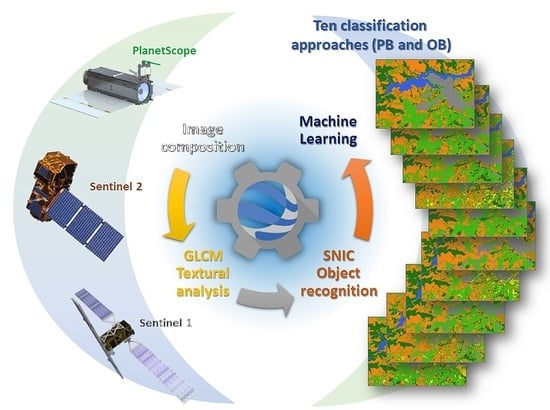
The research methodology compared ten LULC classification approaches (PB and OB, all based on the RF algorithm) applied to various dataset combinations (Table 2). In addition to five classifications of dataset combinations including PL data, five additional classifications based on S2 and S1 composite datasets were considered to extend the analysis and assess the thematic accuracy improvements of integrating PL data with S2 and S1 data. The general workflow of the research includes four main steps (Figure 2): (1) composition of the base datasets; (2) textural analysis and image segmentation; (3) LULC classification; and (4) accuracy assessment. The first step is to compose the available S2, S1, and PL images for the selected period and in the selected study area. The second is aimed at the textural analysis applying the GLCM algorithm, the image segmentation using SNIC, and the data composition to obtain the final feature dataset for the classification. The third step includes the RF classifications (PB or OB) using for training a subset of the sample points and the dataset combinations obtained in the previous steps. The last step is the accuracy assessment through a confusion matrix calculated using a validation subset of the sample points classified using the same RF classifiers of the previous step. A statistical assessment of the accuracy differences between the various classifications was performed through multiple McNemar tests.
2.3.1. Satellite Data: Sentinel-2, Sentinel-1, PlanetScope
The two European Space Agency (ESA) S2 satellites (A and B) are equipped with a multispectral sensor (MSI) that can detect 13 spectral bands with a spatial resolution of 10, 20, and 60 m and a temporal resolution of 4 days on average [48,49]. In GEE, S2 data are provided in the L1C (orthorectified top-of-atmosphere reflectance) and L2A (orthorectified atmospherically corrected surface reflectance) processing levels. Three quality assessment (QA) bands are provided at the L2A level, one of which (QA60) is a bitmask band with cloud mask information.
The S1 satellites (A and B), also launched by ESA, use a dual-polarization C-band Synthetic Aperture Radar (SAR) sensor with a spatial resolution of 10, 25, or 40 m and a temporal resolution of 6–12 days. S1 Ground Range Detected (GRD) scenes are pre-processed with the Sentinel-1 Toolbox (thermal noise removal, radiometric calibration, terrain correction) to provide the calibrated, ortho-corrected imagery available in the GEE cloud environment. Due to the S1 satellites’ operational characteristics, the S1 images are available in the study area with a revisit time of 12 days and only from descending orbits.
PlanetScope controls the world’s largest earth-observation satellite constellation, with over 150 satellites popularly known as “Doves”. These satellites have tiny dimensions (10 × 10 × 30 cm and a weight of about 4 kg) and provide daily sun-synchronous images of the entire Earth’s surface. The sensors on PL satellites capture imagery with a 3–5-m resolution and four spectral bands (RGB and NIR). PlanetScope data access from GEE is currently a paid service based on Planet’s Orders API cloud-storage destinations [50]. To access NICFI PL data, available for the tropical areas, the GEE users must follow a specific procedure and require approval by the NICFI [51]. In GEE, PL composite images are available in the WGS 84/Pseudo-Mercator (EPSG 3857) Coordinate Reference System, in contrast to the S2 and S1 images, which are georeferenced according to WGS84 (EPSG 4326).
2.3.2. Dataset Composition
Creating the base dataset is critical in the LULC classification processes [52]. In this research, the composition of the S2 dataset started by building a filtered and cloud-masked image collection of S2 L2A, including 547 images. This initial filtering was performed for the study area and the period of interest (from 1 August 2018 to 30 September 2019). The latter was defined considering the reference time of the initial ground control points dataset. Then, the Normalized Difference Vegetation Index (NDVI), the Normalized Difference Moisture Index (NDMI), the Green Normalized Difference Vegetation Index (GNDVI), and the Bare Soil Index (BSI) were calculated for each image (Table 3). The NDVI is often used to map changes in land cover [53,54] and significantly improves classification accuracy when used for the LULC classification [55]. The GNDVI and the NDMI are normalized ratios similar to the NDVI, but instead of the red band, the former uses the green band and the latter uses the short-infrared band. The GNDVI is more sensitive to the chlorophyll content of the leaves [56], whereas the NDMI is more sensitive to the water content in the spongy mesophyll of vegetation [57]. The BSI is generally used to distinguish bare soil from other land cover categories [58] and categorize and monitor seasonal bare soil locations [59]. A mean-based reduction step was applied to S2 bands and the derived spectral indices to obtain the final S2 composite dataset.
The composition of the S1 dataset was performed by initial filtering based on the same period and area of interest, instrument mode (IW), and transmitter–receiver polarizations (VV and VH). The filtered dataset includes 212 S1 images. A simple reduction was applied to obtain a final composite image containing the mean VV and VH bands. These bands were added to the S2 dataset to construct the base S2-S1 dataset.
Similarly, the PL dataset was derived by performing initial filtering based on the same period and area of interest. Considering the type of available PL images from the Planet NCFI program in the selected period, only one four-band 6-month composite image was available with a spatial resolution of 4.77 m. The NDVI and GNDVI (Table 3) were calculated from this image and added to the initial bands to obtain the base Planet composite dataset.
Before proceeding to the final band composition, to harmonize the different datasets, S2- and S1-derived layers were resampled to a resolution of 4.77 m using a bicubic interpolation [64]. The PL dataset was re-projected to the WGS84 CRS.
2.3.3. Textural Analysis and Segmentation
Object-oriented classification generally involves a segmentation stage aiming to group pixels into objects before classification. Then, on an object-by-object basis, a variety of textural, shape, and size information may be computed and used to enhance the classification and avoid the salt-and-pepper effect [56]. In this regard, we combined two steps as performed in previous studies [16,21]: the Gray-Level Co-occurrence Matrix (GLCM) for the extraction of the textural indices statistics and Simple Non-Iterative Clustering (SNIC) to identify spatial clusters (our image objects). The textural analysis and segmentation step, based on GLCM and SNIC algorithms, was applied only within the OB approaches and on the various dataset combinations used in the study (Table 2). The GLCM algorithm application in GEE computes texture metrics around each pixel of every band. The GLCM is a tabulation of how often different combinations of pixel brightness values (grey levels) occur in an image. The algorithm requires an 8-bit (gray-level) image as input. As previously undertaken in similar studies [16,21], this image was generated for S2 and PL data through a linear combination of NIR, red, and green composite bands (Equation 1). For the S1 data, after testing various indices, a normalized difference index was applied to the VV and VH bands (Equation (2)):
(0.3 × NIR) + (0.59 × RED) + (0.11 × GREEN)
(VH − VV)/(VH + VV)
The gray-level images were rescaled in the 0–255 range, using the 2nd and the 98th percentiles, before the GLCM application to improve the textural analysis results. After various tests, the window size for GLCM was set at 2 pixels for S2 and S1, and 5 pixels for PL data. Among the many textural indices calculated with GLCM, five main indices were selected for the subsequent steps (Table 4). The layers containing these textural indices, extracted from S2, S1, and PL data, were added to the other layers according to the combinations reported in Table 1 to obtain a multispectral-textural dataset.
SNIC analysis in this research was performed on the visible and NIR four bands of S2 (10 m) or PL (4.77 m) datasets. After some tests, SWIR of S2 was excluded in this step since it did not improve the image clustering process. The SNIC algorithm is an improved version of the Simple Linear Iterative Clustering (SLIC) algorithm. The algorithm clusters pixels in the combined five-dimensional color and image plane space to efficiently generate compact, nearly uniform superpixels [65]. In GEE, it identifies the objects (clusters) according to the input parameters (compactness, connectivity, neighborhood size, and seed spacing). It generates a multi-band raster including the clusters and additional layers containing the average values of the input features. Although the first three parameters were the same for S2 and PL datasets (1, 8, 128, respectively), the seed spacing was varied to account for the different native spatial resolutions and the expected average object size (S2: 8, PL: 10). These values were iteratively selected after many trials and visual analysis of SNIC outputs. The average values of the bands contained in the multispectral-textural datasets were calculated on an object basis using a “reduce connected component” step to create the dataset for the subsequent RF classification.
2.3.4. LULC Classification
The LULC classification is based on a typical supervised strategy that requires collecting the relevant information from the training points to train the classifier [66]. In GEE, a “sampleRegion” operation transfers the features’ information to the training and validation sample points. The “scale” parameter (set at 20 m for the S2 and S1 outputs, and 10 m for the PL-based outputs) averages the features locally by a downscaling step. The classification is achieved using the RF machine learning classifier, which uses bootstrap aggregation (bagging) to create multiple decision trees (DTs). The algorithm then combines the outputs using a majority voting approach to obtain a more accurate prediction. The classifiers were trained using a dataset obtained by randomly picking 70% of sample points for training, with the remaining 30% being utilized for validation. The training and validation subsets were the same for all the studied approaches to effectively compare the various approaches’ performance. In RF applications, this 70/30 ratio is quite prevalent [67,68,69]. A graph was plotted using the variable importance included in the output from the “explain” command to visualize features’ relevance in each classification. This graph was used for each approach to empirically analyze and iteratively select the more crucial bands for the LULC classification. This step increased the OB-RF classification speed and overcame some of GEE’s image size limitations.
2.3.5. Accuracy Assessment
The confusion matrix (CM) technique, a commonly used methodology based on comparing classification outputs with ground truth data, was used to assess the accuracy of the various approaches [70,71]. The matrix was used to produce specific accuracy measures: Overall Accuracy (OA, Equation (3)), Producer’s Accuracy (PA, Equation (4); also known as “recall”), and User’s Accuracy (UA, Equation (5); also known as “precision”), according to the following formulas:
The OA is commonly expressed as a percentage, with 100% accuracy indicating that all reference sites were correctly classified [72]. At the class level, PA is the ratio of true positives to the total number of true positives and false negatives, whereas UA is the ratio of true positives to the total number of true positives and false negatives. The UA is the omission error’s counterpart, whereas the PA is the commission error’s complement. The F-score is a composite measure with better sensitivity and specificity that assesses algorithm reliability [73]. It is calculated as a harmonic mean of PA and UA (Equation (6)), and it seeks to depict the balance of PA and UA [74,75] (Equation (6)). In the LULC classification, a high UA indicates a low representation of commission errors, whereas a high PA indicates a low proportion of omission errors [76].
The statistical significance of OA differences was assessed according to previous similar studies [52,77], using the McNemar test without continuity correction (with p < 0.05 as the significance threshold), which is appropriate for situations involving non-independent test datasets [78]. The kappa coefficient of agreement [79] was not calculated because the test datasets used to assess the various classification approaches were not independent [80]. Moreover, the use of kappa in assessing land cover classification accuracy has been strongly discouraged [81,82].
3. Results
The OA values obtained from the various classification approaches are compared in Table 5. The same table reports the selected features (total number, bands, and spectral and textural indices) considering their importance in each RF classification. Results of the statistical analysis of accuracy results, based on the McNemar tests, are reported in Supplementary Materials, Table S1. The only S2-derived dataset produces good accuracy from a typical RF PB method (PB_S2: 74.4%). Applying the OB approach to the same dataset, using S2-derived textures (OB_S2) substantially improves the classification obtained with the PB approach (81.6 vs. 74.4%, p = 0.005). The addition of S1 bands to the S2 dataset in the PB approach (PB_S2S1) produces a more relevant accuracy increase than PB_S2 (81.2 vs. 74.4%, p = 0.003). The OB approach on the same dataset (OB_S2S1) gives an apparent increase compared to the corresponding PB method (PB_S2S1) but is not statistically significant (83.5 vs. 81.2%, p = 0.401). Significative improvements, compared to PB_S2S1, are obtained when S1 is used for additional textural indices in the OB classification (OB_S2S1T) (86.2 vs. 81.2%, p = 0.033). Despite producing a 4.77-m resolution output, the PB method applied on only multispectral PL data (PB_PL) yields worse thematic accuracy results than the same approach applied to the S2 dataset (PB_S2) (66.7 vs. 74.4%, p = 0.014) or the S2 and S1 combined dataset (PB_S2S1) (66.7% vs. 81.2%, p = 0.000). When the OB approach is applied to the PL single-sensor dataset (OB_PL), the OA increases compared to the PB_PL (82.2 vs. 66.7%, p = 0.000). When OB_PL is compared with the same approach applied to the S2 data (OB_S2), no significant differences arise in the thematic accuracy (82.2 vs. 81.6 %, p = 0.892). Adopting the three-sensor dataset with a PB classification (PB_S2S1PL) produces a 4.77-m spatial resolution output but does not improve the OA compared to using only S2 and S1 data (PB_S2S1) (81.6 vs. 81.2%, p = 1.000). Using S2 and S1 data for the spectral information and PL data for the textural information and the object delineation in the OB method (OB_S2S1PL) noticeably increases the OA compared to the PB approach applied to the same three-sensor dataset (PB_S2S1PL) (88.3 vs. 81.6%, p = 0.002). Using the spectral bands of PL instead of those of S2 in a similar three-sensor dataset (OB_PLS2S1) apparently improves the OA compared to the previous approach (OB_S2S1PL), but the difference is not statistically significant (90.6 vs. 88.3%, p = 0.23). In contrast, the latter approaches (OB_S2S1PL and OB_PLS1S2) yield statistically significant improvements compared to the same method applied to the S2-S1 dataset (OB_S2S1) (88.3 vs. 83.5%, p = 0.004; 90.6 vs. 83.5%, p = 0.002). Unlike OB_S2S1PL, OB_PLS1S2 produces significative OA improvements compared to the OB_S2S1T, which, as indicated, includes some textural indices derived from S1 data (90.6 vs. 86.3%, p = 0.05).
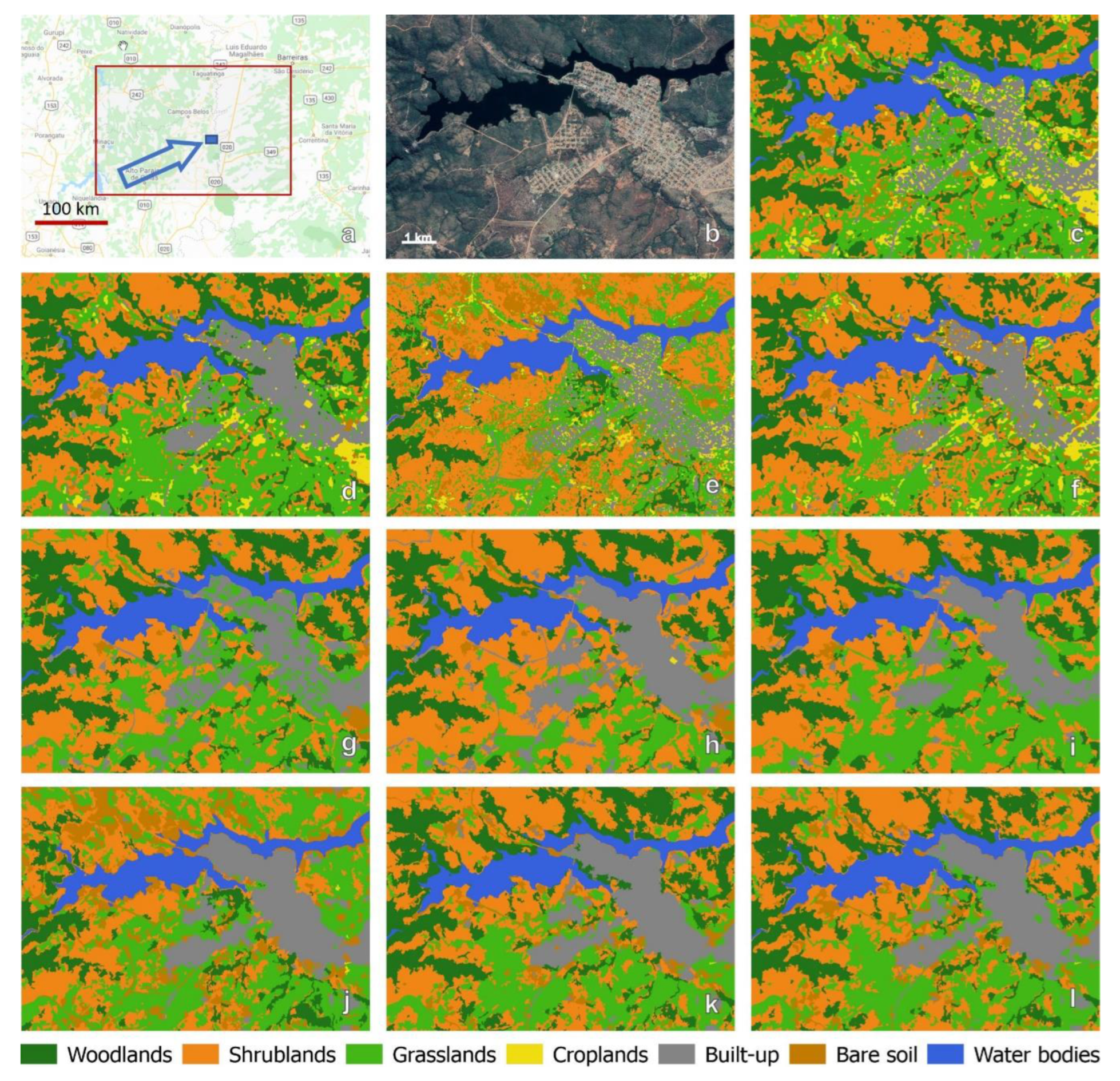
A cartographical comparison between the various classification approaches’ outputs is shown for a representative portion of the study area characterized by a built-up area, a lake portion, and a neighboring area composed of grasslands, shrublands, and scattered woodlands (Figure 3). Despite the final application of a majority filter, the output of the PB approaches suffer from the typical salt-and-pepper effect (Figure 3c–f). An evident commission between built-up areas and croplands can be detected in all the PB approaches, including that based on the three-sensor dataset. The addition of the S1 bands partially mitigates this issue (Figure 3d,f). The application of the OB approaches improves the classification results in all the studied approaches. The last two output maps, obtained from the OB procedure and the data integration of all three datasets, confirm the superior performance of these classification approaches.
Based on PA, UA, and F-scores, the analysis of accuracies at the class level shows other differences between the classification methods (Figure 4). Water bodies are omitted from the analysis considering the high accuracies obtained with all the classification approaches. According to these accuracy indices, the most problematic classes are shrublands, grasslands, bare soil, and built-up. Adding the S1 to the S2 dataset improves the classification of all the LULC classes, both in the PB (PB_S2S1) and in the OB (OB_S2S1) approaches, except the UA of woodlands. The further addition of textures derived from S1 in the OB method (OB_S2S1T) improves the UA of woodlands and grasslands, and the PA of bare soils and built-up. The OB approach to the dataset composed of S2 and S1 data (OB_S2S1) enhances the classification of croplands and built-up classes. Using only Planet data in the PB (PB_PL) and OB (OB_PL) approaches, even adding objects’ textural information in the latter, produces worse classification results, mainly for shrublands and grasslands. In addition to producing a higher-resolution LULC map, data integration of all three satellites’ data improves the classification of all LULC classes in the PB approach (PB_S2S1PL). The same integration used with the OB approaches (OB_S2S1PL and OB_PLS2S1) improves the accuracy of almost all the LULC classes, especially those most problematic for the other approaches (i.e., UA of shrublands, PA of grasslands, UA of bare soil). The slightly better performance of the OB_PLS2S1 method can be recognized mainly in UA of woodlands, PA of shrublands, and PA of grasslands.
4. Discussion
4.1. GEE and other LULC Analysis Platforms
The recent accessibility of PlanetScope data in GEE within the NICFI program offers an unprecedented high-resolution broad time series that represents a substantial advance for detecting and monitoring LULC dynamics in tropical areas. The availability of PlanetScope data in GEE, together with other various satellite imagery datasets (MODIS, Landsat, Sentinel), may offer even less-experienced GEE users an excellent opportunity to improve the detail of the land cover analysis in tropical areas. In this regard, this research contributes to assessing the potentiality of PlanetScope data for land cover classification in GEE. The initiative by NICFI runs alongside many other land cover mapping and monitoring satellite-based programs for the Amazon area, such as MAPBIOMAS [83], TerraBrasilis [84], PRODES [85], and Brazil Data Cube (BDC) [44]. At the global level, other recent global Sentinel-based mapping initiatives, such as those by ESA [86] and ESRI [87], aim to provide a homogeneous land cover map and detect and assess land cover dynamics. The approaches used in some of the programs for land cover classification of the Amazon area are often very advanced, based on object-oriented approaches and ML algorithms (such as TerraBrasilis and BDC). They provide efficient web platforms for land cover analysis and various application program interfaces (APIs) to access spatial data and algorithms.
Compared to these environments, the GEE platform appears to be more user-friendly for developing specific analyses due to the easy-to-use programming interface, the intuitive JavaScript code, the availability of advanced algorithms, the constantly growing RS imagery database, and the Map-Reduce model’s efficiency [31,84]. Furthermore, the most recent state-of-art ML algorithms can be used in GEE through the Python Google Colab environment. These features, in many cases, make GEE a preferred choice compared to traditional workstations, which are often equipped with expensive software and hardware. In this regard, GEE offers a valuable opportunity for researchers in developing countries to access a robust RS cloud-based image processing environment. However, GEE may present various drawbacks compared to other environments due to its relatively restricted programming framework. In addition, the free GEE version cannot be used for commercial uses and may not be suited for “production” workloads due to some processing, storage, and image size limits [88].
4.2. The GEE Map Composition
In the proposed methodology, the integration of the three datasets within GEE is performed during the image composition step without applying advanced data fusion techniques. In RS applications, the latter aims to improve the information contents of remotely sensed datasets used separately [89]. In this regard, in the future, advanced data fusion techniques could be incorporated into the proposed methodology to assess the possibility of further improving the accuracy of classification results. Nevertheless, considering the characteristics of the OB approach and the information enhancement obtained by the combination of its various steps, the OB method can be considered a kind of data fusion process. Furthermore, the object recognition is performed using the higher resolution images (i.e., PlanetScope), and the information coming from the lower resolution images (i.e., S2 and S1) is averaged at the object level. Thus, the OB approach can limit the effects of possible mismatching issues of images from different sensors.
The initial map composition, based on reducing several images by the period of interest (POI), is crucial in land cover classification since it allows the generation of cloud-free image composites representative of a specific time window [32,90]. In some cases, POI was widened over more years, adopting seasonal time windows in areas with frequent cloud cover when using data with relatively low temporal resolution (e.g., Landsat) [16]. This approach can generate classification inaccuracies related to the land cover changes that may occur during the POI. Thus, a compromise must be found between the need to create a cloud-free composite and limiting the effects of possible land cover changes. The POI defined for this research (14 months) is related to the time window assumed for the initial ground points dataset. The length of the POI, although it can generate the abovementioned inaccuracies, is similar to that of other studies aimed at comparing various classification approaches [21,91]. Moreover, these possible inaccuracies may equally influence the outcomes of each classification.
4.3. The Object-Based Approaches in GEE
The classification of high-resolution satellite imagery creates relevant problems related to the thematical and geometrical quality of the outputs. These issues are typically addressed using focal majority filters on the outputs of PB approaches or adopting OB classification procedures that include a preliminary step to group similar pixels. Object identification, based on advanced algorithms, is beneficial for identifying spatially continuous entities. Depending on the scale of analysis, these spatial entities may correspond from real-word objects to patches of a landscape mosaic whose textural or geometrical features are critical for their classification. In this research, in addition to measuring the improvements of the OB method on PL data, for the first time, we assessed the advantages of integrating PL imagery with Sentinel 2 and Sentinel 1 data in an OB LULC classification within GEE. Results confirmed the better performance of the OB method compared to PB methods on medium-high (S2) and high spatial resolution (PL) datasets (Table 5). The OB method, in particular, due to the textural analysis, produces a better distinction between bare soils and built-up areas, and between shrublands, croplands, and grasslands (Figure 4). The better thematic and geometrical outputs of the OB method applied to all dataset combinations become evident in the sample maps (Figure 3). This evidence was also noted in a previous, pioneer study about OB LULC classification in GEE, based on SNIC and GLCM, where three single-sensors datasets (Landsat 8, S2, and PL) were compared [21]. In this study, the OB RF classification on the single PL dataset produced worse accuracy than the S2 dataset. In contrast, in the present research, the application of an OB approach to a PL dataset, despite the lower spectral resolution, produced thematic accuracy results comparable to those obtained with the S2 dataset (Table 5), but with about double the spatial resolution. This difference is probably related to using a six-month composite instead of a single-date image. The former, resulting from a map composition performed by PlanetScope, may be more effective in the LULC classification.
4.4. Data Integration for Improving Classification Accuracy
As highlighted in previous PB LULC classifications [37,38,39], and also in this application, the integration of S1 data improved the accuracy results of the S2 dataset. This improvement is more marked in the PB approach than in the OB one. This evidence can be explained considering that the calculation of GLCM indices on S2 data provides textural information about the LULC patches that can be related to that provided by the S1 bands. The application of GLCM on S1 bands slightly improved the OB classification of the S2 and S1 composite datasets even though this improvement was statistically not significant. This evidence may appear to be in contrast with that noted in a recent study where the GLCM texture analysis on S1 images was a valuable source of information for obtaining excellent classification results of onion and sunflower in the Bonaerense Valley of the Colorado River, Argentina [92]. This difference may be related to the very different classes used in the classification. Thus, the efficacy of GLCM textural analysis on S1 data in land cover classification may strictly depend on the classes chosen for the classification and the formula used for obtaining the 8-bit grayscale image. Thus, in this regard, more investigation is necessary.
In this research, the integration of the three datasets gave the best classification results, producing a LULC map at 4.77-m resolution. As shown in the results, the integration of PL data with S2 and S1 in the PB RF classification remarkably improved the accuracy results of the only PL dataset. Similarly, the application of the OB approach on the single-sensor PL dataset produced accuracy results, also in terms of UA and PA of the various LULC classes, comparable with those obtained with the PB approach on the three-sensor dataset. This outcome confirms previous studies that focused on crop classification [42,43]. The proposed application of the OB approach to the three datasets is a further step forward considering other previous studies. The more accurate textural analysis and object identification obtained from PL data, combined with the spectral information provided by S2 and S1, enhanced the effectiveness of the three datasets’ integration. The PL bands in the visible and NIR bands (OB_PLS2S1), although not confirmed by the McNemar test, seem to perform slightly better than the correspondent S2 bands (OB_S2S1PL). This result is due mainly to a better classification of smaller features using PL higher-resolution multispectral data, as highlighted in previous studies [42,43]. In this direction, more investigation is necessary.
4.5. Possible Future Improvements
The feature selection for the RF classification was performed by identifying the potentially most-relevant textural indices and iteratively analyzing the feature importance after the classification. In similar LULC classification studies, a dimensionality reduction in textural indices was successfully performed [21,93]. However, the attempts to adopt a feature reduction step generated a block in the GEE code execution, probably due to the study area’s size. In this regard, additional experiments are required to test these approaches in OB LULC classifications based on multi-sensor datasets.
As highlighted in previous studies [16,21], all object recognition and subsequent characterization steps were developed in the raster domain, where GEE excels. However, due to the size of the study area, various export-to-asset steps were necessary to overcome the GEE image size limitations. At the same time, the selection of the most relevant spectral bands and indices, comparing the features’ importance in the RF classifications, was a significant step in reducing the classification datasets’ size. However, the proposed approach excludes consideration of object size and shape, which may be critical for objects’ classification at higher resolutions [94]. The vectorization of objects may overcome this limitation. Nonetheless, in the raster-oriented GEE environment, the few attempts we performed in this direction resulted in prolonged code execution or a processing block due to the high number of geometries.
As in similar studies, the SNIC algorithm efficiently delineated the landscape patches to be classified. Its application is usually based on a uniformly spaced grid of seeds and does not consider the local variability of objects’ size. Some attempts performed in this research to use seeds created by detecting the local minimum or maximum of variance, as suggested in previous research [16], did not produce better results. In this regard, additional research to test and develop new seeding methods will be relevant.
In addition to the thematic accuracies, it could be interesting to quantify the geometric accuracies of classifications, particularly relevant for the OBIA methods, to highlight the efficacy of the object delineation [95]. However, in addition to being particularly demanding due to the complex data acquisition, these assessment results are more suitable for OBIA on very-high-resolution data, where the landscape objects are more specifically identified [96].
5. Conclusions
To better exploit PlanetScope (PL) datasets within GEE, this work assessed the advantages of applying an object-based (OB) approach to PL data for land cover classification. Moreover, the benefits of integrating PL imagery with S2 and S1 data in a pixel-based (PB) and OB approach were evaluated. Using the PL-only dataset with a typical PB approach produced the worse overall accuracy results (67%). Adopting an OB approach on the same dataset yielded very good overall accuracy (82%), although some issues arose in classifying some classes (shrublands and bare soil). The integration of PL data with the S2 and S1 datasets improved both PB and OB accuracy outputs (82 vs. 67% and 91 vs. 82%, respectively). Although various export to asset steps were necessary, the study demonstrated the applicability of the OB approaches in GEE, even in vast study areas and on high-resolution imagery. Additional applications in other study areas, possibly including geometrical assessment and more LULC classes, may further validate the proposed approach. Including the objects’ geometrical features in the OB approach remains an open challenge in GEE.
Supplementary Materials
The following supporting information can be downloaded at: https://www.mdpi.com/article/10.3390/rs14112628/s1, Table S1: Statistical significance of the difference in OA between the ten models compared using McNemar test (significant differences with p-value < 0.05 are indicated with *).
Funding
This research received no external funding.
Data Availability Statement
Sentinel 2 and Sentinel 1 data used in the research are available within Google Earth Engine (GEE). NICFI Planet data are accessible for the tropical area within GEE after NICFI (Norway’s International Climate and Forest Initiative) approval. The GEE codes developed in this research are available by emailing the author upon any reasonable request.
Acknowledgments
The author wishes to thank Karine Reis Ferreira and Fabiana Zioti of Brazil’s National Institute for Space Research (INPE) for their valuable support for ground sample retrieval in an early stage of the research.
Conflicts of Interest
The author declares no conflict of interest.
References
- Foody, G.M. Remote sensing of tropical forest environments: Towards the monitoring of environmental resources for sustainble development. Int. J. Remote Sens. 2003, 24, 4035–4046. [Google Scholar] [CrossRef]
- Noss, R.F. Last stand: Protected areas and the defense of tropical diversity. Trends Ecol. Evol. 1997, 12, 450–451. [Google Scholar] [CrossRef]
- Shalaby, A.; Tateishi, R. Remote sensing and GIS for mapping and monitoring land cover and land-use changes in the Northwestern coastal zone of Egypt. Appl. Geogr. 2007, 27, 28–41. [Google Scholar] [CrossRef]
- Vizzari, M.; Antognelli, S.; Hilal, M.; Sigura, M.; Joly, D. Ecosystem Services Along the Urban—Rural—Natural Gradient: An Approach for a Wide Area Assessment and Mapping. In Proceedings of the Part III, Computational Science and Its Applications—ICCSA 2015: 15th International Conference, Banff, AB, Canada, 22–25 June 2015; Gervasi, O., Murgante, B., Misra, S., Gavrilova, L.M., Rocha, C.A.M.A., Torre, C., Taniar, D., Apduhan, O.B., Eds.; Springer International Publishing: Cham, Switzerland, 2015; pp. 745–757. ISBN 978-3-319-21470-2. [Google Scholar]
- Vizzari, M.; Sigura, M. Urban-rural gradient detection using multivariate spatial analysis and landscape metrics. J. Agric. Eng. 2013, 44, 453–459. [Google Scholar] [CrossRef]
- Grecchi, R.C.; Gwyn, Q.H.J.; Bénié, G.B.; Formaggio, A.R.; Fahl, F.C. Land use and land cover changes in the Brazilian Cerrado: A multidisciplinary approach to assess the impacts of agricultural expansion. Appl. Geogr. 2014, 55, 300–312. [Google Scholar] [CrossRef]
- Pelorosso, R.; Apollonio, C.; Rocchini, D.; Petroselli, A. Effects of Land Use-Land Cover Thematic Resolution on Environ-mental Evaluations. Remote Sens. 2021, 13, 1232. [Google Scholar] [CrossRef]
- Shelestov, A.; Lavreniuk, M.; Kussul, N.; Novikov, A.; Skakun, S. Exploring Google Earth Engine Platform for Big Data Processing: Classification of Multi-Temporal Satellite Imagery for Crop Mapping. Front. Earth Sci. 2017, 5, 1–10. [Google Scholar] [CrossRef] [Green Version]
- Gorelick, N.; Hancher, M.; Dixon, M.; Ilyushchenko, S.; Thau, D.; Moore, R. Remote Sensing of Environment Google Earth Engine: Planetary-scale geospatial analysis for everyone. Remote Sens. Environ. 2017, 202, 18–27. [Google Scholar] [CrossRef]
- Sullivan, B. NICFI’s Satellite Imagery of the Global Tropics Now Available in Earth Engine for Analysis|by Google Earth|Google Earth and Earth Engine|Medium. Available online: https://medium.com/google-earth/nicfis-satellite-imagery-of-the-global-tropics-now-available-in-earth-engine-for-analysis-1016df52a63d (accessed on 7 February 2022).
- NICFI Tropical Forest Basemaps Now Available in Google Earth Engine. Available online: https://www.planet.com/pulse/nicfi-tropical-forest-basemaps-now-available-in-google-earth-engine/ (accessed on 7 February 2022).
- Pfeifer, M.; Disney, M.; Quaife, T.; Marchant, R. Terrestrial ecosystems from space: A review of earth observation products for macroecology applications. Glob. Ecol. Biogeogr. 2011, 21, 603–624. [Google Scholar] [CrossRef] [Green Version]
- Mather, P.; Tso, B. Classification Methods for Remotely Sensed Data, 2nd ed.; CRC Press: Boca Raton, FL, USA, 2016; ISBN 9781420090741. [Google Scholar]
- Blaschke, T. Object based image analysis for remote sensing. ISPRS J. Photogramm. Remote Sens. 2010, 65, 2–16. [Google Scholar] [CrossRef] [Green Version]
- Torres-Sánchez, J.; López-Granados, F.; Peña, J.M. An automatic object-based method for optimal thresholding in UAV images: Application for vegetation detection in herbaceous crops. Comput. Electron. Agric. 2015, 114, 43–52. [Google Scholar] [CrossRef]
- Tassi, A.; Gigante, D.; Modica, G.; Di Martino, L.; Vizzari, M. Pixel vs. Object-Based Landsat 8 Data Classification in Google Earth Engine Using Random Forest: The Case Study of Maiella National Park. Remote Sens. 2021, 13, 2299. [Google Scholar] [CrossRef]
- Ren, X.; Malik, J. Learning a classification model for segmentation. In Proceedings of the IEEE International Conference on Computer Vision, Nice, France, 13–16 October 2003. [Google Scholar]
- Ghorbanian, A.; Kakooei, M.; Amani, M.; Mahdavi, S.; Mohammadzadeh, A.; Hasanlou, M. Improved land cover map of Iran using Sentinel imagery within Google Earth Engine and a novel automatic workflow for land cover classification using migrated training samples. ISPRS J. Photogramm. Remote Sens. 2020, 167, 276–288. [Google Scholar] [CrossRef]
- Aggarwal, N.; Srivastava, M.; Dutta, M. Comparative Analysis of Pixel-Based and Object-Based Classification of High Resolution Remote Sensing Images—A Review. Int. J. Eng. Trends Technol. 2016, 38, 5–11. [Google Scholar] [CrossRef]
- Messina, G.; Peña, J.M.; Vizzari, M.; Modica, G. A Comparison of UAV and Satellites Multispectral Imagery in Monitoring Onion Crop. An Application in the ‘Cipolla Rossa di Tropea’ (Italy). Remote Sens. 2020, 12, 3424. [Google Scholar] [CrossRef]
- Tassi, A.; Vizzari, M. Object-Oriented LULC Classification in Google Earth Engine Combining SNIC, GLCM, and Machine Learning Algorithms. Remote Sens. 2020, 12, 3776. [Google Scholar] [CrossRef]
- Hall-Beyer, M. Practical guidelines for choosing GLCM textures to use in landscape classification tasks over a range of moderate spatial scales. Int. J. Remote Sens. 2017, 38, 1312–1338. [Google Scholar] [CrossRef]
- Flanders, D.; Hall-Beyer, M.; Pereverzoff, J. Preliminary evaluation of eCognition object-based software for cut block de-lineation and feature extraction. Can. J. Remote Sens. 2003, 29, 441–452. [Google Scholar] [CrossRef]
- Singh, M.; Evans, D.; Friess, D.A.; Tan, B.S.; Nin, C.S. Mapping Above-Ground Biomass in a Tropical Forest in Cambodia Using Canopy Textures Derived from Google Earth. Remote Sens. 2015, 7, 5057–5076. [Google Scholar] [CrossRef] [Green Version]
- Li, M.; Zhang, R.; Luo, H.; Gu, S.; Qin, Z. Crop Mapping in the Sanjiang Plain Using an Improved Object-Oriented Method Based on Google Earth Engine and Combined Growth Period Attributes. Remote Sens. 2022, 14, 273. [Google Scholar] [CrossRef]
- Loukika, K.N.; Keesara, V.R.; Sridhar, V. Analysis of Land Use and Land Cover Using Machine Learning Algorithms on Google Earth Engine for Munneru River Basin, India. Sustainability 2021, 13, 13758. [Google Scholar] [CrossRef]
- Luo, C.; Qi, B.; Liu, H.; Guo, D.; Lu, L.; Fu, Q.; Shao, Y. Using Time Series Sentinel-1 Images for Object-Oriented Crop Classification in Google Earth Engine. Remote Sens. 2021, 13, 561. [Google Scholar] [CrossRef]
- Breiman, L. Random forests. Mach. Learn. 2001, 45, 5–32. [Google Scholar] [CrossRef] [Green Version]
- Gislason, P.O.; Benediktsson, J.A.; Sveinsson, J.R. Random forests for land cover classification. Pattern Recognit. Lett. 2006, 27, 294–300. [Google Scholar] [CrossRef]
- Mountrakis, G.; Im, J.; Ogole, C. Support vector machines in remote sensing: A review. ISPRS J. Photogramm. Remote Sens. 2011, 66, 247–259. [Google Scholar] [CrossRef]
- Amani, M.; Ghorbanian, A.; Ahmadi, S.A.; Kakooei, M.; Moghimi, A.; Mirmazloumi, S.M.; Moghaddam, S.H.A.; Mahdavi, S.; Ghahremanloo, M.; Parsian, S.; et al. Google Earth Engine Cloud Computing Platform for Remote Sensing Big Data Applications: A Comprehensive Review. IEEE J. Sel. Top. Appl. Earth Obs. Remote Sens. 2020, 13, 5326–5350. [Google Scholar] [CrossRef]
- Praticò, S.; Solano, F.; Di Fazio, S.; Modica, G. Machine Learning Classification of Mediterranean Forest Habitats in Google Earth Engine Based on Seasonal Sentinel-2 Time-Series and Input Image Composition Optimisation. Remote Sens. 2021, 13, 586. [Google Scholar] [CrossRef]
- Nery, T.; Sadler, R.; Solis-Aulestia, M.; White, B.; Polyakov, M.; Chalak, M. Comparing supervised algorithms in Land Use and Land Cover classification of a Landsat time-series. In Proceedings of the International Geoscience and Remote Sensing Symposium (IGARSS), Beijing, China, 10–15 July 2016. [Google Scholar]
- Rodriguez-Galiano, V.F.; Ghimire, B.; Rogan, J.; Chica-Olmo, M.; Rigol-Sanchez, J.P. An assessment of the effectiveness of a random forest classifier for land-cover classification. ISPRS J. Photogramm. Remote Sens. 2012, 67, 93–104. [Google Scholar] [CrossRef]
- Costa, J. da S.; Liesenberg, V.; Schimalski, M.B.; de Sousa, R.V.; Biffi, L.J.; Gomes, A.R.; Neto, S.L.R.; Mitishita, E.; Bispo, P. da C. Benefits of Combining ALOS/PALSAR-2 and Sentinel-2A Data in the Classification of Land Cover Classes in the Santa Catarina Southern Plateau. Remote Sens. 2021, 13, 229. [Google Scholar] [CrossRef]
- Mizuochi, H.; Iijima, Y.; Nagano, H.; Kotani, A.; Hiyama, T. Dynamic Mapping of Subarctic Surface Water by Fusion of Microwave and Optical Satellite Data Using Conditional Adversarial Networks. Remote Sens. 2021, 13, 175. [Google Scholar] [CrossRef]
- De Luca, G.; Silva, J.M.N.; Di Fazio, S.; Modica, G. Integrated use of Sentinel-1 and Sentinel-2 data and open-source machine learning algorithms for land cover mapping in a Mediterranean region. Eur. J. Remote Sens. 2022, 55, 52–70. [Google Scholar] [CrossRef]
- Tavus, B.; Kocaman, S.; Gokceoglu, C. Flood damage assessment with Sentinel-1 and Sentinel-2 data after Sardoba dam break with GLCM features and Random Forest method. Sci. Total Environ. 2022, 816, 151585. [Google Scholar] [CrossRef]
- Tavares, P.A.; Beltrão, N.E.S.; Guimarães, U.S.; Teodoro, A.C. Integration of Sentinel-1 and Sentinel-2 for Classification and LULC Mapping in the Urban Area of Belém, Eastern Brazilian Amazon. Sensors 2019, 19, 1140. [Google Scholar] [CrossRef] [Green Version]
- Carrasco, L.; O’Neil, A.W.; Daniel Morton, R.; Rowland, C.S. Evaluating Combinations of Temporally Aggregated Sentinel-1, Sentinel-2 and Landsat 8 for Land Cover Mapping with Google Earth Engine. Remote Sens. 2019, 11, 288. [Google Scholar] [CrossRef] [Green Version]
- Javhar, A.; Chen, X.; Bao, A.; Jamshed, A.; Yunus, M.; Jovid, A.; Latipa, T. Comparison of Multi-Resolution Optical Land-sat-8, Sentinel-2 and Radar Sentinel-1 Data for Automatic Lineament Extraction: A Case Study of Alichur Area, SE Pamir. Remote Sens. 2019, 11, 778. [Google Scholar] [CrossRef] [Green Version]
- Rao, P.; Zhou, W.; Bhattarai, N.; Srivastava, A.K.; Singh, B.; Poonia, S.; Lobell, D.B.; Jain, M. Using Sentinel-1, Sentinel-2, and Planet Imagery to Map Crop Type of Smallholder Farms. Remote Sens. 2021, 13, 1870. [Google Scholar] [CrossRef]
- Kpienbaareh, D.; Sun, X.; Wang, J.; Luginaah, I.; Kerr, R.B.; Lupafya, E.; Dakishoni, L. Crop Type and Land Cover Mapping in Northern Malawi Using the Integration of Sentinel-1, Sentinel-2, and PlanetScope Satellite Data. Remote Sens. 2021, 13, 700. [Google Scholar] [CrossRef]
- Brazil Data Cube—Plataforma para Análise e Visualização de Grandes Volumes de Dados Geoespaciais. Available online: http://brazildatacube.org/en/home-page-2/ (accessed on 25 March 2022).
- Carta della Natura—Italiano. Available online: https://www.isprambiente.gov.it/it/servizi/sistema-carta-della-natura (accessed on 25 March 2021).
- Hansen, M.C.; Roy, D.P.; Lindquist, E.; Adusei, B.; Justice, C.O.; Altstatt, A. A method for integrating MODIS and Landsat data for systematic monitoring of forest cover and change in the Congo Basin. Remote Sens. Environ. 2008, 112, 2495–2513. [Google Scholar] [CrossRef]
- Llano, X.C. SMByC-IDEAM. AcATaMa—QGIS Plugin for Accuracy Assessment of Thematic Maps. Available online: https://github.com/SMByC/AcATaMa (accessed on 27 May 2022).
- ESA. User Guides—Sentinel-2—Sentinel Online. Available online: https://sentinel.esa.int/web/sentinel/user-guides/sentinel-2-msi/overview (accessed on 12 October 2020).
- Santaga, F.S.; Agnelli, A.; Leccese, A.; Vizzari, M. Using Sentinel-2 for Simplifying Soil Sampling and Mapping: Two Case Studies in Umbria, Italy. Remote Sens. 2021, 13, 3379. [Google Scholar] [CrossRef]
- Planet GEE Delivery Overview. Available online: https://developers.planet.com/docs/integrations/gee/ (accessed on 8 February 2022).
- Use NICFI—Planet Lab Data—SEPAL Documentation. Available online: https://docs.sepal.io/en/latest/setup/nicfi.html (accessed on 8 February 2022).
- Phan, T.N.; Kuch, V.; Lehnert, L.W. Land Cover Classification using Google Earth Engine and Random Forest Classifier—The Role of Image Composition. Remote Sens. 2020, 12, 2411. [Google Scholar] [CrossRef]
- Lunetta, R.S.; Knight, J.F.; Ediriwickrema, J.; Lyon, J.G.; Worthy, L.D. Land-cover change detection using multi-temporal MODIS NDVI data. Remote Sens. Environ. 2006, 105, 142–154. [Google Scholar] [CrossRef]
- Woodcock, C.E.; Macomber, S.A.; Kumar, L. Vegetation mapping and monitoring. In Environmental Modelling with GIS and Remote Sensing; Taylor & Francis: London, UK, 2010. [Google Scholar]
- Singh, R.P.; Singh, N.; Singh, S.; Mukherjee, S. Normalized Difference Vegetation Index (NDVI) Based Classification to Assess the Change in Land Use/Land Cover (LULC) in Lower Assam, India. Int. J. Adv. Remote Sens. GIS 2016, 5, 1963–1970. [Google Scholar] [CrossRef]
- Moges, S.M.; Raun, W.R.; Mullen, R.W.; Freeman, K.W.; Johnson, G.V.; Solie, J.B. Evaluation of green, red, and near infrared bands for predicting winter wheat biomass, nitrogen uptake, and final grain yield. J. Plant Nutr. 2004, 27, 1431–1441. [Google Scholar] [CrossRef]
- Yang, X.; Zhao, S.; Qin, X.; Zhao, N.; Liang, L. Mapping of urban surface water bodies from sentinel-2 MSI imagery at 10 m resolution via NDWI-based image sharpening. Remote Sens. 2017, 9, 596. [Google Scholar] [CrossRef] [Green Version]
- Diek, S.; Fornallaz, F.; Schaepman, M.E.; de Jong, R. Barest Pixel Composite for agricultural areas using landsat time series. Remote Sens. 2017, 9, 1245. [Google Scholar] [CrossRef] [Green Version]
- Chen, W.; Liu, L.; Zhang, C.; Wang, J.; Wang, J.; Pan, Y. Monitoring the seasonal bare soil areas in Beijing using multi-temporal TM images. In Proceedings of the International Geoscience and Remote Sensing Symposium (IGARSS), Anchorage, AK, USA, 20–24 September 2004. [Google Scholar]
- Rouse, J.W., Jr.; Haas, R.H.; Schell, J.A.; Deering, D.W. Monitoring vegetation systems in the great plains with erts. In Proceedings of the 3rd ERTS-1 Symposium (NASA SP-351), Washington, DC, USA, 10–14 December 1973; pp. 309–317. [Google Scholar]
- Gitelson, A.A.; Kaufman, Y.J.; Merzlyak, M.N. Use of a green channel in remote sensing of global vegetation from EOS-MODIS. Remote Sens. Environ. 1996, 58, 289–298. [Google Scholar] [CrossRef]
- Hardisky, M.A.; Klemas, V.; Smart, R.M. The influence of soil salinity, growth form, and leaf moisture on the spectral ra-diance of Spartina alterniflora canopies. Photogramm. Eng. Remote Sens. 1983, 49, 77–83. [Google Scholar]
- Rikimaru, A.; Roy, P.S.; Miyatake, S. Tropical forest cover density mapping. Trop. Ecol. 2002, 43, 39–47. [Google Scholar]
- Keys, R.G. Cubic Convolution Interpolation for Digital Image Processing. IEEE Trans. Acoust. 1981, 29, 1153–1160. [Google Scholar] [CrossRef] [Green Version]
- Achanta, R.; Süsstrunk, S. Superpixels and polygons using simple non-iterative clustering. In Proceedings of the 30th IEEE Conference on Computer Vision and Pattern Recognition, CVPR 2017, Honolulu, HI, USA, 21–26 July 2017. [Google Scholar]
- Chen, D.M.; Stow, D. The effect of training strategies on supervised classification at different spatial resolutions. Photogramm. Eng. Remote Sens. 2002, 68, 1155–1161. [Google Scholar]
- Mueller, J.P.; Massaron, L. Training, Validating, and Testing in Machine Learning. Available online: https://www.dummies.com/programming/big-data/data-science/training-validating-testing-machine-learning/ (accessed on 7 June 2021).
- Adelabu, S.; Mutanga, O.; Adam, E. Testing the reliability and stability of the internal accuracy assessment of random forest for classifying tree defoliation levels using different validation methods. Geocarto Int. 2015, 30, 810–821. [Google Scholar] [CrossRef]
- Chen, W.; Xie, X.; Wang, J.; Pradhan, B.; Hong, H.; Bui, D.T.; Duan, Z.; Ma, J. A comparative study of logistic model tree, random forest, and classification and regression tree models for spatial prediction of landslide susceptibility. Catena 2017, 151, 147–160. [Google Scholar] [CrossRef] [Green Version]
- Congalton, R.G. A review of assessing the accuracy of classifications of remotely sensed data. Remote Sens. Environ. 1991, 37, 35–46. [Google Scholar] [CrossRef]
- Liu, C.; Frazier, P.; Kumar, L. Comparative assessment of the measures of thematic classification accuracy. Remote Sens. Environ. 2007, 107, 606–616. [Google Scholar] [CrossRef]
- Al-Saady, Y.; Merkel, B.; Al-Tawash, B.; Al-Suhail, Q. Land use and land cover (LULC) mapping and change detection in the Little Zab River Basin (LZRB), Kurdistan Region, NE Iraq and NW Iran. FOG—Freib. Online Geosci. 2015, 43, 1–32. [Google Scholar]
- Sokolova, M.; Japkowicz, N.; Szpakowicz, S. Beyond accuracy, F-score and ROC: A family of discriminant measures for performance evaluation. In Proceedings of the AAAI Workshop; Technical Report; AAAI Press: Palo Alto, CA, USA, 2006. [Google Scholar]
- Taubenböck, H.; Esch, T.; Felbier, A.; Roth, A.; Dech, S. Pattern-based accuracy assessment of an urban footprint classifi-cation using TerraSAR-X data. IEEE Geosci. Remote Sens. Lett. 2011, 8, 278–282. [Google Scholar] [CrossRef]
- Stehman, S.V. Statistical rigor and practical utility in thematic map accuracy assessment. Photogramm. Eng. Remote Sens. 2001, 67, 727–734. [Google Scholar]
- Weaver, J.; Moore, B.; Reith, A.; McKee, J.; Lunga, D. A comparison of machine learning techniques to extract human set-tlements from high resolution imagery. In Proceedings of the International Geoscience and Remote Sensing Symposium (IGARSS), Valencia, Spain, 22–27 July 2018. [Google Scholar]
- Hurskainen, P.; Adhikari, H.; Siljander, M.; Pellikka, P.K.E.; Hemp, A. Auxiliary datasets improve accuracy of object-based land use/land cover classification in heterogeneous savanna landscapes. Remote Sens. Environ. 2019, 233, 111354. [Google Scholar] [CrossRef]
- Foody, G.M. Thematic map comparison: Evaluating the statistical significance of differences in classification accuracy. Photogramm. Eng. Remote Sens. 2004, 70, 627–633. [Google Scholar] [CrossRef]
- Lunetta, R.S.; Congalton, R.G.; Fenstermaker, L.K.; Jensen, J.R.; McGwire, K.C.; Tinney, L.R. Remote sensing and geographic information system data integration: Error sources and research issues. Photogramm. Eng. Remote Sens. 1991, 57, 677–687. [Google Scholar]
- Foody, G.M.; Mathur, A. A relative evaluation of multiclass image classification by support vector machines. IEEE Trans. Geosci. Remote Sens. 2004, 42, 1335–1343. [Google Scholar] [CrossRef] [Green Version]
- Foody, G.M. Explaining the unsuitability of the kappa coefficient in the assessment and comparison of the accuracy of thematic maps obtained by image classification. Remote Sens. Environ. 2020, 239, 111630. [Google Scholar] [CrossRef]
- Olofsson, P.; Foody, G.M.; Herold, M.; Stehman, S.V.; Woodcock, C.E.; Wulder, M.A. Good practices for estimating area and assessing accuracy of land change. Remote Sens. Environ. 2014, 148, 42–57. [Google Scholar] [CrossRef]
- Mapbiomas Brasil. Available online: https://mapbiomas.org/en (accessed on 29 April 2022).
- Fernando, L.; Assis, F.G.; Ferreira, K.R.; Vinhas, L.; Maurano, L.; Almeida, C.; Carvalho, A.; Rodrigues, J.; Maciel, A.; Ca-margo, C. TerraBrasilis: A Spatial Data Analytics Infrastructure for Large-Scale Thematic Mapping. ISPRS Int. J. Geo-Inf. 2019, 8, 513. [Google Scholar] [CrossRef] [Green Version]
- PRODES—Coordenação-Geral de Observação da Terra. Available online: http://www.obt.inpe.br/OBT/assuntos/programas/amazonia/prodes (accessed on 29 April 2022).
- European Space Agency WorldCover. Available online: https://esa-worldcover.org/en (accessed on 27 May 2022).
- Karra, K.; Kontgis, C.; Statman-Weil, Z.; Mazzariello, J.C.; Mathis, M.; Brumby, S.P. Global land use/land cover with Sentinel 2 and deep learning. In Proceedings of the International Geoscience and Remote Sensing Symposium (IGARSS), Brussels, Belgium, 11–16 July 2021; Volume 2021. [Google Scholar]
- Maas, M.D. 5 Things to Consider about Google Earth Engine. Available online: https://www.matecdev.com/posts/disadvantages-earth-engine.html (accessed on 29 April 2022).
- Chang, N.B.; Bai, K. Multisensor Data Fusion and Machine Learning for Environmental Remote Sensing; CRC Press: Boca Raton, FL, USA, 2018. [Google Scholar]
- Thanh Noi, P.; Kappas, M. Comparison of Random Forest, k-Nearest Neighbor, and Support Vector Machine Classifiers for Land Cover Classification Using Sentinel-2 Imagery. Sensors 2018, 18, 18. [Google Scholar] [CrossRef] [Green Version]
- Yang, Y.; Yang, D.; Wang, X.; Zhang, Z.; Nawaz, Z. Testing accuracy of land cover classification algorithms in the qilian mountains based on gee cloud platform. Remote Sens. 2021, 13, 5064. [Google Scholar] [CrossRef]
- Caballero, G.R.; Platzeck, G.; Pezzola, A.; Casella, A.; Winschel, C.; Silva, S.S.; Ludueña, E.; Pasqualotto, N.; Delegido, J. Assessment of Multi-Date Sentinel-1 Polarizations and GLCM Texture Features Capacity for Onion and Sunflower Classification in an Irrigated Valley: An Object Level Approach. Agronomy 2020, 10, 845. [Google Scholar] [CrossRef]
- Stromann, O.; Nascetti, A.; Yousif, O.; Ban, Y. Dimensionality Reduction and Feature Selection for Object-Based Land Cover Classification based on Sentinel-1 and Sentinel-2 Time Series Using Google Earth Engine. Remote Sens. 2020, 12, 76. [Google Scholar] [CrossRef] [Green Version]
- Mathieu, R.; Aryal, J.; Chong, A.K. Object-Based Classification of Ikonos Imagery for Mapping Large-Scale Vegetation Communities in Urban Areas. Sensors 2007, 7, 2860–2880. [Google Scholar] [CrossRef] [Green Version]
- Cai, L.; Shi, W.; Miao, Z.; Hao, M. Accuracy Assessment Measures for Object Extraction from Remote Sensing Images. Remote Sens. 2018, 10, 303. [Google Scholar] [CrossRef] [Green Version]
- Radoux, J.; Bogaert, P.; Kerle, N.; Gerke, M.; Lefèvre, S.; Gloaguen, R.; Thenkabail, P.S. Good Practices for Object-Based Accuracy Assessment. Remote Sens. 2017, 9, 646. [Google Scholar] [CrossRef] [Green Version]
Figure 1.
Study area location in Brazil (a,b). Visible and infra-red composite images of PlanetScope (c,d) and Sentinel 2 (e,f). VV (g) and VH (h) composite images of Sentinel 1.
Figure 1.
Study area location in Brazil (a,b). Visible and infra-red composite images of PlanetScope (c,d) and Sentinel 2 (e,f). VV (g) and VH (h) composite images of Sentinel 1.

Figure 2.
The methodological workflow of the research.

Figure 3.
Comparison of LULC classification approaches in a representative region of the study area. Location of the area (blue arrow and rectangle) within the study area (red rectangle) (a), Google aerial view (b), 1_PB_S2 (c), 2_PB_S2S1 (d), 3_PB_PL (e), 4_PB_S2S1PL (f), 5_OB_S2 (g), 6_OB_S2S1 (h), 7_OB_S2S1T (i), 8_OB_PL (j), 9_OB_S2S1PL (k), 10_OB_PLS2S1 (l). Codes are reported in Table 2.

Figure 4.
Comparison of user’s (a) and producer’s (b) accuracies, and F-scores (c) of the classification approaches (Y axis) obtained for the various LULC classes (X axis). Water bodies are omitted. Codes used in the legend for classification approaches are reported in Table 2.
Figure 4.
Comparison of user’s (a) and producer’s (b) accuracies, and F-scores (c) of the classification approaches (Y axis) obtained for the various LULC classes (X axis). Water bodies are omitted. Codes used in the legend for classification approaches are reported in Table 2.


Table 1.
Land cover classes and number of sample points used in the research.
| Land Cover Classes | Number of Sample Points |
|---|---|
| Woodlands | 341 |
| Shrublands | 457 |
| Grasslands | 424 |
| Croplands | 422 |
| Built-up | 225 |
| Bare soil | 286 |
| Water bodies | 245 |
Table 2.
Sources of multispectral and textural information and datasets used for object recognition in the various approaches compared in the research. PB: pixel-based, OB: object-based, S2: Sentinel 2, S1: Sentinel 1, PL: PlanetScope.
Table 2.
Sources of multispectral and textural information and datasets used for object recognition in the various approaches compared in the research. PB: pixel-based, OB: object-based, S2: Sentinel 2, S1: Sentinel 1, PL: PlanetScope.
| Approach Type | Approach Code | Multispectral Information | Textural Information | Object Recognition |
|---|---|---|---|---|
| PB | PB_S2 | S2 | - | - |
| PB_S2S1 | S2, S1 | - | - | |
| PB_PL | PL | - | - | |
| PB_S2S1PL | S2, S1, PL | - | - | |
| OB | OB_S2 | S2 | S2 | S2 |
| OB_S2S1 | S2, S1 | S2 | S2 | |
| OB_S2S1T | S2, S1 | S2, S1 | S2 | |
| OB_PL | PL | PL | PL | |
| OB_S2S1PL | S2, S1 | PL | PL | |
| OB_PLS2S1 | PL, S2, S1 | PL | PL |
Table 3.
Spectral indices and related formulas used in the research.
| Index | Formula | Author |
|---|---|---|
| NDVI | Rouse et al., 1973 [60] | |
| GNDVI | Gitelson et al., 1996 [61] | |
| NDMI | Hardisky et al., 1983 [62] | |
| BSI | Rikimaru et al., 2002 [63] |
Table 4.
Textural indices calculated using the Gray-Level Co-occurrence Matrix (GLCM).
| CODE | Textural Index Description |
|---|---|
| ASM | Angular Second Moment: measures the number of repeated pairs in the image |
| CONTR | Contrast: measures the local contrast of an image |
| CORR | Correlation: measures the correlation between pairs of pixels in the image |
| VAR | Variance: measures how spread out the distribution of gray-levels is in the image |
| IDM | Inverse Difference Moment: measures the homogeneity of the image |
Table 5.
LULC classification approaches, number of features, bands, and indices selected for the classification, output resolution, and overall accuracy (OA). Classification approaches’ codes are reported in Table 2. S2 features are in upper case, S1 features are in italic upper case, and PlanetScope features are in lower case. Spectral indices (NDVI, GNDVI, NDMI, BSI) are reported in Table 3. Textural index codes and descriptions are reported in Table 4. The statistical significance of the OA differences between the classifications is shown in Table S1.
| CODE | Number of Selected Features | Selected Spectral Bands and Indices | Textural Indices | Output Resolution (m) | OA |
|---|---|---|---|---|---|
| PB_S2 | 9 | B2, B4, B8, B11, B12, NDVI, GNDVI, NDMI, BSI | - | 10 | 0.744 |
| PB_S2S1 | 11 | B2, B4, B8, B11, B12, NDVI, GNDVI, NDMI, BSI, VV, VH | - | 10 | 0.812 |
| PB_PL | 6 | b, g, r, n, NDVI, GNDVI | - | 4.77 | 0.667 |
| PB_S2S1PL | 12 | b, g, r, n, B11, B12, NDVI, GNDVI, NDMI, BSI, VV, VH | - | 4.77 | 0.816 |
| OB_S2 | 14 | B2, B4, B8, B11, B12, NDVI, GNDVI, NDMI, BSI | ASM, CONTR, CORR, VAR, IDM | 10 | 0.816 |
| OB_S2S1 | 16 | B2, B4, B8, B11, B12, NDVI, GNDVI, NDMI, BSI, VV, VH | ASM, CONTR, CORR, VAR, IDM | 10 | 0.835 |
| OB_S2S1T | 19 | B2, B4, B8, B11, B12, NDVI, GNDVI, NDMI, BSI, VV, VH | ASM, CONTR, CORR, VAR, IDM, ASM, CONTR, IDM | 10 | 0.863 |
| OB_PL | 11 | b, g, r, n, ndvi, gndvi | asm, contr, corr, var, idm | 4.77 | 0.822 |
| OB_S2S1PL | 16 | B2, B4, B8, B11, B12, NDVI, GNDVI, NDMI, BSI, VV, VH | asm, contr, corr, var, idm | 4.77 | 0.883 |
| OB_PLS2S1 | 16 | b, r, n, B11, B12, NDVI, GNDVI, NDMI, BSI, VV, VH | asm, contr, corr, var, idm | 4.77 | 0.906 |
Publisher’s Note: MDPI stays neutral with regard to jurisdictional claims in published maps and institutional affiliations. |
© 2022 by the author. Licensee MDPI, Basel, Switzerland. This article is an open access article distributed under the terms and conditions of the Creative Commons Attribution (CC BY) license (https://creativecommons.org/licenses/by/4.0/).
Share and Cite
MDPI and ACS Style
Vizzari, M. PlanetScope, Sentinel-2, and Sentinel-1 Data Integration for Object-Based Land Cover Classification in Google Earth Engine. Remote Sens. 2022, 14, 2628. https://doi.org/10.3390/rs14112628
AMA Style
Vizzari M. PlanetScope, Sentinel-2, and Sentinel-1 Data Integration for Object-Based Land Cover Classification in Google Earth Engine. Remote Sensing. 2022; 14(11):2628. https://doi.org/10.3390/rs14112628
Chicago/Turabian StyleVizzari, Marco. 2022. "PlanetScope, Sentinel-2, and Sentinel-1 Data Integration for Object-Based Land Cover Classification in Google Earth Engine" Remote Sensing 14, no. 11: 2628. https://doi.org/10.3390/rs14112628
Note that from the first issue of 2016, this journal uses article numbers instead of page numbers. See further details here.