
Land Surface Snow Phenology Based on an Improved Downscaling Method in the Southern Gansu Plateau, China


Key Laboratory of Western China’s Environmental Systems (Ministry of Education), College of Earth and Environmental Sciences, Lanzhou University, No. 222 South Tianshui Road, Chengguan District, Lanzhou 730000, China
*
Author to whom correspondence should be addressed.
Remote Sens. 2022, 14(12), 2848; https://doi.org/10.3390/rs14122848
Submission received: 17 May 2022
/
Revised: 8 June 2022
/
Accepted: 11 June 2022
/
Published: 14 June 2022
(This article belongs to the Special Issue Land-Atmosphere Interactions and Effects on the Climate of the Tibetan Plateau and Surrounding Regions)
Abstract
:Snow is involved in and influences water–energy processes at multiple scales. Studies on land surface snow phenology are an important part of cryosphere science and are a hot spot in the hydrological community. In this study, we improved a statistical downscaling method by introducing a spatial probability distribution function to obtain regional snow depth data with higher spatial resolution. Based on this, the southern Gansu Plateau (SGP), an important water source region in the upper reaches of the Yellow River, was taken as a study area to quantify regional land surface snow phenology variation, together with a discussion of their responses to land surface terrain and local climate, during the period from 2003 to 2018. The results revealed that the improved downscaling method was satisfactory for snow depth data reprocessing according to comparisons with gauge-based data. The downscaled snow depth data were used to conduct spatial analysis and it was found that snow depth was on average larger and maintained longer in areas with higher altitudes, varying and decreasing with a shortened persistence time. Snow was also found more on steeper terrain, although it was indistinguishable among various aspects. The former is mostly located at high altitudes in the SGP, where lower temperatures and higher precipitation provide favorable conditions for snow accumulation. Climatically, factors such as precipitation, solar radiation, and air temperature had significantly singular effectiveness on land surface snow phenology. Precipitation was positively correlated with snow accumulation and maintenance, while solar radiation and air temperature functioned negatively. Comparatively, the quantity of snow was more sensitive to solar radiation, while its persistence was more sensitive to air temperature, especially extremely low temperatures. This study presents an example of data and methods to analyze regional land surface snow phenology dynamics, and the results may provide references for better understanding water formation, distribution, and evolution in alpine water source areas.
1. Introduction
Snow is one of the main forms of water in the cryosphere and is involved in most land surface energy and moisture transport [1,2,3]. It influences local and regional land–atmospheric processes and circulation [4,5] and is considered an important indicator of environmental changes at multiple scales [6,7]. Variations in snow and its phenology directly affect the formation of mountain discharge and the evolution of water resources in river source areas [8,9], influencing water utilization and supporting local society–economy–ecological sustainability in the middle and lower reaches [10,11]. Quantitative analysis can help better understand the responses of land surface hydrological systems to environmental changes [12,13,14].
Snow is very sensitive to climate change. According to the 6th Assessment Report of the Intergovernmental Panel on Climate Change (IPCC), the current global air temperature is approximately 1 °C higher than before industrialization. In terms of the predicted average temperature change in the next 20 years, the global temperature rise is expected to reach or exceed 1.5 °C [15,16]. Future warming may lead to abnormal precipitation and accelerated and earlier glacier and snow melts, which, in turn, will affect the distribution and dynamics of snow in time and space [17,18]. Studies have revealed that the spatiotemporal distribution of snow cover shows strong differentiation in China, and relatively stable snow areas are found mainly in northwestern and northeastern China, the Tibetan Plateau, and Inner Mongolia [19,20,21]. Land surface snow phenology (LSSP), such as snow cover start date, snow melt end date, and snow depth, is better correlated with temperature than other meteorological factors.
Underlying conditions, such as land surface topography and vegetation types, also affect the distribution and dynamics of snow [22,23]. For example, as the temperature gradually decreases with increasing altitude, snow melt slows, making it easier for snow to accumulate [24,25]. The absorption of solar radiation changes with different terrain conditions (i.e., slope and aspect), leading to diverse environmental temperatures and heating, consequentially influencing snowmelt processes [26,27]. In addition, relatively open areas, such as forest edges and sparse woodlands, are prone to snow accumulation, and the opposite is the case in well-covered woodlands due to canopy interception [28,29,30].
In recent decades, an increasing number of programs have been initiated internationally to facilitate snow research, such as the Climate and Cryosphere Project of the World Climate Research Program (WCRP), the Cold Region Land Surface Processes Experiment carried out by NASA, and the Western Environmental and Ecological Science Research Project, effectively advancing not only the study of snow and its dynamics as the key objects [31,32,33], but also techniques for snow monitoring and data derivation. In particular, the idea of using optical remote sensing to obtain snow information has made great progress [34,35,36], a large number of derivations as data products have been released, such as microwave radiometer-based (i.e., AMSR-E) and MODIS-based (i.e., MOD10A1 and MOD10A2) [37,38,39]. Among them, MODIS-based snow products have high spatial resolutions, can better reflect the distribution of snow cover, and are widely used in regional snow variation-related studies [40,41,42]. In contrast, passive microwave monitoring-based snow depth data are useful for equivalent evaluation, but their spatial resolution is generally low [43,44,45]. To obtain high-resolution snow depth information, downscaling of the data is needed. There are two common methods for this purpose: one is based on statistics, and the other is based on deep learning such as machine training [41,46]. The development of downscaling methods is important for snow studies, especially when conducted at smaller scales [47,48,49].
The southern Gansu Plateau (SGP), located on the northeast edge of the Tibetan Plateau, is an important water source area in the upper reaches of China’s Yellow River and Yangtze River. Snow dynamics effectively influence runoff formation and evolution, and mechanistic exploration is beneficial to the scientific planning and utilization of basin water resources [5,50]. Over the past 20 years, river discharge on the SGP have sharply decreased, although few studies on snow phenology and its hydro effectiveness have been published. In view of the above, the objectives of this study are (1) to improve a downscaling method to obtain high-resolution snow depth (SD) data for the analysis of spatiotemporal variations in LSSP on the SGP during the time period from 2003–2018 and (2) to use a geostatistical method to analyze the effects of topographic and climatic factors on the LSSP. Related results may help improve our knowledge of alpine-cold region snow and can provide basic data and methodological support for comprehensive hydrological simulations and predictions in the water source area of large river basins.
2. Study Area
As an important part of the water source area in the upper reaches of the Yellow River, the SGP administratively includes the whole of the Gannan Tibetan Autonomous Prefecture in Gansu Province of China, geographically located between 33°06′N–35°34′N, 100°45′E–104°45′E (Figure 1a). The elevation ranges from 1159~4866 m and averages approximately 3000 m, topographically featuring higher elevations in the northwest and lower elevations in the southeast. The regionally averaged annual air temperature is 1.7 °C, featuring a short frost-free period and plentiful sunshine throughout the year. The annual total precipitation is 620 mm, concentrated in the rainy season from June to September. The relatively lower air temperature and abundant precipitation, corresponding to a typically continental plateau climate, make the SGP naturally develop many tributary systems of the Yellow River (i.e., the Tao River, the Daxia River, etc.) and Yangtze River (i.e., the Bailong River), becoming remarkable in terms of water conservation on the Tibetan Plateau (Figure 1b,c). Along with the increasing intensity of human activities such as cultivation and overgrazing, ecosystems such as grasslands and wetlands become ecologically fragile, and water yield recharge to rivers are reduced, both seriously affecting the protection of regional water resources and ecological security. Due to the significance of snowmelt to SGP hydro-processes, the analysis of snow distribution and dynamics is important for the formation, evolution, rational development, and utilization of water on the SGP and across all the related basins.
3. Data and Methods
3.1. Data
The SD data were obtained from the long-term series of the daily snow depth dataset in China (1979–2020), released by the National Tibetan Plateau data center (http://data.tpdc.ac.cn, accessed on 11 October 2021). The data were derived from the inversion of daily passive microwave brightness temperature (SMMR, SSM/I, and SSMI/S), with a spatial resolution of 0.25° [51]. Based on the daily SD data, the monthly and annual maximum SD data were obtained using the maximum value composite (MVC) method, which represented the maximum value in the process of snowmelt and accumulation [52]. The snow cover data were adopted from the MODIS Daily Cloudless 500 m Snow Area Product Dataset over China during the period from 2000 to 2019, released by the National Cryosphere Desert Data Center (http://www.ncdc.ac.cn, accessed on 28 October 2021), used for LSSP calculation [53]. A DEM with a 30 m spatial resolution released by the Chinese Academy of Sciences Geospatial Data Cloud (http://www.gscloud.cn, accessed on 5 July 2018) was used to calculate the slope and aspect across the SGP. The surface net solar radiation data were released by the European Centre for Medium-Range Weather Forecasts (ECMWF) (https://www.ecmwf.int/, accessed on 17 April 2019), with a spatial resolution of 0.25° and a temporal resolution of 3 h. The meteorological data, including precipitation, maximum temperature, and minimum temperature, were from the National Meteorological Information Center of China Meteorological Administration (http://data.cma.cn/, accessed on 21 August 2021). Snow depth observation data came from the National Meteorological Information Center of the China Meteorological Administration and are used to test the accuracy of the downscaling. The time spans of the above data (except for the DEM) were unified to the same period from 2002 to 2018 for simultaneity.
3.2. Methods
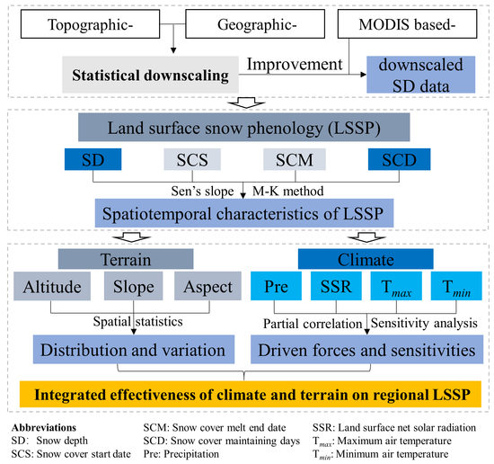
3.2.1. SD Data Downscaling
We define the spatial resolution of 0.25° as the lower resolution and that of 500 m as the finer resolution. The purpose of this is to downscale the lower resolution SD data to the finer resolution by considering and integrating multiple influential factors.
(1) Statistical downscaling
Pilot correlation analysis revealed that topographic and geographic factors such as elevation, slope, aspect, longitude, and latitude have significant effects on SD; they affect or regulate climatic process such as snowfall at local or even larger scales [54,55]. All the above factors were calculated and resampled into the lower and finer spatial resolutions. Taking the influential factors at coarse resolution as environmental variables, a multiple linear regression method is used to calibrate the statistical formula based on the original monthly 0.25° SD data () as the target variable. Application of the formula results in a simulated series of SD at both the lower (, Equation (1)) and finer (, Equation (3)) spatial resolutions. Residuals (Equation (2)) of to () are resampled into the finer 500 m resolution () using bilinear interpolation. The sums of and are the statistically downscaled SD data (, Equation (4)).
where (n = 1, 2, 3, 4, 5) represent raster data of elevation, slope, aspect, longitude, and latitude, respectively. Subscripts low and high denote the lower and finer resolutions in space, respectively.
(2) Improvement based on snow cover data
The original resolution of the SD data is 0.25°, and although it has been geographically and topographically corrected through statistical downscaling, the inaccurate influence is still present. For example, SD occurs in low-altitude regions in warmer months, a situation that seldom occurs, as common sense in the study area dictates. By introducing the spatial distribution probability function of snow, the 500 m MODIS snow cover data are used to modify and improve the precision of the statistical downscaling. Given values of 1 and 0 representing snowy and snowless pixels, respectively, the original MODIS snow cover raster data are converted into binary ones. We define the period from September 1 of one year to August 31 of the next year as a snow hydrological year (SHY), and the accumulation days of snow (ADS) in each SHY are calculated from September 2002 to August 2018 at a spatial resolution of 500 m. Then, the cumulative days of snow (CDS) in a domain containing 55 × 55 ADS grids are counted, approximately corresponding to the spatial resolution of the original SD data (). The snow distribution probability () can be determined as follows:
The product of and (Equation (6)) is what objective (1) aims at, which is an improvement of the statistically downscaled SD based on snow cover data, comprehensively reflecting a high-resolution SD () controlled or influenced by geography, topography, and snow distribution (Figure 2).
3.2.2. LSSP Indicator Extraction
Snow cover maintaining days (SCD), snow cover start date (SCS), and snow cover melt end date (SCM) are calculated based on the binary retreated MODIS snow cover data. Among them, SCS and SCM are important LSSPs determining SCD [56,57], which represent the dates when a monitored pixel starts accumulating snow and ends melting in a SHY. SCD is the number of days that each pixel is covered by snow in a SHY. The larger the SCD is, the longer and the more the snow reserves.
In the above equations, is a fixed number representing the date when the largest snow cover occurs during the period from 2002 to 2018. The statistics resulted in the date being 12 January 2008, the 134th day in the SHY. and represent the numbers of snow cover days before and after , respectively, in each SHY. N is the upper limit for a specified time range, valued as 1 to represent a complete SHY; is the binary retreated pixel value of daily snow cover (snowy or snowless).
3.2.3. Trend Analysis
Sen’s slope is selected for series variation amplitude statistics [58,59]. The method can reduce or prevent the impact of data anomalies and omissions when evaluating the trend and range of time series changes. An orderly column is constructed with the change rates of sample sequences of different lengths. Variable testing is then performed statistically according to the given significance level to obtain the value range of the change rates, and the median is used to determine the variation trend and magnitude. The equation is as follows:
where is Sen’s slope, and represent the sequential values corresponding to time and , respectively, where 1 < < < n and n is the length of the series.
The Mann–Kendall method [60,61] is a nonparametric test approach used to determine the significance of a trend analysis [62].
where and represent the snow phenology indicators in SHY and , respectively; n represents the length of the sequence. A positive value of the statistic S indicates an increasing trend of the data series, while a negative one indicates a decreasing trend of the series. The value of Z is in the range of (−∞, +∞); for a given confidence interval α, if |Z| ≥ , it indicates that there is a significant trend in the data series at confidence level α.
3.2.4. Analysis of Climate-Driven Influences
Correlation-based significance statistics, represented by partial correlation coefficients, are used to examine the strength of climate influences on regional LSSP. To be specific, assuming there are ( > 2) variables (, ......, , , ), the formula for the th order partial correlation coefficient of any two variables and is:
where r denotes the correlation coefficient, factors on the right side of the formula are the ()th order partial factors.
Four key climatic factors, including precipitation (P), land surface net solar radiation (SSR), maximum air temperature (Tmax), and minimum air temperature (Tmin), are selected to investigate the climate-driven strength of the LSSP, the 3rd order partial correlation coefficient is adopted. A t test is used to analyze whether the partial correlation coefficient between LSSP and climatic factors pass the 0.01 significance level (Table 1). The calculation formula is:
where is the partial correlation coefficient, m is the number of independent variables, and n is the sequence length. The partitioning criteria are listed in Table 1.
3.2.5. Sensitivity Analysis
The response of snow variation to climate change is diagnosed using the sensitivity coefficient [63]. The method is widely used in contribution separations of influential factors on hydrological processes. The sensitivity coefficient is calculated as:
where is the sensitivity coefficient of (LSSP) to (climatic factors), indicating that the % change in LSSP is caused by 1% variation in a climatic element. and are the multiyear averaged values of and . In the following statement, represents the sensitivity of LSSP to climatic factors, a is climatic factors such as P, SSR, Tmax, and Tmin, b is LSSP indicators such as SD and SCD.
4. Results
4.1. Evaluation of the Improved SD Downscaling Method
Gauge-based SD observations at 10 stations in and near the SGP (Figure 1c) were adopted as references, based on which absolute errors were calculated using SD data before and after downscaling, as shown in Figure 3. The vertical ranges cover all errors, including both the positive and negative ones, while transverse widths indicate occurrent frequencies. It can be seen that the positive downscaled SD () errors at all stations and the negative errors at most of the 10 stations are reduced, indicating an effective optimization for the elimination of both the over- and underestimations of the initial SD data. Frequencies of SD error valued at 0 were found to be the highest at all stations, and differences were not clear between the two sets of data, although an overall but slight decrease appeared. As a whole, using the improved downscaling method, the spatial resolution and real representation of SD were verified to be acceptable, and the downscaled data were satisfactory for LSSP analysis in the SGP region.
4.2. LSSP Characteristics
The binary retreated MODIS snow cover data were used to calculate time-based LSSP values, including the SCS, SCM, and SCD. Together with the downscaled SD data, a spatiotemporal analysis of LSSPs of the SGP from 2002 to 2018 was conducted.
4.2.1. Spatiotemporal Distributions
LSSPs present remarkable heterogeneity in time and space on the SGP. High SD values are mainly found in areas near or at mountain divides, while low SD values are generally distributed in valley areas featuring lower altitudes. For example, in the southwestern and southeastern parts where the main stream of the Yellow River and the Bailong River develop, SD can exceed 18 cm in high altitude zones but less than 10 cm in valleys (Figure 4a). The SCS and SCM show opposite distribution patterns in value space (Figure 4b,c). In or near mountain divides, snow begins to accumulate early (i.e., the earliest is the 34th day in a SHY) but ends melting late (i.e., after the 255th day in a SHY). In most areas, the SCS starts after the 120th day, corresponding to SCM days before the 195th day, and both result in a relatively short SCD time in a SHY, i.e., most of the SCD is quantified to be less than 15 days in the SGP. Overall, the SD, SCS, SCM, and SCD spatially match well in phenology. For example, in areas such as mountain divides featuring deeper snow, accumulation starts earlier, melting ends later, and snow cover lasts longer.
The SD is larger in months from November to the following March than that in the rest of a SHY, the maximum value generally occurs in February, with a multiyear average value of 4.03 cm (Figure 5a). For the presence of snow cover, SCD presents a “multipeak” pattern in a SHY (Figure 5b). Generally, snow cover lasts the longest in November of one year and March of the following year, especially in March, when the existence of snow can reach 8 days. In the context of the regional climate, there is rarely snow cover in the SGP from June to August.
4.2.2. Spatiotemporal Variations
LSSP variation was found to interannually fluctuate according to quantification of the representative index, including SD, SCS, SCM, and SCD. Generally, higher values of SD and SCD occurred simultaneously, corresponding to smaller SCS values and larger SCM values (Figure 6). During the period from 2003 to 2018, the value ranges of the LSSP index, such as the SD, SCS, SCM, and SCD, were quantified from 2.67 to 10.53 cm, 113 to 134 d, 142 to 188 d, and 16 to 75 d, averaged to 5.15 cm, 123 d, 158 d, and 34 d, respectively. During the statistical period, the maximum SD was found in 2009, when the SCS and SCM were 121 d and 181 d in the SHY, respectively, corresponding to an SCD length of 60 d.
The variation trends and amplitudes of the LSSP during the time period from 2003 to 2018 were measured spatially on the SGP based on Sen’s slope method, as shown in Figure 7. A decreasing trend of SD in most of the area occurred, especially in the southwestern part, which is located in the main channel of the Yellow River. A relatively small area had an increase in SD, as in the southeastern part, which dominates the upstream section of the Bailong River. The variation in SD was not significant at p ≥ 0.01 on most of the SGP, especially in the central and northern parts, similar to the significance test for the spatial statistics of the other three LSSP indices. The areal percentage of the reduced SD occupied 60.36%, and the variation amplitude was overall quantified into a rate of −0.06 cm/a across the whole SGP (Figure 7a). Areas with high altitudes showed significant changes in the SCS and SCM, such as in or near mountain divides. In terms of the areal percentage, areas with increased SCS accounted for 75.10%, indicating that the start date of snow accumulation on most of the SGP presented a delay. Areas with decreased SCM accounted for 65.78%, indicating that most of the snow melt ended earlier. However, the aggregative variation was rated as 0.53 d/a and 0.45 d/a for SCS and SCM, respectively (Figure 7b,c). The amplitude of the former was greater than that of the latter, resulting in an overall reduction in SCD of −0.37 d/a, which was specifically significant in the southwestern and southeastern parts of the SGP. The statistics resulted in a larger areal percentage of 56.90% for the increase in SCD, and the overall reduction was due to the magnitude of the decrease (Figure 7d).
4.3. Terrain Influence on LSSP
Terrain factors, including altitude, slope, and aspect, were calculated and reclassified using value intervals of 500 m, 10°, and 45° for analysis of the topographic influence on the LSSP. Altitude zones between 3000~3500 m and 3500~4000 m are mostly distributed in the region (Figure 8a), while few of the slopes are more than 50° (Figure 8b). The aspect differentiation is not significant, with relatively more differentiation in the northeast and less differentiation in the southeast and south (Figure 8c).
4.3.1. Terrain-Based Distribution
LSSP presented a similar value distribution corresponding to altitude and slope. Statistically, the higher the altitude, or the steeper the slope, the greater the SD (Figure 9a,c), SCM (Figure 9c,f) and SCD (Figure 9d,h), and the smaller the SCS (Figure 9b,g). In particular, the variation amplitudes of the four LSSP indices increased along with the above two terrain factors, indicating that LSSP variability strengthened in regions with higher altitudes and steeper slopes. Generally, snow does not easily accumulate on steep slopes, our analysis showed an inverse pattern. It was found that steep slopes are mostly located in regions with high altitudes on the SGP and are more prone to snowfall, which might be the reason why the higher SD values were more distributed [64]. The influence of aspects on LSSP were statistically close due to the relative equilibrium at the regional scale. South-facing areas, including the southeast, south, and southwest facings, had smaller SD, SCM, and SCD, and larger SCS (Figure 9i–l), reflecting a lower probability of snow accumulation on sunny slopes.
4.3.2. Terrain-Based Variation
Statistics were conducted to diagnose the variation difference in the LSSP corresponding to the reclassified terrain. The results revealed that the decrease in SD mainly occurred in regions with altitudes higher than 3000 m, while in other altitude zones, the SD increased. In zones with slopes ranging between 70~80° or less than 40°, the SD was found to decrease, although an increase occurred in other slope zones. All aspects, correspondingly exhibiting almost all altitudes and slopes in zones, were found to decrease with SD. In terms of the time phenology, an increase in SCS, together with a decrease in SCM, was found in most of the altitude zones, resulting in a general decrease in SCD or a shortened snow-maintaining time, especially in regions with altitudes higher than 3000 m, consistent with the variation in SD (Figure 10a). The SCS in all slope zones presented a delay (increase), while the SCM presented a decrease (earlier), except in zones with slopes less than 20° (Figure 10b). Statistics based on aspects resulted in an overall increase in the SCS and SCM, although the variation rates of the latter were less than those of the former (Figure 10c). According to the above, given an altitude of 3000 m and a slope of 20°, LSSPs on the SGP generally presented a pattern of “decrease in higher and steeper areas corresponding to a shortened snow duration, increase in lower and flatter areas corresponding to a relatively lengthened snow duration”, which might have a profound relationship with the regional climate change under the warming background.
4.4. Climate Influence on LSSP
Analysis revealed that the SGP experienced an overall reduction in snow accumulation during the time period from 2003 to 2018, the duration of snow cover moved backward in a SHY. The above, represented by the SD and SCD indices (determined by SCS and SCM), can be considered comprehensive reflections of snow dynamics. Reasons leading to snow variation vary, in which the climate influence plays an important role [25,65]. In particular, regional precipitation (P), surface net solar radiation (SSR), maximum air temperature (Tmax), and minimum air temperature (Tmin) are key factors [66] and are thus selected to analyze the responses of the LSSP to regional climate change on the SGP.
4.4.1. Partial Correlation Analysis
The influence of climate change on regional LSSP is mechanically complex. To be more focused, the multicollinearity analysis between factors of climate and terrain are ignored at this stage because it is out of the present study’s scope. Given the four selected climatic factors, the singular or synergistic effectiveness of multiple factor combinations on LSSP variation needs to be clarified. Coupling partial correlation (Equation (14)) and significance analysis (Table 1) can help. Among the 16 factor/combinations, the top five categories satisfying the t test standard were sorted by significantly influenced area. The SD order list was [SSR, Tmin, Tmax, SSR + Tmin, P] (Figure 11a), while that of the SCD was [Tmax, SSR, P, P + SSR + Tmax, P + Tmax] (Figure 11b), indicating different impacts of climate on regional LSSP variation, e.g., SD varied remarkably by SSR and Tmin effectiveness, although SCD was more susceptible to synergistic influences, mechanically showing more complexity. Effectiveness of climatic driving factors on SD and SCD were found to be different, which may be due to local terrain regulations to different LSSP. For example, in the northern part of the SGP featuring lower altitude, the SD is more significantly related to lower air temperature that facilitating more snowfall, while the occurrence of factors with influence that can significantly drive the SCD is less because snow is usually sparse and shortly maintained there. In the southwestern part, the altitude is relatively higher and the air temperature is always lower; the abundant SSR, due to the high altitude, influences SD more, although SCD is dramatically affected by the higher air temperature because the snow event occurs commonly, especially in cold seasons. In summary, the singular effectiveness of the factors was verified to influence the LSSP more over a larger area, which may be related to the zonal differentiation of terrain and climate on the SGP. In other words, key factors affecting regional LSSP might tend to be single, which is in good agreement with the following sensitivity analysis.
4.4.2. Sensitivity Analysis
Sensitivity (coefficient) analysis quantifies the percentage variation in the target variable (SD/SCD) caused by a 1% change in the environmental variable (the climatic factors). , , and represent the sensitivity of SD to P, SSR, Tmax, and Tmin, respectively. The results revealed that SD positively or negatively responded to all four climatic factors. Positive facilitation of SD due to increased P was widely characterized on the SGP, accounting for 67.74% of the area (Figure 12a), while the other three factors produced damping effects on SD; along with the increase in SD, the proportions of the area with negative impacts were above 80% (Figure 12b–d). The regional averages of , , and were 0.71%, −4.12%, −3.22%, and −2.95%, respectively, corresponding to SD variation rates when the climatic factor increased by 1%. Comparatively, SD was more sensitive to SSR on the SGP.
, , , and represent the sensitivity of SCD to P, SSR, Tmax, and Tmin, respectively. Similar results were obtained by calculations (Figure 13). In contrast, the regional averages of , , , and were 1.16%, −3.69%, −3.45%, and −4.01%, respectively, corresponding to SCD variation rates when the climatic factor increased by 1%. Comparatively, SCD was more sensitive to air temperature, especially the lower ones.
Overall, the LSSP on the SGP was influenced by and showed more sensitivity to solar radiation and air temperature. Local precipitation, especially snowfall, provides the matter base for snow formation, distribution, and accumulation. The low sensitivity might be related to the spatiotemporal correspondence and the interactive adaptation between terrain and climate.
4.5. Integrated Effectiveness of Climate and Terrain
To explore the integrated effectiveness of climate and terrain, statistics of LSSP sensitivity (coefficients) to the climate were conducted based on the terrain. The results showed negative values of with respect to the area, mainly at altitudes lower than 3000 m, while positive values were observed in the others, indicating that precipitation tended to positively contribute to SD in higher altitude regions [67]. Values of were found to be positive in most of the study area except in the altitude range of 1500~2000 m, indicating that it is not easy for snow to form and be maintained in lower altitude regions. The sensitivity coefficients of the two LSSP indices to SSR, Tmax, and Tmin were all negative, indicating that an increase in the three climate factors led to a decrease in snow in both amount and persistence at all altitudes (Figure 14a,b). In areas with slopes greater than 30°, the SD sensitivity to precipitation was found to be negative, indicating that snow hardly accumulated on steep slopes. The SCD sensitivity to precipitation was positive but decreased with increasing slope, indicating that the steeper the slope is, the smaller the effect of precipitation on snow persistence. The absolute value of LSSP sensitivity to SSR and Tmax decreased with increasing slope, while the trend of LSSP sensitivity to Tmin was opposite, meaning that snow on steeper land is less sensitive to solar radiation and higher air temperature, but more sensitive to lower air temperature (Figure 14c,d). LSSP sensitivities to P and SSR were not found to be significantly different in various aspects, while LSSP sensitivity to Tmax was found to be stronger on sunny (southward) slopes and LSSP sensitivity to Tmin was stronger on shaded (northward) slopes (Figure 14e,f).
5. Discussion
Located in a midlatitude inland region featuring limitations of circulation transportation, precipitation, especially snowfall in the cold season on the SGP, is relatively scarce [41]. Combined with the influence of land surface topography, snow cover presents remarkable fragmentation [68,69], leading to significant heterogeneity in LSSP variation [70]. For a better understanding, data with a fine spatial resolution are thus essential. To address this issue, we regressively analyzed the relationship between SD and the geographic and topographic factors on the SGP to statistically downscale the SD data product from a coarse spatial resolution of 0.25° to a finer one of 500 m. To eliminate the distortion of the original data, we introduced the MODIS-based spatial probability of snow cover for correction [7,71]. The coupling of the two ideas not only helped advance the downscaling method but also improved the data accuracy of snow depth, which can be considered an example to synthesize methods in data treatment.
Snow formation, accumulation, and redistribution are closely related to land surface terrain [72,73]. We found that on the SGP, the higher the altitude is, the larger the LSSP variability, indicating that snow is more significantly affected by environmental factors at higher altitudes [74]. The slope, together with aspect, is profoundly connected with incidence angle and eolian activities, acting on the amount of solar radiation and energy flux, influencing land surface energy budget, and affecting snow accumulation and melt rates [68,75]. Our study demonstrated the difference in LSSP in terrains with high complexity.
It was found that precipitation and air temperature are the key factors that most influence the regional LSSP [76]. As the basic material source for forming snow, precipitation cannot have an effect on the LSSP unless the air temperature is below the freezing point [77,78], which might be the explanation for the lower sensitivity of the LSSP to precipitation and the more remarkable sensitivity to air temperature [79,80]. Generally, absorption of solar radiation by snow cover relates to land surface albedo [81,82], during which the phase variation of the solar altitude angle in winter and spring plays an important role, dramatically affecting snow melt in a year [83,84]. Our study of the SGP agree with the above findings. The influence of key climatic factors on LSSP was further distinguished, and considerable differences in LSSP in response to the maximum and minimum air temperatures in time and space were quantitatively presented.
In terms of LSSP variation, the chemical composition and physical state of the atmosphere (e.g., aerosol load), structure and density of snow (e.g., crystal size) [85], variation in environmental conditions (e.g., permafrost degradation [82]; land use/cover change [86]), artificial disturbance [87,88], and so on, directly or indirectly have profound impact on snow accumulation and melting and may cause LSSP variability [89]. In particular, a long period with snow is generally influenced by combinations of interactively functioning factors [90]. Our study examined individual effectiveness based on sensitivity analysis, and coupling studies were not conducted. Additionally, LSSP does not vary synchronously with climate, and delays with time often occur [78,91]. Furthermore, land surface vegetation also influences the LSSP [92]. The above processes, together with their effects on regional LSSP, have been neglected and may lead to uncertainties in the present study. It is hoped that shortcomings will be overcome in the future based on the improvement of data and methods.
6. Conclusions
In this study, we developed an improved statistical downscaling method to obtain SD data with higher spatial resolution for a comprehensive study on regional LSSP of the SGP, a specifically selected water source area of China’s Yellow River. It was shown that the improved downscaling method can be used to effectively optimize both the spatial resolution and data accuracy of SD. Statistics from 2003 to 2018 revealed an overall reduction in the SGP’s LSSP, especially the two main indices of SD and SCD, which varied at negative rates of −0.06 cm/a and −0.37 d/a, respectively. In terms of terrain, the LSSP of the SGP generally presented a pattern of “decrease in higher and steeper areas corresponding to a shortened snow duration, increase in lower and flatter areas corresponding to a relatively lengthened duration”. Climatically, given a 1% increase in P, SSR, Tmax and Tmin, the regional averages of the SD variation were 0.71%, −4.12%, −3.22%, and −2.95%, respectively, while those of the SCD variation were 1.16%, −3.69%, −3.45%, and −4.01%, respectively. Comparatively, SD was more sensitive to SSR, while SCD was more sensitive to air temperature on the SGP. These findings may be helpful to the awareness of snow hydrology and promote its quantitative analysis in the alpine water source areas of large river basins.
Author Contributions
L.W.: data collection, methodology, writing—original draft. C.L.: supervision, formal analysis, conceptualization, writing—review and editing. X.X.: data analysis. S.Z., J.L., X.Z. and N.S.: writing—review and editing. All authors have read and agreed to the published version of the manuscript.
Funding
This study was supported by the Key Research Programs of Gansu Province in Science and Technology (20ZD7FA005, 21ZD4FA008), the Open Foundation of MOE Key Laboratory of Western China’s Environmental System in Lanzhou University as the Fundamental Research Funds for the Central Universities (lzujbky-2020-kb01).
Data Availability Statement
The long-term series of the daily snow depth dataset in China are available in the National Tibetan Plateau data center. These data were derived from the flowing resources available in the public domain: http://data.tpdc.ac.cn. The MODIS Daily Cloudless 500 m Snow Area Product Dataset over China are available in the National Cryosphere Desert Data Center. These data were derived from the flowing resources available in the public domain: http://www.ncdc.ac.cn. The surface net solar radiation data were released by the European Centre for Medium-Range Weather Forecasts (ECMWF) (https://www.ecmwf.int/). The meteorological data were from the National Meteorological Information Center of China Meteorological Administration (http://data.cma.cn/ all accessed on 7 June 2022).
Acknowledgments
We are grateful to the National Meteorological Science Data Center, National Tibetan Plateau Data Center, National Cryosphere Desert Data Center, NASA, and the ECMWF for providing open access to data collections and archives.
Conflicts of Interest
The authors declare that they have no conflict of interest.
Abbreviations
| LSSP | Land surface snow phenology |
| SGP | Southern Gansu Plateau |
| SD | Snow depth |
| MVC | Maximum value composite |
| ECMWF | European Centre for Medium-Range Weather Forecasts |
| SHY | Snow hydrological year |
| CDS | Cumulative days of snow |
| ADS | Accumulation days of snow |
| SCD | Snow cover maintaining days |
| SCS | Snow cover start date |
| SCM | Snow cover melt end date |
| Tmax | Maximum air temperature |
| Tmin | Minimum air temperature |
| SSR | Land surface net solar radiation |
References
- Yi, Y.; Liu, S.; Zhu, Y.; Wu, K.; Xie, F.; Saifullah, M. Spatiotemporal heterogeneity of snow cover in the central and western Karakoram Mountains based on a refined MODIS product during 2002–2018. Atmos. Res. 2020, 250, 105402. [Google Scholar] [CrossRef]
- Zhong, X.; Zhang, T.; Kang, S.; Wang, J. Spatiotemporal variability of snow cover timing and duration over the Eurasian continent during 1966–2012. Sci. Total Environ. 2021, 750, 141670. [Google Scholar] [CrossRef] [PubMed]
- Erickson, T.A.; Williams, M.W.; Winstral, A. Persistence of topographic controls on the spatial distribution of snow in rugged mountain terrain, Colorado, United States. Water. Resour. Res. 2005, 41, W04014. [Google Scholar] [CrossRef] [Green Version]
- Bavay, M.; Grunewald, T.; Lehning, M. Response of snow cover and runoff to climate change in high Alpine catchments of Eastern Switzerland. Adv. Water Resour. 2013, 55, 4–16. [Google Scholar] [CrossRef]
- Chen, H.; Chen, Y.; Li, W.; Li, Z. Quantifying the contributions of snow/glacier meltwater to river runoff in the Tianshan Mountains, Central Asia. Global Planet. Chang. 2019, 174, 47–57. [Google Scholar] [CrossRef]
- Tarca, G.; Guglielmin, M.; Convey, P.; Worland, W.R.; Cannone, N. Small-scale spatial–temporal variability in snow cover and relationships with vegetation and climate in maritime Antarctica. Catena 2021, 208, 105739. [Google Scholar] [CrossRef]
- Xie, J.; Jonas, T.; Rixen, C.; Jong, R.; Garonna, I.; Notarnicola, C.; Asam, S.; Schaepman, M.E.; Kneubuhler, M. Land surface phenology and greenness in Alpine grasslands driven by seasonal snow and meteorological factors. Sci. Total Environ. 2020, 725, 138380. [Google Scholar] [CrossRef]
- Thornton, J.; Brauchli, T.; Mariethoz, G.; Brunner, P. Efficient multi-objective calibration and uncertainty analysis of distributed snow simulations in rugged alpine terrain. J. Hydrol. 2021, 598, 126241. [Google Scholar] [CrossRef]
- Lehning, M.; Lowe, H.; Ryser, M.; Raderschall, N. Inhomogeneous precipitation distribution and snow transport in steep terrain. Water Resour. Res. 2008, 44, W07404. [Google Scholar]
- Thapa, S.; Zhang, F.; Zhang, H.; Zeng, C.; Wang, L.; Xu, C.; Thapa, A.; Nepal, S. Assessing the snow cover dynamics and its relationship with different hydro-climatic characteristics in Upper Ganges river basin and its sub-basins. Sci. Total Environ. 2021, 793, 148648. [Google Scholar] [CrossRef]
- Wu, X.; Wang, X.; Liu, S.; Yang, Y.; Xu, G.; Xu, Y.; Jiang, T.; Xiao, C. Snow cover loss compounding the future economic vulnerability of western China. Sci. Total Environ. 2021, 755, 143025. [Google Scholar] [CrossRef] [PubMed]
- Juras, R.; Blocher, J.; Jenicek, M.; Hotovy, O.; Markonis, Y. What affects the hydrological response of rain-on-snow events in low-altitude mountain ranges in Central Europe? J. Hydrol. 2021, 603, 127002. [Google Scholar] [CrossRef]
- Zhang, H.; Immerzeel, W.; Zhang, F.; Kok, R.; Chen, D.; Yan, W. Snow cover persistence reverses the altitudinal patterns of warming above and below 5000 m on the Tibetan Plateau. Sci. Total Environ. 2021, 803, 149889. [Google Scholar] [CrossRef] [PubMed]
- Nepal, S.; Khatiwada, K.; Pradhananga, S.; Kralisch, S.; Samyn, D.; Bromand, M.T.; Jamal, N.; Dildar, M.; Durrani, F.; Rassouly, F.; et al. Future snow projections in a small basin of the Western Himalaya. Sci. Total Environ. 2021, 795, 148587. [Google Scholar] [CrossRef]
- IPCC. Climate Change 2021: The Physical Science Basis. Contribution of Working Group I to the Sixth Assessment Report of the Intergovernmental Panel on Climate Change; Cambridge University Press: London, UK, 2021; in press. [Google Scholar]
- Ishtiaque, A.; Estoque, R.; Eakin, H.; Parajuli, J.; Rabby, Y. IPCC’s current conceptualization of ‘vulnerability’ needs more clarification for climate change vulnerability assessments. J. Environ. Manag. 2022, 303, 114246. [Google Scholar] [CrossRef] [PubMed]
- Zhong, X.; Zhang, T.; Su, H.; Xiao, X.; Wang, S.; Hu, Y.; Wang, H.; Zheng, L.; Zhang, W.; Xu, M.; et al. Impacts of landscape and climatic factors on snow cover in the Altai Mountains, China. Adv. Clim. Chang. Res. 2021, 12, 95–107. [Google Scholar] [CrossRef]
- Collados-Lara, A.; Pardo-Iguzquiza, E.; Pulido- Veelazquez, D. A distributed cellular automata model to simulate potential future impacts of climate change on snow cover area. Adv. Water Resour. 2019, 124, 106–119. [Google Scholar] [CrossRef]
- Yang, W.; Jin, F.; Si, Y.; Li, Z. Runoff change controlled by combined effects of multiple environmental factors in a headwater catchment with cold and arid climate in northwest China. Sci. Total Environ. 2021, 756, 143995. [Google Scholar] [CrossRef]
- Hao, Y.; Sun, F.; Wang, H.; Liu, W.; Shen, Y.; Li, Z.; Hu, S. Understanding climate-induced changes of snow hydrological processes in the Kaidu River Basin through the CemaNeige-GR6J model. Catena 2022, 212, 106082. [Google Scholar] [CrossRef]
- Sun, S.; Kang, S.; Guo, J.; Zhang, Q.; Paudyal, R.; Sun, X.; Qin, D. Insights into mercury in glacier snow and its incorporation into meltwater runoff based on observations in the southern Tibetan Plateau. J. Environ. Sci. 2018, 68, 130–142. [Google Scholar] [CrossRef]
- Smith, T.; Rheinwalt, A.; Bookhagen, B. Topography and climate in the upper Indus Basin: Mapping elevation-snow cover relationships. Sci. Total Environ. 2021, 786, 147363. [Google Scholar] [CrossRef] [PubMed]
- Saydi, M.; Ding, J. Impacts of topographic factors on regional snow cover characteristics. Water Sci. Eng. 2020, 13, 171–180. [Google Scholar] [CrossRef]
- Lehning, M.; Grunewald, T.; Schirmer, M. Mountain snow distribution governed by an altitudinal gradient and terrain roughness. Geophys. Res. Lett. 2011, 38, L19504. [Google Scholar] [CrossRef] [Green Version]
- Tang, G.; Li, S.; Yang, M.; Xu, Z.; Liu, Y.; Gu, H. Streamflow response to snow regime shift associated with climate variability in four mountain watersheds in the US Great Basin. J. Hydrol. 2019, 573, 255–266. [Google Scholar] [CrossRef]
- Zwaaftink, C.; Mott, R.; Lehning, M. Seasonal simulation of drifting snow sublimation in Alpine terrain. Water Resour. Res. 2013, 49, 1581–1590. [Google Scholar] [CrossRef] [Green Version]
- Helbig, N.; Herwijnen, A. Subgrid parameterization for snow depth over mountainous terrain from flat field snow depth. Water Resour. Res. 2017, 53, 1444–1456. [Google Scholar] [CrossRef] [Green Version]
- Zaremehrjardy, M.; Razzavi, S.; Faramarzi, M. Assessment of the cascade of uncertainty in future snow depth projections across watersheds of mountainous, foothill, and plain areas in northern latitudes. J. Hydrol. 2021, 598, 125735. [Google Scholar] [CrossRef]
- Tan, B.; Wu, F.; Yang, W.; He, X. Snow removal alters soil microbial biomass and enzyme activity in a Tibetan alpine forest. Appl. Soil Ecol. 2014, 76, 34–41. [Google Scholar] [CrossRef]
- Qi, J.; Li, S.; Li, Q.; Xing, Z.; Bourque, C.; Meng, F. A new soil-temperature module for SWAT application in regions with seasonal snow cover. J. Hydrol. 2016, 538, 863–877. [Google Scholar] [CrossRef]
- Collados-Lara, A.; Pardo-Iguzquiza, E.; Pulido-Velazquez, D. Assessing the impact of climate change–and its uncertainty–on snow cover areas by using cellular automata models and stochastic weather generators. Sci. Total Environ. 2021, 788, 147776. [Google Scholar] [CrossRef]
- Inatsu, M.; Tanji, S.; Sato, Y. Toward predicting expressway closures due to blowing snow events. Cold Reg. Sci. Technol. 2020, 177, 103123. [Google Scholar] [CrossRef]
- Iseri, Y.; Diaz, A.; Trinh, T.; Kavvas, M.; Ishida, K.; Anderson, M.L.; Ohara, N.; Snider, E.D. Dynamical downscaling of global reanalysis data for high-resolution spatial modeling of snow accumulation/melting at the central/southern Sierra Nevada watersheds. J. Hydrol. 2021, 598, 126445. [Google Scholar] [CrossRef]
- Rittger, K.; Krock, M.; Kleiber, W.; Bair, E.; Brodzik, M.J.; Stephenson, T.R.; Rajagopalan, B.; Bormann, K.J.; Painter, T.H. Multi-sensor fusion using random forests for daily fractional snow cover at 30 m. Remote Sens. Environ. 2021, 264, 112608. [Google Scholar] [CrossRef]
- Han, P.; Long, D.; Li, X.; Huang, Q.; Dai, L.; Sun, Z. A dual state-parameter updating scheme using the particle filter and high-spatial-resolution remotely sensed snow depths to improve snow simulation. J. Hydrol. 2021, 594, 125979. [Google Scholar] [CrossRef]
- Dong, C. Remote sensing, hydrological modeling and in situ observations in snow cover research: A review. J. Hydrol. 2018, 561, 573–583. [Google Scholar] [CrossRef]
- Williamson, S.; Hik, D.S.; Gamon, J.; Jarosch, A.; Anslow, F.; Clarke, G.K.C.; Rupp, T.S. Spring and summer monthly MODIS LST is inherently biased compared to air temperature in snow covered sub-Arctic mountains. Remote Sens. Environ. 2017, 189, 14–24. [Google Scholar] [CrossRef]
- Deng, J.; Huang, X.; Ma, X.; Feng, Q.; Liang, T. Downscaling Algorithm and Verification of AMSR2 Snow Cover Depth Products in North Xinjiang. Arid Zone Res. 2016, 33, 1181–1188. [Google Scholar]
- Dziubanski, D.J.; Franz, K.J. Assimilation of AMSR-E snow water equivalent data in a spatially lumped snow model. J. Hydrol. 2016, 540, 26–39. [Google Scholar] [CrossRef]
- Liang, T.; Huang, X.; Wu, C.; Liu, X.; Li, W.; Guo, Z.; Ren, J. An application of MODIS data to snow cover monitoring in a pastoral area: A case study in Northern Xinjiang, China. Remote Sens. Environ. 2008, 112, 1514–1526. [Google Scholar] [CrossRef]
- Wang, Y.; Huang, X.; Wang, J.; Zhou, M.; Liang, T. AMSR2 snow depth downscaling algorithm based on a multifactor approach over the Tibetan Plateau, China. Remote Sens. Environ. 2019, 231, 111268. [Google Scholar] [CrossRef]
- Tong, R.; Komma, J.; Bloschl, G. Mapping snow cover from daily Collection 6 MODIS products over Austria. J. Hydrol. 2020, 590, 125548. [Google Scholar] [CrossRef]
- Xue, Y.; Janjic, Z.; Dudhia, J.; Vasic, R.; Sales, F. A review on regional dynamical downscaling in intraseasonal to seasonal simulation/prediction and major factors that affect downscaling ability. Atoms. Res. 2014, 147–148, 68–85. [Google Scholar] [CrossRef] [Green Version]
- Stegmann, P.; Tang, G.; Yang, P.; Johnson, B.T. A stochastic model for density-dependent microwave Snow- and Graupel scattering coefficients of the NOAA JCSDA community radiative transfer model. J. Quant. Spectrosc. Radiat. Transf. 2018, 211, 9–24. [Google Scholar] [CrossRef]
- Xiao, X.; Zhang, T.; Zhong, X.; Shao, W.; Li, X. Support vector regression snow-depth retrieval algorithm using passive microwave remote sensing data. Remote Sens. Environ. 2018, 210, 48–64. [Google Scholar] [CrossRef]
- Mhawej, M.; Faour, G.; Fayad, A.; Shaban, A. Towards an enhanced method to map snow cover areas and derive snow-water equivalent in Lebanon. J. Hydrol. 2014, 513, 274–282. [Google Scholar] [CrossRef]
- Hancock, H.; Prokop, A.; Eckerstorfer, M.; Hendrikx, J. Combining high spatial resolution snow mapping and meteorological analyses to improve forecasting of destructive avalanches in Longyearbyen, Svalbard. Cold Reg. Sci. Technol. 2018, 154, 120–132. [Google Scholar] [CrossRef]
- Bland, W.; Helmke, P.; Baker, J. High-resolution snow-water equivalent measurement by gamma-ray spectroscopy. Agric. For. Meteorol. 1997, 83, 27–36. [Google Scholar] [CrossRef]
- Nouri, M.; Homaee, M. Spatiotemporal changes of snow metrics in mountainous data-scarce areas using reanalyses. J. Hydrol. 2021, 603, 126858. [Google Scholar] [CrossRef]
- Li, Z.; Lyu, S.; Chen, H.; Ao, Y.; Zhao, L.; Wang, S.; Zhang, S.; Meng, X. Changes in climate and snow cover and their synergistic influence on spring runoff in the source region of the Yellow River. Sci. Total Environ. 2021, 799, 149503. [Google Scholar] [CrossRef]
- Che, T.; Li, X.; Jin, R.; Armstrong, R.; Zhang, T.J. Snow depth derived from passive microwave remote-sensing data in China. Ann. Glaciol. 2008, 49, 145–154. [Google Scholar] [CrossRef] [Green Version]
- Li, Q.; Yang, T.; Zhou, F.; Li, L. Patterns in snow depth maximum and snow cover days during 1961–2015 period in the Tianshan Mountains, Central Asia. Atmos. Res. 2019, 228, 14–22. [Google Scholar] [CrossRef]
- Dai, L.Y.; Che, T.; Ding, Y.J. Inter-calibrating SMMR, SSM/I and SSMI/S data to improve the consistency of snow-depth products in China. Remote Sens. 2015, 7, 7212–7230. [Google Scholar] [CrossRef] [Green Version]
- Guo, D.; Pepin, N.; Yang, K.; Sun, J.; Li, D. Local changes in snow depth dominate the evolving pattern of elevation-dependent warming on the Tibetan Plateau. Sci. Bull. 2021, 66, 1146–1150. [Google Scholar] [CrossRef]
- Qi, Y.; Wang, H.; Ma, X.; Zhang, J.; Yang, R. Relationship between vegetation phenology and snow cover changes during 2001–2018 in the Qilian Mountains. Ecol. Indic. 2021, 133, 108351. [Google Scholar] [CrossRef]
- Dietz, A.; Kuenzer, C.; Conrad, C. Snow cover variability in Central Asia between 2000 and 2011 derived from improved MODIS daily snow cover products. Int. J. Remote Sens. 2013, 34, 3879–3902. [Google Scholar] [CrossRef]
- Tomaszewska, M.; Nguyen, L.; Henebry, G. Land surface phenology in the highland pastures of montane Central Asia: Interactions with snow cover seasonality and terrain characteristics. Remote Sens. Environ. 2020, 240, 111675. [Google Scholar] [CrossRef]
- Li, Z.; Feng, Q.; Liu, W.; Wang, T.; Cheng, A.; Gao, Y.; Guo, X.; Pan, Y.; Li, J.; Guo, R.; et al. Study on the contribution of cryosphere to runoff in the cold alpine basin: A case study of Hulugou River Basin in the Qilian Mountains. Global Planet. Change 2014, 122, 345–361. [Google Scholar]
- Sen, K.; Kumar, P. Estimates of the regression coefficient based on Kendall’s tau. J. Am. Stat. Assoc. 1968, 63, 1379–1389. [Google Scholar] [CrossRef]
- Mann, H.B. Nonparametric tests against trend. Econometrical 1945, 13, 245–259. [Google Scholar] [CrossRef]
- Kendall, M.G. Rank Correlation Methods; Griffin: London, UK, 1995. [Google Scholar]
- Li, C.; Wang, L.; Wang, W.; Qi, J.; Yang, L.; Zhang, Y.; Wu, L.; Cui, X.; Wang, P. An analytical approach to separate climate and human contributions to basin streamflow variability. J. Hydrol. 2018, 559, 30–42. [Google Scholar] [CrossRef]
- Zheng, H.; Zhang, L.; Zhu, R.; Liu, C.; Sato, Y.; Fukushima, Y. Responses of streamflow to climate and land surface change in the headwaters of the Yellow River Basin. Water Resour. Res. 2009, 45, 641–648. [Google Scholar] [CrossRef]
- Rees, A.; English, M.; Derksen, C.; Toose, P.; Sillis, A. Observations of late winter Canadian tundra snow cover properties. Hydrol. Process. 2013, 28, 3962–3977. [Google Scholar] [CrossRef]
- Kudo, R.; Yoshida, T.; Masumoto, T. Uncertainty analysis of impacts of climate change on snow processes: Case study of interactions of GCM uncertainty and an impact model. J. Hydrol. 2017, 548, 196–207. [Google Scholar] [CrossRef]
- Sade, R.; Rimmer, A.; Litaor, M.; Shamir, E.; Furman, A. Snow surface energy and mass balance in a warm temperate climate mountain. J. Hydrol. 2014, 519, 848–862. [Google Scholar] [CrossRef]
- Li, Y.; Chen, Y.; Li, Z. Climate and topographic controls on snow phenology dynamics in the Tienshan Mountains, Central Asia. Atmos. Res. 2020, 236, 104813. [Google Scholar] [CrossRef]
- Chu, Q.; Yan, G.; Qi, J.; Mu, X.; Li, L.; Tong, Y.; Zhou, Y.; Liu, Y.; Xie, D.; Wild, M. Quantitative analysis of terrain reflected solar radiation in snow-covered mountains: A case study in Southeastern Tibetan Plateau. J. Geophys. Res. Atmos. 2021, 126, e2020JD034293. [Google Scholar] [CrossRef]
- Misra, A.; Kumar, A.; Bhambri, R.; Hartashya, U.; Verma, A.; Dobhal, D.P.; Gupta, A.K.; Gupta, G.; Upadhyay, R. Topographic and climatic influence on seasonal snow cover: Implications for the hydrology of ungauged Himalayan basins, India. J. Hydrol. 2020, 585, 124716. [Google Scholar] [CrossRef]
- Revuelto, J.; Cluzet, B.; Duran, N. Fructus.; Lafaysse, M.; Cosme, E.; Dumont, M. Assimilation of surface reflectance in snow simulations: Impact on bulk snow variables. J. Hydrol. 2021, 603, 126966. [Google Scholar] [CrossRef]
- Wang, S.; Wang, X.; Chen, G.; Yang, Q.; Wang, B.; Ma, Y.; Shen, M. Complex responses of spring alpine vegetation phenology to snow cover dynamics over the Tibetan Plateau, China. Sci. Total Environ. 2017, 593, 449–461. [Google Scholar] [CrossRef]
- Essery, R.; Li, L.; Pnmeroy, J. A distributed model of blowing snow over complex terrain. Hydrol. Process. 1999, 13, 2424–2438. [Google Scholar] [CrossRef]
- Goncharova, O.; Matyshak, G.; Epstein, H.; Sefilian, A.; Bobrik, A. Influence of snow cover on soil temperatures: Meso- and micro-scale topographic effects (a case study from the northern West Siberia discontinuous permafrost zone). Catena 2019, 183, 104224. [Google Scholar] [CrossRef]
- Minder, J.; Letcher, T.; Skiles, S. An evaluation of high-resolution regional climate model simulations of snow cover and albedo over the Rocky Mountains, with implications for the simulated snow-albedo feedback. J. Geophys. Res. Atmos. 2016, 121, 9069–9088. [Google Scholar] [CrossRef]
- Comola, F.; Schaefli, B.; Ronco, P.; Botter, G.; Bavay, M.; Rinaldo, A.; Lehning, M. Scale-dependent effects of solar radiation patterns on the snow-dominated hydrologic response. Geophys. Res. Lett. 2015, 42, 3895–3902. [Google Scholar] [CrossRef] [Green Version]
- You, Q.; Wu, T.; Shen, L.; Pepin, N.; Zhang, L.; Jiang, Z.; Wu, Z.; Kang, S.; AghaKouchak, A. Review of snow cover variation over the Tibetan Plateau and its influence on the broad climate system. Earth-Sci. Rev. 2020, 201, 103043. [Google Scholar] [CrossRef]
- Huang, X.; Deng, J.; Wang, W.; Feng, Q.; Liang, T. Impact of climate and elevation on snow cover using integrated remote sensing snow products in Tibetan Plateau. Remote Sens. Environ. 2017, 190, 274–288. [Google Scholar] [CrossRef]
- Dedieu, J.; Lessard-Fontaine, A.; Ravazzani, G.; Cremonese, E.; Shalpykova, G.; Beniston, M. Shifting mountain snow patterns in a changing climate from remote sensing retrieval. Sci. Total Environ. 2014, 493, 1267–1279. [Google Scholar] [CrossRef] [Green Version]
- Tang, X.; Lv, X.; He, Y. Features of climate change and their effects on glacier snow melting in Xinjiang, China. Comptes Rendus Geosci. 2013, 345, 93–100. [Google Scholar] [CrossRef]
- Dibike, Y.; Eum, H.; Prowse, T. Modelling the Athabasca watershed snow response to a changing climate. J. Hydrol. Reg. Stud. 2018, 15, 134–148. [Google Scholar] [CrossRef]
- Tan, X.; Wu, Z.; Mu, X.; Gao, P.; Zhao, G.; Sun, W.; Gu, C. Spatiotemporal changes in snow cover over China during 1960–2013. Atmos. Res. 2019, 218, 183–194. [Google Scholar]
- Wei, Y.; Wang, S.; Fang, Y.; Nawaz, Z. Integrated assessment on the vulnerability of animal husbandry to snow disasters under climate change in the Qinghai-Tibetan Plateau. Global Planet. Change 2017, 157, 139–152. [Google Scholar] [CrossRef]
- Li, C.; Qi, J.; Wang, S.; Yang, L.; Zou, S.; Zhu, G.; Yang, W. Spatiotemporal characteristics of alpine snow and ice melt under a changing regional climate: A case study in Northwest China. Quat. Int. 2015, 358, 126–136. [Google Scholar] [CrossRef]
- Panda, S.; Dash, S.; Bhaskaran, B.; Pattnayak, K. Investigation of the snow-monsoon relationship in a warming atmosphere using Hadley Centre climate model. Global Planet. Change 2016, 147, 125–136. [Google Scholar] [CrossRef] [Green Version]
- Shenvi, M.; Sandu, C.; Untaroiu, C. Review of compressed snow mechanics: Testing methods. J. Terramechanics 2022, 100, 25–37. [Google Scholar] [CrossRef]
- Mainieri, R.; Favillier, A.; Lopez-Saez, J.; Eckert, N.; Zgheib, T.; Morel, P.; Saulnier, M.; Peiry, J.; Stoffel, M.; Corona, C. Impacts of land-cover changes on snow avalanche activity in the French Alps. Anthropocene 2020, 30, 100244. [Google Scholar] [CrossRef]
- Han, L.; Tsunekawa, A.; Tsubo, M.; He, C.; Shen, M. Spatial variations in snow cover and seasonally frozen ground over northern China and Mongolia, 1988–2010. Global Planet. Change 2014, 116, 139–148. [Google Scholar] [CrossRef]
- Martins, M.S.M.; Valera, C.A.; Zanata, M.; Santos, R.M.B.; Abdala, V.L.; Pacheco, F.A.L.; Fernandes, L.F.S.; Pissarra, T.C.T. Potential Impacts of Land Use Changes on Water Resources in a Tropical Headwater Catchment. Water 2021, 13, 3249. [Google Scholar] [CrossRef]
- Kinnard, C.; Bzeouich, G.; Assani, A. Impacts of summer and winter conditions on summer river low flows in low elevation, snow-affected catchments. J. Hydrol. 2022, 605, 127393. [Google Scholar] [CrossRef]
- Carword, C.; Manson, S.; Bauer, M.; Hall, D. Multitemporal snow cover mapping in mountainous terrain for Landsat climate data record development. Remote. Sens. Environ. 2013, 135, 224–233. [Google Scholar]
- Poulin, A.; Brissette, F.; Leconte, R.; Arsenault, R.; Malo, J. Uncertainty of hydrological modelling in climate change impact studies in a Canadian, snow-dominated river basin. J. Hydrol. 2011, 409, 626–636. [Google Scholar] [CrossRef]
- Frei, A.; Tedesco, M.; Lee, S.; Foster, J.; Hall, D.K.; Kelly, R.; Robinson, D.A. A review of global satellite-derived snow products. Adv. Space Res. 2012, 50, 1007–1029. [Google Scholar] [CrossRef] [Green Version]
Figure 1.
Overview of the study area, including the geographic location on the northeast edge of the Tibetan Plateau (a), the water source area in the upper reaches of the Yellow River and Yangtze River (b), and the distribution of elevation, stream networks, and snow and hydrological observation stations (c).
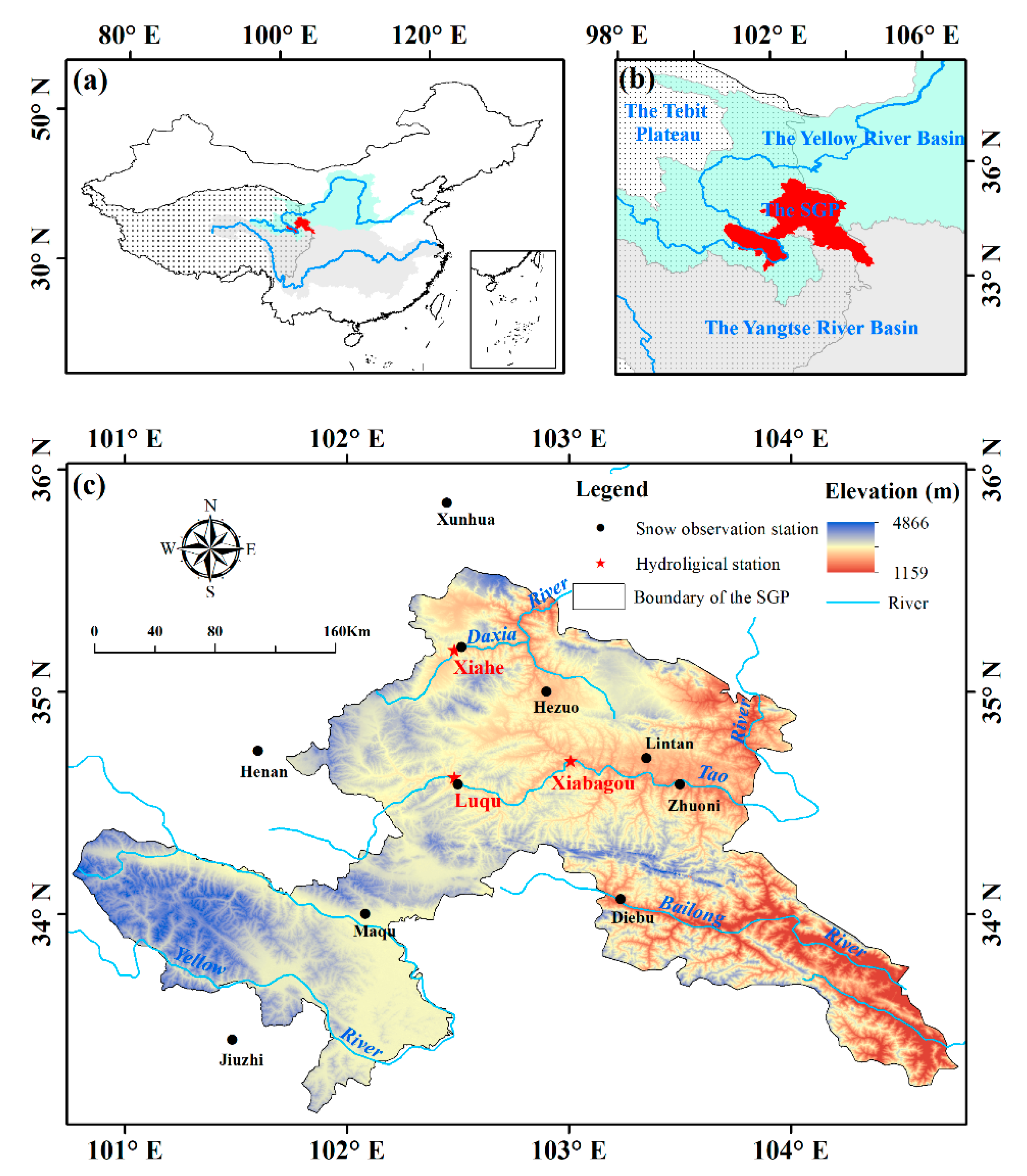
Figure 2.
Schematic diagram of the statistical-based method and the improvement from introducing snow distribution probability for downscaling SD data.
Figure 2.
Schematic diagram of the statistical-based method and the improvement from introducing snow distribution probability for downscaling SD data.

Figure 3.
Evaluation of the improved downscaling method based on the differences from the gauge-based SD observations. and represent the absolute error between the SD data before and after downscaling, respectively. Subplots (a−j) correspond to the gauge stations for snow observation. Names of the stations labeled in the right corners of the plots.
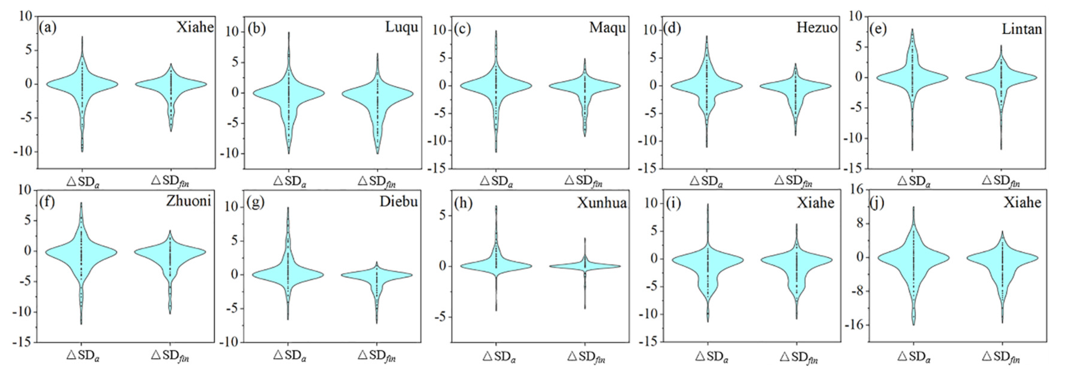
Figure 4.
The spatial distribution of LSSPs on the SGP. Subplots (a–d) are for SD, SCS, SCM, and SCD.
Figure 4.
The spatial distribution of LSSPs on the SGP. Subplots (a–d) are for SD, SCS, SCM, and SCD.
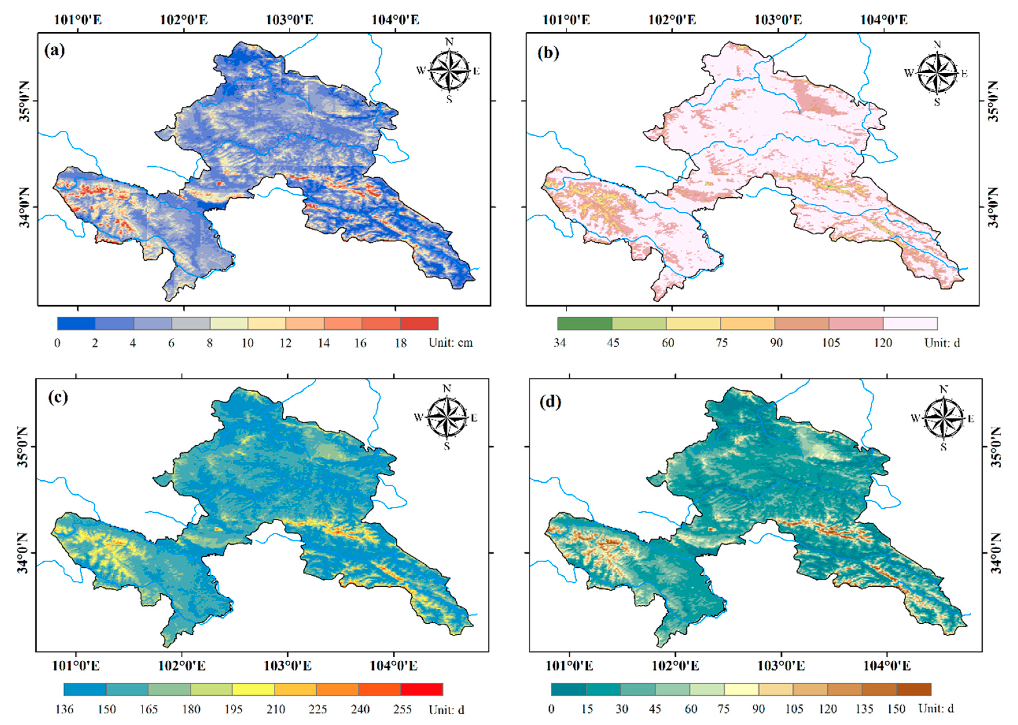
Figure 5.
Multiyear averaged monthly distribution of SD (a) and SCD (b) in SGP (2003–2018).

Figure 6.
Interannual variations of the four selected LSSP indices on the SGP (2003–2018).
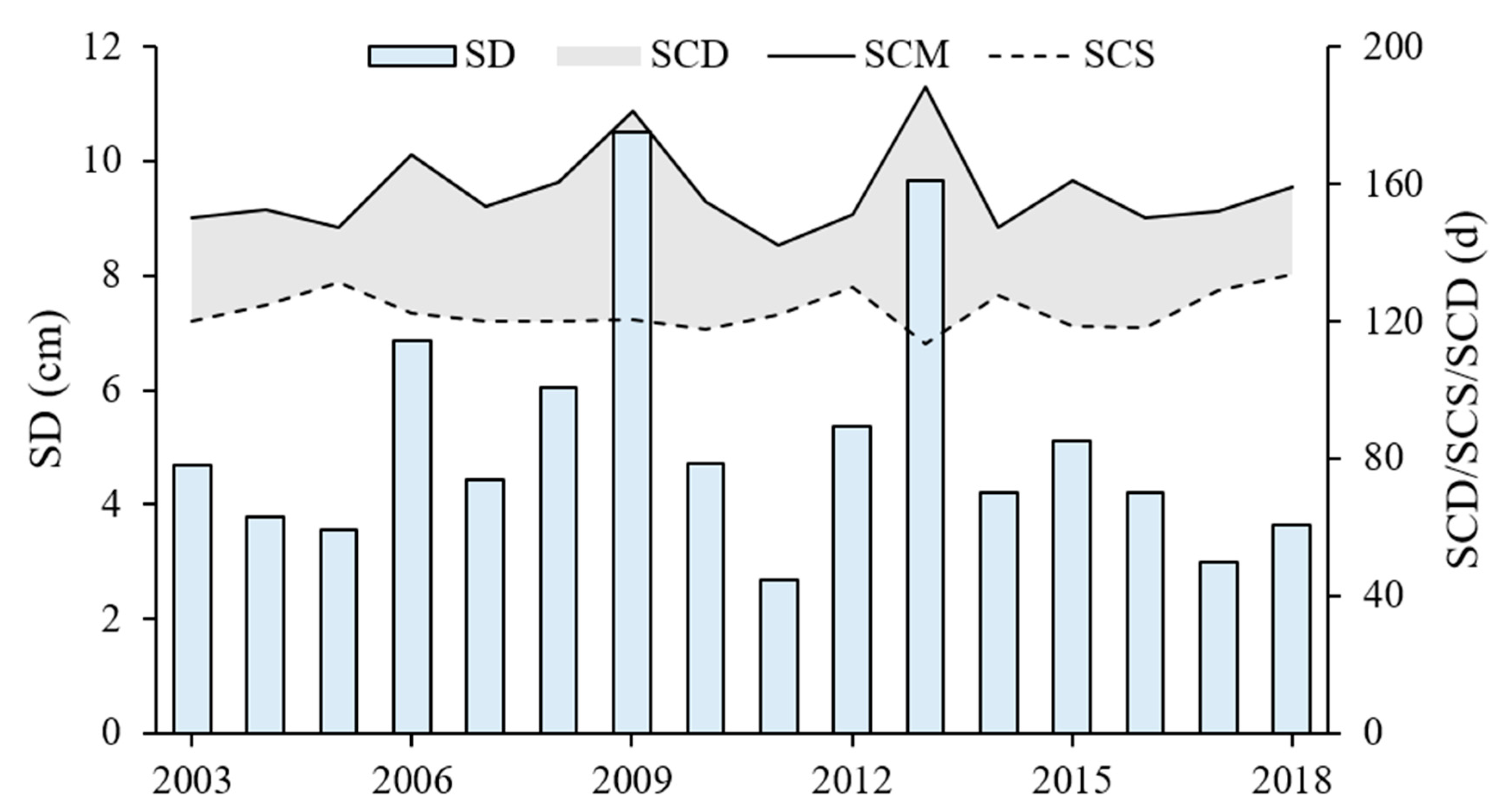
Figure 7.
Spatial variation of the four selected LSSP indices across the SGP (2003–2018). Subplots (a–d) are for SD, SCS, SCM, and SCD in order). “∗” indicates an area with significantly tested LSSP series (p ≤ 0.01). Fan diagrams in the upper left corners of the subplots indicate areal proportions of increasing and decreasing, differentiated using blue and orange, while regional averages are indicated by the white part in the middle.
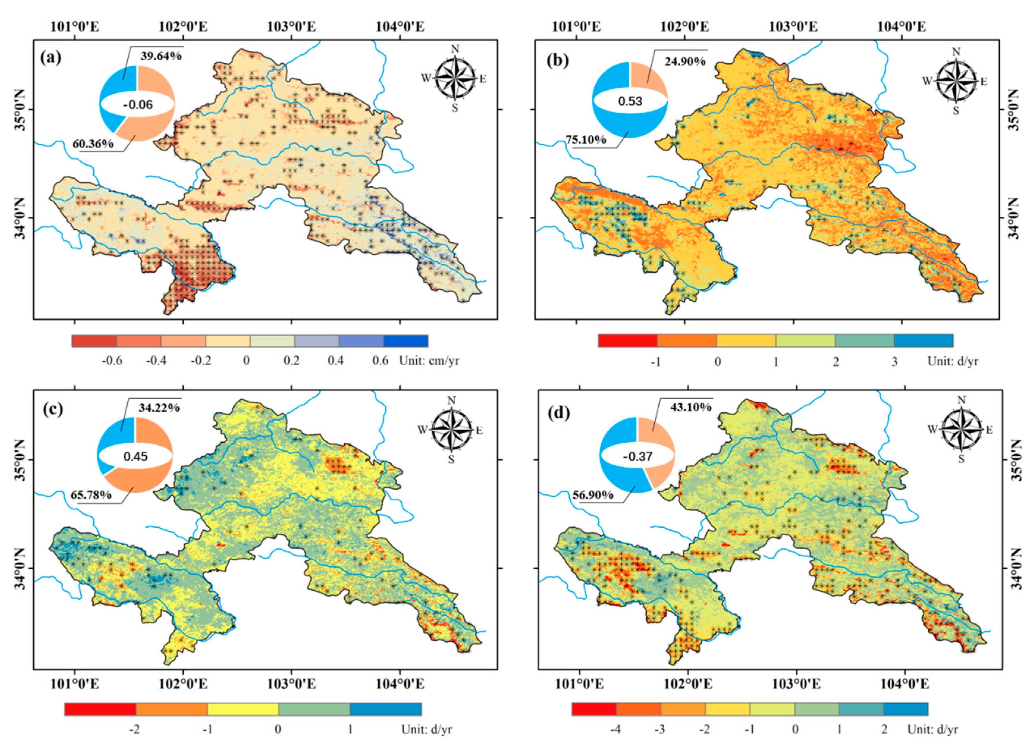
Figure 8.
Reclassification of the three selected topographic factors together with their areal statistics across the SGP. Subplots (a–c) are for altitude, slope, and aspect, respectively.
Figure 8.
Reclassification of the three selected topographic factors together with their areal statistics across the SGP. Subplots (a–c) are for altitude, slope, and aspect, respectively.

Figure 9.
Statistics of LSSP based on terrain. Subplots (a–d), (e–h) and (i–l) correspond to altitude, slope, and aspect, respectively.
Figure 9.
Statistics of LSSP based on terrain. Subplots (a–d), (e–h) and (i–l) correspond to altitude, slope, and aspect, respectively.
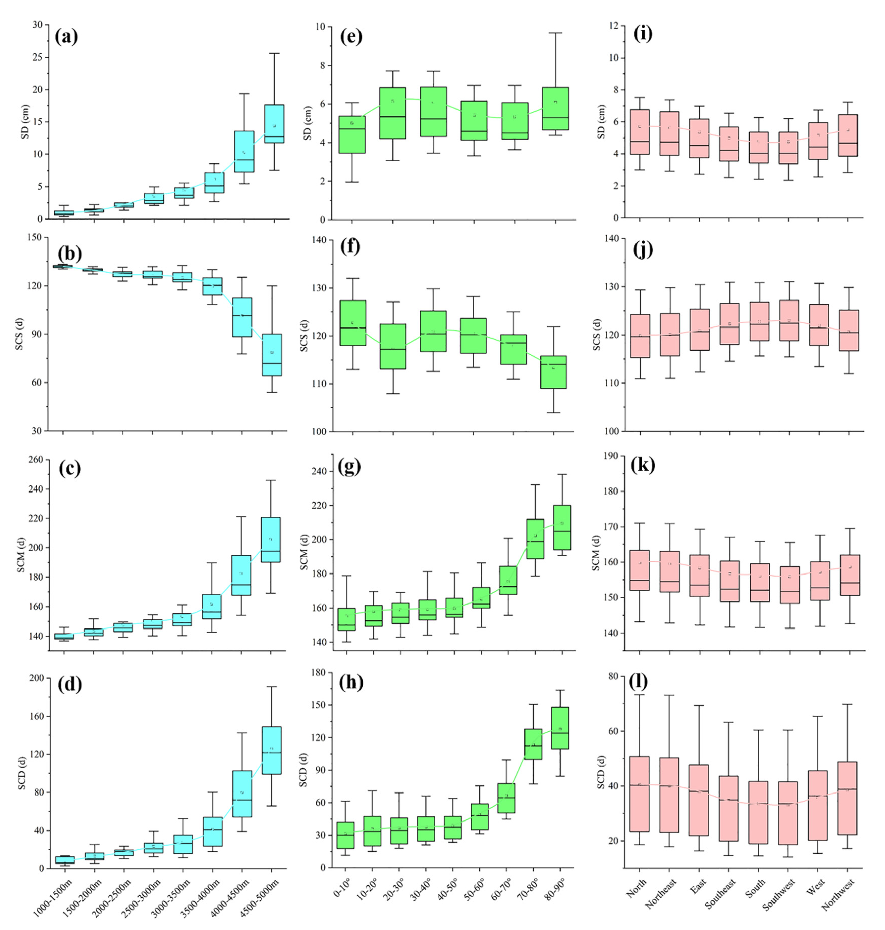
Figure 10.
Quantified annual variation in SD (cm/a), SCS (d/a), SCM (d/a), and SCD (d/a) corresponding to the terrain factors of the SGP. Subplots (a–c) represent zonal statistics based on the reclassified altitude, slope and aspect, respectively.
Figure 10.
Quantified annual variation in SD (cm/a), SCS (d/a), SCM (d/a), and SCD (d/a) corresponding to the terrain factors of the SGP. Subplots (a–c) represent zonal statistics based on the reclassified altitude, slope and aspect, respectively.
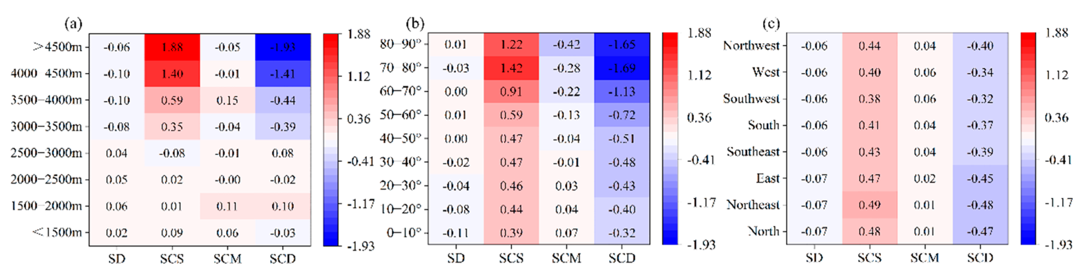
Figure 11.
Significance-based diagnosis of the relationship between LSSP and key climatic factors and their combinations on the SGP. Subplots (a,b) correspond to SD and SCD, respectively. Histograms in the left corners show the top five areas influenced (km2) and NC indicates an area that failed the significance test.
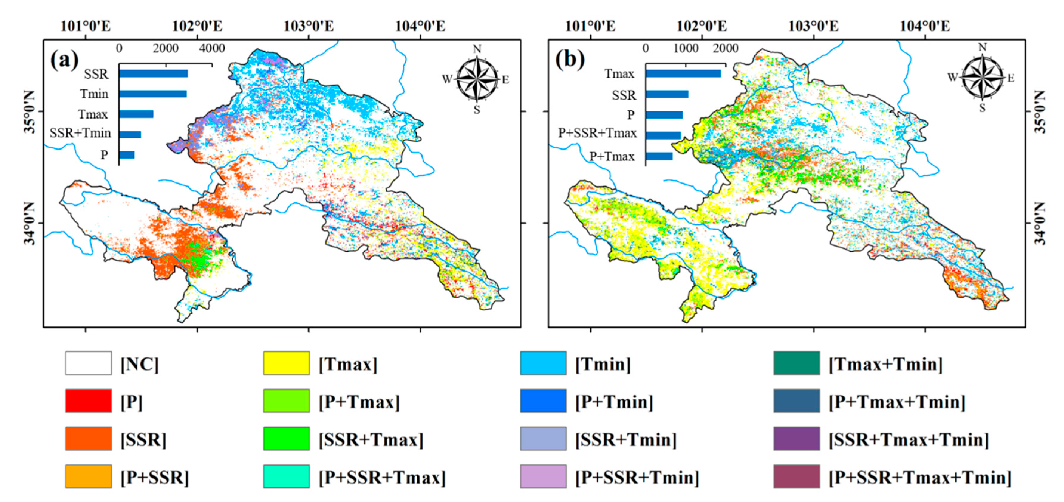
Figure 12.
Spatial distribution of the SD sensitivity to the four climatic factors. Subplots (a–d) correspond to P, SSR, Tmax and Tmin, respectively. Fan diagrams in the upper left corners of subplots indicate the areal proportion of positively or negatively influenced and are differentiated using blue and orange, while the regional averages are the white part in the middle.

Figure 13.
Spatial distribution of SCD sensitivity to the four climatic factors. Subplots (a–d) correspond to P, SSR, Tmax and Tmin, respectively. Fan diagrams in the upper left corners of subplots indicate the areal proportion of positively or negatively influenced and are differentiated using blue and orange, while the regional averages are indicated by the white part in the middle.

Figure 14.
LSSP sensitivity statistics based on combinations of climatic and terrain factors. Subplots (a,b) are altitude-based, (c,d) are slope-based, and (e,f) are aspect-based.
Figure 14.
LSSP sensitivity statistics based on combinations of climatic and terrain factors. Subplots (a,b) are altitude-based, (c,d) are slope-based, and (e,f) are aspect-based.


Table 1.
Significance-based analysis standards for climate driving forces on LSSP.
| Driving Force | t Test-P | t Test-SSR | t Test-Tmax | t Test-Tmin |
|---|---|---|---|---|
| [P] | |t| > t0.01 | |t| < t0.01 | |t| < t0.01 | |t| < t0.01 |
| [SSR] | |t| < t0.01 | |t| > t0.01 | |t| < t0.01 | |t| < t0.01 |
| [P + SSR] | |t| > t0.01 | |t| > t0.01 | |t| < t0.01 | |t| < t0.01 |
| ...... | ...... | ...... | ...... | ...... |
| [P + SSR + Tmax + Tmin] | |t| > t0.01 | |t| > t0.01 | |t| > t0.01 | |t| > t0.01 |
| [NC] | |t| < t0.01 | |t| < t0.01 | |t| < t0.01 | |t| < t0.01 |
Note: t test-P, t test-SSR, t test-Tmax, and t test-Tmin represent the t significance test of LSSP with P, SSR, Tmax, and Tmin, respectively. [P] and [SSR] indicate that LSSP is driven by P or SSR. [P + SSR] indicates that LSSP is driven by both P and SSR. [P + SSR + Tmax + Tmin] means that LSSP is conjointly driven by P, SSR, Tmax, and Tmin. [NC] means nonclimate-driven. There are four key climatic factors and a total of 16 driving force combinations or single factors. Not all of them are listed due to space limitations.
Publisher’s Note: MDPI stays neutral with regard to jurisdictional claims in published maps and institutional affiliations. |
© 2022 by the authors. Licensee MDPI, Basel, Switzerland. This article is an open access article distributed under the terms and conditions of the Creative Commons Attribution (CC BY) license (https://creativecommons.org/licenses/by/4.0/).
Share and Cite
MDPI and ACS Style
Wu, L.; Li, C.; Xie, X.; Lv, J.; Zou, S.; Zhou, X.; Shen, N. Land Surface Snow Phenology Based on an Improved Downscaling Method in the Southern Gansu Plateau, China. Remote Sens. 2022, 14, 2848. https://doi.org/10.3390/rs14122848
AMA Style
Wu L, Li C, Xie X, Lv J, Zou S, Zhou X, Shen N. Land Surface Snow Phenology Based on an Improved Downscaling Method in the Southern Gansu Plateau, China. Remote Sensing. 2022; 14(12):2848. https://doi.org/10.3390/rs14122848
Chicago/Turabian StyleWu, Lei, Changbin Li, Xuhong Xie, Jianan Lv, Songbing Zou, Xuan Zhou, and Na Shen. 2022. "Land Surface Snow Phenology Based on an Improved Downscaling Method in the Southern Gansu Plateau, China" Remote Sensing 14, no. 12: 2848. https://doi.org/10.3390/rs14122848
Note that from the first issue of 2016, this journal uses article numbers instead of page numbers. See further details here.