

Mapping Shrub Coverage in Xilin Gol Grassland with Multi-Temporal Sentinel-2 Imagery

1
State Key Laboratory of Remote Sensing Science, Faculty of Geographical Science, Beijing Normal University, Beijing 100875, China
2
Guangzhou Urban Planning & Design Survey Research Institute, Guangzhou 510060, China
*
Author to whom correspondence should be addressed.
Remote Sens. 2022, 14(14), 3266; https://doi.org/10.3390/rs14143266
Submission received: 5 June 2022
/
Revised: 4 July 2022
/
Accepted: 5 July 2022
/
Published: 7 July 2022
(This article belongs to the Special Issue Remote Sensing and Machine Learning in Vegetation Biophysical Parameters Estimation)
Abstract
:In recent decades, shrubs dominated by the genus Caragana have expanded in a large area in Xilin Gol grassland, Inner Mongolia, China. This study comprehensively evaluated the performances of multiple factors for mapping shrub coverage across the Xilin Gol grassland based on the spectral and temporal signatures of Sentinel-2 imagery, and for the first time produced a large-scale shrub coverage mapping result in this region. Considering the regional differences and gradients in the types and sizes of shrub in the study area, the study area was divided into three subregions based on precipitation data, i.e., west, middle and east regions. The shrub coverage estimation accuracy from dry- and wet-year data, different types of vegetation indices (VIs) and multiple regression methods were compared in each subregion, and the key phenological periods were selected. We also compared the accuracy of four mapping strategies, which were pairwise combinations of zoning (i.e., subregions divided by precipitation) and non-zoning, and full time series of VIs and key phenological period. Results show that the mapping accuracy in a dry year (2017) is higher than that in a wet year (2018). The optimal VIs and key phenological periods show high spatial variability. In terms of mapping strategies, the accuracy of zoning is higher than that of non-zoning. The root mean square error (RMSE), overall accuracy (OA) and recall for ‘zoning + full time series (or + key phenological period)’ strategy were 0.052 (0.055), 76.4% (79.7%) and 91.7% (94.6%), respectively, while for ‘non-zoning + full time series (or + key phenological period)’ strategy were 0.057 (0.060), 75.5% (74.6%) and 91.7% (88.6%), respectively. The mapping using VIs in key phenological periods is better than that of using full time series in the low-value prediction of shrub cover. Based on the strategy of ‘zoning + key phenological period’, the shrub coverage map of the whole region was generated with a RMSE of 0.055, OA of 80% and recall of 95%. This study not only provides the first large-scale mapping data of shrub coverage, but also provides reference for shrub dynamic monitoring in this area.
1. Introduction
Shrub encroachment, a process in relation to degraded grasslands, refers to an increase in shrub cover at the expense of herbaceous vegetation in arid and semiarid grasslands [1]. Shrub encroachment has been reported globally, affecting nearly 10–20% of the arid and semiarid grassland regions [2,3], including western United States [4], southern Africa [5], Mediterranean coast of Europe [6], Australia [7], as well as Inner Mongolia, China [8]. Inner Mongolia is an important animal husbandry base and ecological safety barrier for China. However, shrubs of the genus Caragana, such as C. microphylla Lam., C. korshinskii Kom., C. stenophylla Pojark., and C. intermedia Kuang et H. C. Fu., have expanded into grasslands of Inner Mongolia over recent decades [9]. It was reported that C. microphylla covered 5.07 million hectares of grasslands in the 1980s [10], and the shrub-encroached area in the Xilin River Basin increased by 1.24 times from 1983 to 2011 [11], seriously threatening the economic and ecological stability of this region.
In recent years, there have been a lot of studies on the causes and influences of shrub encroachment in Inner Mongolia. Shrub encroachment is considered a result of the resilience of shrub to climate change, overgrazing and reduced fire frequency by a large number of previous studies, but these studies were mostly based on literature reviews, field sampling experiments with limited samples [2,12,13,14] or several high spatial resolution images [8]. Shrub encroachment has indeed changed the original structure and function of the grassland ecosystem, such as biological diversity, ecosystem productivity and carbon cycle [15,16,17]. However, different studies have given inconsistent results on whether the impact was positive or negative [14,18]. The uncertainty and inconsistency of these studies’ results are mainly caused by the spatial limitation of research methods. More specifically, there are no publicly available large-scale shrub distribution data up to now in Inner Mongolia. Large-scale monitoring of shrub coverage can not only help to comprehensively analyze and simulate the interaction of various factors to shrub encroachment at a regional scale, but also has application significance in modeling global vegetation dynamics, soil erosion, and climate simulation and prediction [19,20,21]. Therefore, mapping fractional shrub cover across Inner Mongolia at a regional scale is urgent to fully understand the mechanism and assess the impacts of shrub encroachment.
However, it is challenging to estimate shrub coverage with remote sensing technologies at regional scale in arid and semiarid grassland [22], especially for Inner Mongolia, due to the following reasons. Firstly, the shrub crown is generally smaller than the spatial resolution of medium-resolution remote sensing data (10–100 m), and its coverage is usually very low with an average of 10–15% [8,23,24,25]. As a result, pixels of medium-resolution are highly heterogeneous and include various cover types, such as grass, soil and shadow. Secondly, it is hard to separate shrubs from grasses because both of them show similar spectral reflectance characteristics of healthy vegetation. For arid areas with obvious dry and rainy seasons, such as the Sahelian savanna, the dry season can serve as an important phenological window to minimize the impact of grasses, based on the fact that grasses barely grow in the dry season while shrubs remain green [23]. However, there is no apparent phenological window in Inner Mongolia, which is characterized by a temperate continental climate; thus, the impact of grasses cannot be neglected. In the face of such a complex and challenging problem mentioned above, the current research for shrub coverage monitoring tends to integrate multi-source information and machine learning methods (e.g., [24,26]).
The purpose of this study is to map the shrub coverage of a large-area grassland in Inner Mongolia using medium spatial resolution remote sensing data. There are a few relevant studies with methods including early multi-angle geometric optical model and spectral mixture analysis [27,28,29] and recent object-oriented classification based on unmanned aerial vehicle (UAV) data [8,30]. Unfortunately, however, due to the abovementioned influence of the shrub-grass-soil mixture, the performance of the multi-angle geometric optical model and spectral mixture analysis in shrub coverage estimation is poor [19,28,31,32], and it is not feasible to use UAV data to estimate shrub coverage over a large area. Therefore, it is a new exploration to use medium-resolution remote sensing data to monitor shrub coverage in Inner Mongolia grassland, which requires full consideration of various factors, selection of effective features, and a comprehensive evaluation of methods and features. First, the diversity of shrub types in Inner Mongolia needs to be considered, which is usually neglected in previous studies. According to the investigation, there are 16 species of Caragana genus shrubs in Inner Mongolia. Instead of growing together, they alternate from west to east, which is the result of their long-term adaptation to drought [33]. These species of Caragana have some differences in ecological and physiological characteristics and have unique responses to climate conditions. Therefore, it is reasonable to divide the research area into several subregions according to climatic characteristics.
Second, features should be selected that minimize grass disturbance and are closely related to shrub coverage. The phenological difference between shrubs and grasses is a crucial feature [28]. A field investigation in the experimental station of Taipusi Banner, Inner Mongolia observed that with the increase of shrub coverage, the spring phenology of shrubs was gradually advanced, and the end time of the growing season was gradually delayed [2]. The seasonal differences between shrubs and grasses in Inner Mongolia might be used to eliminate the effects of grasses and distinguish different shrub coverage. However, since the size, temporal distribution and spatial heterogeneity of seasonal differences in this region are not clear, it is possible to use the complete time series of a year to find the optimal observation time. On the other hand, the phenological differences between shrubs and grasses are mainly due to their differences in water competition [34]. Therefore, analyzing the model performance under different precipitation conditions would provide a reference for future research.
Another important feature closely related to shrub coverage is spectral reflectance. A spectral measurement in Inner Mongolia found that, with the increase of C. microphylla community coverage, the absorption in red band and reflection in near-infrared (NIR) increase, while reflection in short wave infrared (SWIR) band (1600 nm) decreases [28]. The relationship between shrub coverage and spectral signals varies with wavelength depending on the different biochemical and biophysical aspects of shrubs, for example, pigment concentration, water content and lignin cellulose content. In addition, the strength of the relationship between shrub coverage and spectral signals varies with season [35], implying the importance to make full use of the available spectral signals of all wavelengths and all time to discuss their performances on the estimation of shrub coverage. When using surface reflectance and vegetation indices from Landsat data and other predictors, combined with a random forest algorithm to estimate tundra coverage in Arctic Alaska, the most important predictors were the vegetation indices rather than surface reflectance [24], because the value of surface reflectance is small and vulnerable to cloud pollution, while vegetation index is the enhanced signal of vegetation.
According to the above considerations, the objective of this research is to map the Caragana fractional cover in arid and semiarid grassland of Xilin Gol, Inner Mongolia, by using various machine learning algorithms with different types of vegetation index (VI) time series derived from Sentinel-2 data under different precipitation conditions. After collecting a batch of sample sets that cover the whole study area through Google Earth images and UAV, the study area was divided into several subregions by precipitation data, and several key issues were analyzed by subregion: (1) What is the optimal precipitation condition, VIs combination, machine learning algorithm and key phenological period for shrub coverage estimation in each subregion? (2) Among the four mapping strategies based on the pairwise combination of zoning and non-zoning, complete time series, and key phenological periods, which one has the highest accuracy for shrub coverage mapping for the whole study area? This research will not only produce the first Caragana coverage distribution map of a large area with higher spatial resolution of this study area, but also provide some references for future related studies.
2. Study Area and Materials
2.1. Study Area
The study area is located in the central part of Xilin Gol League, Inner Mongolia, China (Figure 1a) with an area of about 59,000 km2. Xilin Gol League is an important part of the interlaced area of agriculture and animal husbandry in northern China. It belongs to the mid-temperate continental semiarid climate, showing characteristics of drought, windy and cold. The annual average temperature is 0–4 °C, and the annual average precipitation is about 300 mm. The precipitation mainly occurs from July to September with a large annual difference, but it maintains the rule of decreasing from east to west in space. In recent years, influenced by climate change, overgrazing and other factors, shrubs have expanded to degraded sandy grassland areas. Caragana is the main shrub genus, of which C. microphylla is one of the most widely distributed species. Part of the Otindag Sandy Land at the south of Abaga Banner is excluded. The study area is mainly typical steppe, while the southern part of Sonid Left Banner is desert steppe.
The daily precipitation data of Abaga and Xilinhot meteorological stations from 2010 to 2019 was provided by China meteorological data sharing service system (Figure 1c–e). The average annual cumulative precipitation at Abaga from 2010 to 2019 is 244 mm, less than 301 mm at Xilinhot, which is consistent with the characteristics of higher precipitation in the east and lower precipitation in the west of Xilin Gol League. According to the multi-year precipitation situation of these two stations (Figure 1c) and the availability of Sentinel-2 data, 2017 and 2018 were selected as a dry year and wet year, respectively, to evaluate the impact of different precipitation conditions on shrub coverage estimation. Figure 1d,e shows the monthly cumulative precipitation of 2017, 2018, and ten-year average at Abaga and Xilinhot station, respectively. In 2017, the drought in Abaga occurred in summer (May–June) and autumn (September–October), while the drought in Xilinhot lasted for a long time from May to July, with less precipitation in September–October. In 2018, the precipitation in Abaga and Xilinhot in July and September was significantly higher than the 10-year average.
2.2. Data Collection and Preprocessing
The remote sensing data used in this study include Sentinel-2 L1C products, precipitation grid data and land cover data. We collected all Sentinel-2 L1C top of atmosphere reflectance (TOA) data for the vegetation growing season (April to October) with less than 70% cloud cover in 2017 and 2018, with a total of 566 images (187 in 2017 and 379 in 2018). L2A surface reflectance data were preprocessed from L1C products by batch atmospheric correction using Sen2Cor professional plug-in and were masked according to the Sentinel-2 QA band. In this study, 10 m and 20 m resolution bands were resampled to 20 m. Then, the VI time series with the 7 day temporal resolution was generated by the maximum value composite (MVC) method. The Savitzky–Golay filter [36] was then used to smooth the raw VI time series to further reduce the residual noise.
Four sets of precipitation reanalysis data were used for climatic zoning of the study area (Table 1). TerraClimate is a global monthly climate and climate water balance dataset based on the world climate dataset [37]. Both GPM_IMERG and GPM_GSMap are from Global Precipitation Measurement (GPM), an international satellite mission jointly built by NASA, JAXA and other international organizations, which is aimed to provide global rain and snow observation every three hours. ERA5 is the fifth-generation European Centre for Medium-Range Weather Forecasts (ECMWF) global climate reanalysis data. It is a data set that combines model data with observation data from all over the world. The above four sets of monthly precipitation data with a period of 2001–2019 were obtained from the Google Earth Engine (GEE) platform and were resampled to 5 km.
Land cover product FROM-GLC10 was used to mask non-shrub type. FROM-GLC10 is produced through a random forest classifier based on the existing 30 m global land cover data and Sentinel-2 data in 2017 on the GEE cloud platform [38]. FROM-GLC10 was resampled to 20 m, and pure pixels of cropland, forest, wetland, water and impervious surface were masked.
2.3. Sample Data Collection and Classification
Sample data with high spatial resolution used in this study include Google Earth images (GE) and aerial photos (AE). The GE samples were collected from May to September between 2015 and 2019 with a spatial resolution about 0.5 m. The total number of GE samples is 20, and the total area is about 0.6 km2. As can be seen from Figure 1b, the distribution of GE samples in the study area is uneven. Therefore, in August 2020, we conducted a one-week UAV flight experiment in the study area and obtained 47 scenes of true-color AE images with a spatial resolution of about 0.05 m, covering a total area of about 7 km2. Orthophotos were then generated from AE images using Agisoft PhotoScan software (version 1.4.4, Agisoft LLC, St. Petersburg, Russia).
The shrubs were extracted from GE and AE images by the object-oriented classification method. Firstly, the image was segmented into objects using a multiresolution segmentation algorithm [39]. The algorithm depends on three parameters: scale, shape and compactness. The shape and compactness parameters were set to 0.1 and 0.5, respectively, through visual judgment, and the scale parameter was set from 50 to 80, according to the shrub canopy size. Secondly, the segmented objects were classified into shrub and non-shrub by the features of brightness/spectral value (brightness and mean bands values), spectral difference value (mean difference to brighter neighbors) and geometric shape (roundness and density). Finally, the shrub classification results were aggregated to 20 m to obtain the shrub coverage sample data (Figure 2).
3. Methodology
3.1. Study Area Zoning
Arid and semi-arid ecosystems are highly dependent on precipitation patterns. Monthly accumulated precipitation data of TerraClimate, GPM_IMERG, GPM_GSMap and ERA5 with 5 km spatial resolution were used to characterize the gradient in the whole region. The precipitation data from 2001 to 2019 were averaged over the years to determine the 12 month monthly accumulated precipitation data. Then, the K-means clustering method was adopted to divide the precipitation data into several clusters. To determine the clustering number, the elbow method was used to calculate the clustering error SSE (Sum of the Squared Errors):
where k is the number of clusters and is the th cluster, is the sample point in and is the mean value of all samples in . As the number of k increases, the degree of aggregation of each cluster will increase, that is, SSE will decrease. The core idea of the elbow method is to select the corresponding k value as the final cluster number when SSE tends to decline slowly.
3.2. Vegetation Indices
We selected nine VIs and divided them into four categories according to greenness, yellowness, moisture and background adjustment to evaluate the influence of different types of VIs on shrub coverage estimation (Table 2). The first category is the greenness index, which directly reflects the greenness of live vegetation, including the Normalized Difference Vegetation Index (NDVI) [40] and Green NDVI (GNDVI) [41]. The value of NDVI is easy to saturate in areas with high vegetation coverage. Studies have shown that the correlation between the green band and chlorophyll concentration is stronger than that of the red band. Therefore, GNDVI was proposed by replacing the red band with the green band in the NDVI formula [41].
The second category is the yellowness index, which reflects the senescence of vegetation, including the Normalized Difference Tillage Index (NDTI) [42] and Normalized Difference Senescent Vegetation Index (NDSVI) [43]. NDTI is based on the unique absorption characteristics of cellulose and lignin in dry vegetation biomass at around 2100 nm. NDSVI is based on the absorption characteristics of moisture content of vegetation in the SWIR band.
The third category is the background-adjusted index, including the two-band Enhanced Vegetation Index (EVI2) [44], Modified Soil Adjusted Vegetation Index (MSAVI) [45] and Normalized Difference Phenology Index (NDPI) [46] and Normalized Difference Greenness Index (NDGI) [47]. EVI2 maintains the low sensitivity to the atmosphere and soil background as EVI through the relationship between blue and red reflectance. MSAVI replaces the constant soil adjustment factor (L) with a self-adjusting L function, which increases the dynamic range of the vegetation signal and further reduces the influence of soil background. NDPI uses linear weighting of three bands to minimize snow and soil background values. The design of NDGI follows NDPI, but replaces NDPI’s SWIR with the green band, thus further reducing the impact of dry vegetation such as hay.
The fourth category is moisture index which reflects the moisture content of vegetation. Normalized Difference Moisture Index (NDMI) [48], similar to NDSVI, also uses the absorption of vegetation moisture content in the SWIR band.
3.3. Regression Methods and Parameterization
Four machine learning regression methods including random forest regression (RFR), support vector regression (SVR), partial least squares regression (PLSR) and gaussian process regression (GPR) were used in this study. RFR is an ensemble learning algorithm constructed by multiple independent decision trees, which has the advantages of high accuracy and good robustness [49]. RFR has two important parameters, one is n_estimators, the number of decision trees, and the other is max_features, the number of randomly selected features on each node [49]. In this study, n_estimators was set to 300, and max_features was adjusted before model training. SVR uses a kernel function to convert the nonlinear problem into a linear problem through mapping input data to high-dimensional feature space [50]. In this study, the kernel function was fixed to the commonly used Gaussian kernel, and parameters C and gamma were adjusted. PLSR transforms the original data into a small number of potential components based on the covariance of collinearity between independent variables and dependent variables [50]. The adjustable parameter of PLSR is n_components, the number of potential components. GPR is an algorithm based on Bayesian probability theory. It is a generalization of Gaussian distribution, in which the output variables of training samples and test sample points are regarded as samples of joint multivariate normal distribution, so the goal of GPR is to fit the distribution of mean function and covariance function of joint multivariate normal distribution [51]. The main parameter of GPR is the covariance kernel function K(x1, x2), which defines the distance between a pair of data points (x1, x2). In this study, we used the common anisotropic square exponential kernel function [51]:
where is the scaling factor, B is the feature number, is the length scale of feature b, which defines the similarity between samples, is Gaussian noise, is the Kronecker symbol. The hyperparameters of kernel function were automatically optimized in the training process.
3.4. Model Training for Shrub Coverage Estimation
3.4.1. General Training and Validation Strategies
After zoning the study area into several subregions using the precipitation grid data, the samples were divided into training samples and test samples in each subregion. The training samples were used for model training and validation accuracy calculation, while the test samples were independent of model training and were used to calculate test accuracy. In the process of the model construction, a five-fold cross-validation strategy was adopted and repeated 20 times. The accuracy evaluation indicators consist of regression accuracy and classification accuracy. The shrub classification result was acquired by classifying the pixels into shrub pixels and non-shrub pixels with a shrub coverage threshold of 0.05. We calculated the root mean square error (RMSE) for regression accuracy, and the overall accuracy (OA), precision and recall for classification accuracy.
3.4.2. Key Phenological Period Evaluation
Both RFR and GPR can output the evaluation results of feature importance. The feature importance derived from RFR is measured by the degree of reduction of mean square error after the introduction of feature variables. The feature importance of GPR is calculated by the inverse of . The greater the inverse of , the greater the relative importance of feature b.
To evaluate the key phenological period, this study integrated the results of feature importance evaluation returned by RFR and GPR. For each VI time series, 100 RFR and 100 GPR models were established, respectively. The final feature importance of RFR is the average value of the feature importance scores from the 100 models, and the final feature importance of GPR is the frequency of the top five reverse of . Finally, the integrated ranking of feature importance is the average of the importance score ranking of RFR and the importance frequency ranking of GPR. A larger ranking value means higher feature importance, indicating that the corresponding phenological period is more critical for shrub coverage estimation.
3.4.3. Mapping Strategies for the Whole Study Area
The experiment design of shrub coverage estimation for the study area using Sentinel-2 time series data includes the following steps. Firstly, in each subregion, a single VI time series and a single regression method were used to build models. Then, the accuracy of these models and the importance of all features were compared to find the optimal VIs, machine learning algorithm and key phenological period for each subregion. Finally, four shrub coverage mapping strategies were constructed and compared, and the optimal mapping strategy was selected to plot the shrub coverage distribution map in the whole study area. The four mapping strategies are as follows.
- Strategy1 (Stgy.1): zoning + full time series of VIs, that is, the full time series of optimal VIs are used to construct the model in each subregion, and then the partition results are combined into the whole region results.
- Strategy2 (Stgy.2): zoning + key phenological period, that is, the top five key phenological periods of optimal VIs are selected to construct the model in each subregion.
- Strategy3 (Stgy.3): non-zoning + full time series, that is, all the optimal VIs time series in the subregions are put together to construct the model with all the training samples.
- Strategy4 (Stgy.4): non-zoning + key phenological period, that is, the top five key phenological periods of all optimal VIs selected in each subregion are put together to construct the model.
4. Results
4.1. Zoning Result of the Study Area
K-means clustering number selection and final clustering results of four sets of precipitation data are shown in Figure 3. From the scatter plot of SSE and cluster number k, it can be seen that as k increases, the SSEs of the four sets of precipitation data gradually decrease, indicating that there is a spatial gradient distribution pattern for precipitation. Specifically, when k increases from 1 to 3, SSE shows a large decrease. Then, when k increases from 3, the decline of SSE obviously tends to be slow, so the final cluster number k is set to 3, that is, the study area is divided into three subregions. Although the clustering results of the four sets of precipitation data are slightly different, they all show an obvious gradient increasing from west to east (Figure 3b). The multi-year averaged monthly precipitation curves show that the precipitation differences in the three subregions mainly occur from May to September, and the differences reach the maximum in July (Figure 3c).
To improve the reliability of the regional zoning results, the voting method was used to integrate the clustering results of four sets of precipitation data. The final classification category of a pixel is determined by the category with the largest proportion. Finally, the whole study area was divided into three subregions from west to east, namely West, Middle and East, respectively (Figure 4a). The distribution of training samples and test samples in each subregion is also shown in Figure 4a. Considering that there are fewer samples in the East, no test samples are set in this subregion. Figure 4b shows the histogram distribution of shrub coverage of all sample pixels in the three subregions. It can be seen that the average shrub coverage of the samples in each subregion gradually increases from west to east, with an average shrub coverage of 0.076 in the West, 0.087 in the Middle and 0.157 in the East.
4.2. The Optimal Factors in Each Subregion
In each subregion, the shrub coverage regression model was established by using the time series of each VI combined with each regression method under different precipitation conditions, and then the performances of different factors were compared with validation accuracy and test accuracy. These factors include precipitation conditions, VIs and regression methods. Results are shown in Figure 5 for the West subregion, Figure 6 for the Middle subregion and Figure 7 for the East subregion.
In the West subregion (Figure 5), the validation and test accuracies are consistent for the dry year (2017) and wet year (2018), and the accuracies of VIs in the dry year are higher than those in the wet year. The differences in validation accuracies of the nine VIs are very small, but the test accuracies of NDTI and NDGI in the dry year are significantly higher than those of the other VIs. SVR and RFR outperform PLSR and GPR in shrub coverage estimation. The test accuracy of SVR (RMSE = 0.052) is slightly higher than that of RFR (RMSE = 0.057), while the validation accuracy of RFR (RMSE = 0.051) is significantly higher than that of SVR (RMSE = 0.071). This result suggests that the method of RFR is more suitable for shrub coverage estimation in the Western subregion.
In the Middle subregion (Figure 6), the role of dry and wet years was analyzed by the test accuracy considering the significant differences in test accuracies. Results show that the accuracies of VIs except for NDTI in the dry year are higher than those in the wet year. For the accuracy comparison of VIs, NDMI, NDPI, EVI2 and MSAVI in the dry year and NDTI in the wet year show higher validation and test accuracies. For comparison of accuracies of the regression methods, RFR has the highest validation accuracy, while SVR has the highest test accuracy. However, SVR and RFR have little difference in accuracy for dry year.
In the East subregion (Figure 7), some VIs show slightly higher validation accuracies for RFR and GPR methods in wet years than in dry years, while SVR and PLSR have significantly higher accuracies in the dry year than in the wet year. Generally, the accuracy of dry year is higher than that of wet year in the East subregion. NDMI, NDPI, EVI2 and MSAVI in the dry year and NDTI in the wet year have higher validation accuracy, which is similar to the Middle subregion. For comparison of the regression methods, RFR achieves the highest accuracy in this subregion.
We summarized the optimal factors for the three subregions. Firstly, the accuracies of VIs in the dry year are higher than those in the wet year except for NDTI. Secondly, the results of the three subregions show that the accuracy of RFR is relatively higher than the other three regression methods. Lastly, the optimal VIs for the West subregion are NDTI and NDGI in the dry year, and the optimal VIs for the Middle and East subregions are NDMI, NDPI, EVI2 and MSAVI in the dry year and NDTI in the wet year. Considering that NDPI, EVI2 and MSAVI are background adjustment indices with similar effects, we selected MSAVI for shrub coverage mapping because the vegetation is sparse in arid and semiarid areas and soil background has a greater impact on VIs.
4.3. The Key Phenological Periods in Each Subregion
Figure 8 shows the ranking results of the feature importance of time series in each subregion obtained from RFR and GPR. Based on the ranking values, we selected the key phenological periods in dry and wet years for each subregion. In the West subregion, early April in both dry and wet years is one of the key phenological period, and the other key phenological periods are in summer, including mid-July in the dry year and late June in the wet year. In Middle subregion, early July and late October are the key phenological periods of dry and wet years. In the East subregion, late September is a key phenological period, and another key phenological period is advanced from mid-June in the dry year to late May in the wet year. The key phenological period in early summer of the wet year has a potential tendency to be ahead of that in the dry year.
We compared the key phenological periods of the three subregions. The key phenological periods in the summer of the dry year show an obvious trend of advance from west to east, which are mid–late July in the West subregion, early July in the Middle subregion and mid–late June in the East subregion, respectively. However, there is no such spatial trend in the wet year.
4.4. Comparison of Shrub Coverage Mapping Strategies
In this section, we compared the accuracy of the four mapping strategies and selected the best one for shrub coverage mapping in the entire region. Table 4 lists the average of validation accuracy and test accuracy of four mapping strategies. It can be observed from Table 4 that the validation accuracy of the four mapping strategies are similar, indicating that zoning and non-zoning, full time series and key phenological periods have little impact on model training. Among the validation accuracy of the four strategies, RMSE is 0.050, OA is around 83%, about 96% of the shrub pixels are correctly classified and the probability of being correctly classified as shrub pixels is about 80%. However, the test accuracy of the four mapping strategies varies greatly. As can be observed from Table 4, the RMSE of zoning mapping is lower than that of non-zoning mapping, and OA, precision and recall of zoning are also significantly higher than those of non-zoning, so the accuracy of zoning mapping is higher than that of non-zoning mapping. However, the accuracy of the full time series and key phenology depends on zoning or not. Among the four strategies, Stgy.1 holds the smallest RMSE (0.052) and Stgy.4 has the largest RMSE (0.060), while Stgy.2 presents the highest classification accuracy and Stgy.4 has a relatively low classification accuracy.
The predicted shrub coverage based on the four mapping strategies and the true coverage of the validation samples are all distributed near the 1:1 line (Figure 9a–d), showing the high prediction accuracy. However, the scatter plots of the test samples show a tendency of overestimation in the low-value areas and underestimation in the high-value areas (Figure 9e–h), and this trend is more obvious in the non-zoning mapping strategy. To compare the ability of the four mapping strategies to distinguish shrubs from grasses, the average predicted coverage of non-shrub pixels was counted as the Mean0 index (Table 4). Results show that the Mean0 of the validation samples predicted by the four strategies are close (0.023–0.026), while the Mean0 of test samples predicted by full time series strategy is higher than that predicted by the key phenological period strategy, indicating that the full time series strategy tends to overestimate non-shrub pixels. Stgy.2 has the smallest Mean0 value (0.045) and Stgy.3 has the largest one (0.058).
From the regression accuracy and classification accuracy results of the test samples, it can be concluded that the accuracy of the zoning mapping strategy is higher than that of the non-zoning, and the VIs in the key phenological periods strategy is better than the full VI time series in terms of low value prediction performance. Among the four mapping strategies, Stgy.2 (zoning + key phenological period) shows the highest test accuracy, Therefore, Stgy.2 was selected to produce the shrub coverage map of the whole study area at a spatial resolution of 20 m (Figure 10, upper).
From the mapping result, the maximum shrub coverage is less than 0.45, 87% of the areas have shrub coverage less than 0.1 and only 2.5% of the areas have shrub coverage greater than 0.15. The areas with shrub coverage greater than 0.15 are mainly distributed at the edge of the Otindag Sandy Land in the east of Sonid Left Banner, the Xilin River basin in Xilinhot, and the hills and mountains in the southeast of the study area. In terms of spatial distribution, the distribution of shrub coverage follows the precipitation gradient, showing an increasing trend from west to east. From the comparison between the high spatial resolution images and predicted shrub coverage of test samples (Figure 10 bottom, locations A–E), it can be found that the mapping result can accurately extract the spatial distribution of shrubs; however, it is easy to identify the vegetation and mountain forest around the water as shrubs.
5. Discussion
5.1. Reliability of Shrub Coverage Mapping Result
Based on spectral information and phenological information, this study used the latest Sentinel-2 data and machine learning algorithms to estimate the coverage of Caragana in the Xilin Gol grassland of Inner Mongolia. The RMSE of the validation samples and the test samples were 5% and 5.5%, respectively, indicating the reliability of the shrub coverage mapping results. The results of this study were not compared with other global tree cover products such as MOD44B, because most of these products are designed for forest areas rather than grasslands, which only provide information on the cover of tall trees in arid and semiarid areas, and ignore dwarf shrubs [23]. Moreover, the spatial resolution of global tree productions is too rough, and the error is large in arid and semiarid areas with sparse vegetation. The spatial resolution of the distribution of shrub coverage in this study is 20 m, which can provide more accurate and detailed information.
As far as we know, the result of this study is the first large-scale and high spatial resolution data on the distribution and coverage of Caragana in Inner Mongolia. Since there is no other reference data, we can only verify our results from the text descriptions in previous studies. Results show that the coverage of Caragana increases from west to east in Xilin Gol grassland, which is consistent with the local precipitation gradient, and the areas with higher coverage (>15%) are mainly distributed in the Xilin River Basin and the edge of Otindag Sandy Land. In the investigation of C. microphylla, C. intermedia and C. korshinskii communities, it was found that the abundance of C. microphylla gradually increased from the east of Xilinhot to the west, reached the maximum in Xilinhot, and then began to decline [53], which confirmed the reliability of the spatial distribution result of this study. In general, the model of this study shows good accuracy and provides a reliable estimation of Caragana shrub coverage for the Xilin Gol grassland in Inner Mongolia. Moreover, a large-scale UAV field experiment has accumulated a number of reliable field measured data for this region, which can provide important reference information for future study of grassland ecosystem and shrub expansion in this region.
5.2. Significance of Zoning and Feature Selection
In this study, precipitation grid data were used to divide the study area into three subregions, and then the accuracy of the two mapping strategies of zoning mapping and non-zoning mapping were compared. We found that the accuracy of zoning mapping was higher than that of non-zoning mapping, presenting that the slope of the referenced coverage and the predicted coverage of test samples for zoning mapping strategy was closer to 1, while non-zoning mapping tended to predict the mean value for all test samples (Figure 9). In the shrub component mapping research in North America, the importance of zoning was also considered by using climate data to divide the study area into three subregions [25]; however, the mapping results of zoning and non-zoning were not compared. Arid and semiarid grasslands are highly dependent on climatic conditions and have distinct vegetation heterogeneity. We have verified through experiments that a single model cannot well reflect the spatial distribution characteristics of shrubs in this region, and it is easy to cause the prediction result to be smoothed around the mean value. Only the models established under different climatic conditions can accurately reflect the unique response of different types of shrubs to the climatic conditions.
The optimal VI combination of each subregion is different. For the driest West subregion, the optimal VIs are NDTI and NDGI, while for the wetter Middle and East subregions, the optimal VIs are NDMI, NDTI and background adjustment index. The difference in the optimal VI combination of the three subregions indicates that there may be differences in the mixed components of shrub and grass between these subregions. In the field UAV sampling experiment, we also found the different Caragana growth statuses in the West and Middle subregions (Figure 11). Caragana stenophylla is the dominant species in the West subregion, where the herbaceous coverage is low. C. microphylla, with a larger canopy size, is mainly distributed in the Middle subregion, where herbaceous plants grow well and are highly mixed with C. microphylla. The spatial pattern of Caragana species substitution from east to west is closely related to their relationship with water supply [33]. Therefore, it is necessary to zone the study area when monitoring the shrub coverage of the Xilin Gol grassland at a large scale.
This study also found that the accuracy of selecting important features for shrub coverage estimating is slightly higher than the accuracy of using all features, especially for zoning mapping strategies (Table 4). The advantage of important features over all features is mainly reflected in the prediction of low value areas. It can be seen from Table 4 that the average coverage of non-shrub pixels predicted by important features is lower than that predicted by all features, which indicates that using all features is more likely to cause overestimation of low value areas and detect more false-positive shrubs. That is because inputting more unimportant variables will introduce more noise and cause a high correlation between variables, which may reduce the stability and interpretability of the model [54]. Therefore, it is important to filter features before the shrub coverage model training and find a simplified feature subset that can balance accuracy and model interpretability. On the other hand, from the perspective of computing efficiency, although the accuracy after feature selection is not significantly improved, a smaller feature subset can reduce the computing time, which is very efficient for large sample learning.
5.3. Spatial Variability of Optimal VIs and Key Phenological Period
Interestingly, this study found spatial variability of optimal VIs in three subregions. In the humid Middle and East subregions, the VIs that perform well are mainly the background-adjusted index and the moisture index. This may be because of the larger interference of background factors like grasses in humid areas. In the arid West subregion, the vegetation index that performs better is the NDGI, excluding other background-adjusted indices. It may be because the introduction of the green band improves the sensitivity to low chlorophyll concentration. In addition, the three band combination eliminates the influence of background, so it outperforms GNDVI, which also introduces green band. This study also discovered the potential of an uncommon VI in shrub coverage monitoring: NDTI. This index is selected as the optimal VI by the three subregions. NDTI combines SWIR1 (1610.4 nm) and SWIR2 (2185.7 nm) and was originally designed to monitor the residue coverage after farming and harvesting. We further found that NDTI in early April showed a significant negative correlation with shrub coverage. A previous study used MODIS reflectance data and a multiple regression model to estimate woody plant coverage of the central Texas savanna and found that woody plant coverage had a strong negative linear relationship with the annual minimum reflectance of MODIS band 6 (1628–1652 nm) and band 7 (2105–2155 nm), and the absolute value of regression coefficient of band 6 was greater than that of band 7 [55], indicating that NDTI’s negative correlation relationship to shrub coverage in this study may be due to the difference of radiation absorption of woody plants in these two SWIR bands. The reflectance characteristics of the SWIR band are closely related to the moisture, cell structure, lignin and cellulose content of vegetation, and the potential of the SWIR band in wood vegetation coverage prediction has also been discovered in other studies [56]. In the future, we can use hyperspectral technology to conduct ground spectral measurement experiments to explore the radiation characteristics of woody plants in the SWIR band.
The time acquisition of features is very crucial for model learning because the introduction of key phenology can exclude the interference of the background signal and improve the differentiation of target and background. In this study, we separately modeled the data for the dry year and wet year and found that the accuracy of the dry year is higher than that of the wet year, thanks to the stronger drought resistance of shrubs than grasses [12]. This finding has also been concluded in other studies [55,57]. The results of the feature importance evaluation showed that June to July and September were two key phenological windows for shrub monitoring in Xilin Gol grassland. However, it should be noted that the phenological window presented a gradient trend in space. Specifically, the key summer phenological windows of the three subregions advanced from west to east, from late July to early July, and then to late June. The gradient difference was about half a month. Therefore, when monitoring shrub coverage in large areas in the future, we should fully consider the geographical gradient of phenology and set up multiple important phenological windows or use complete time series.
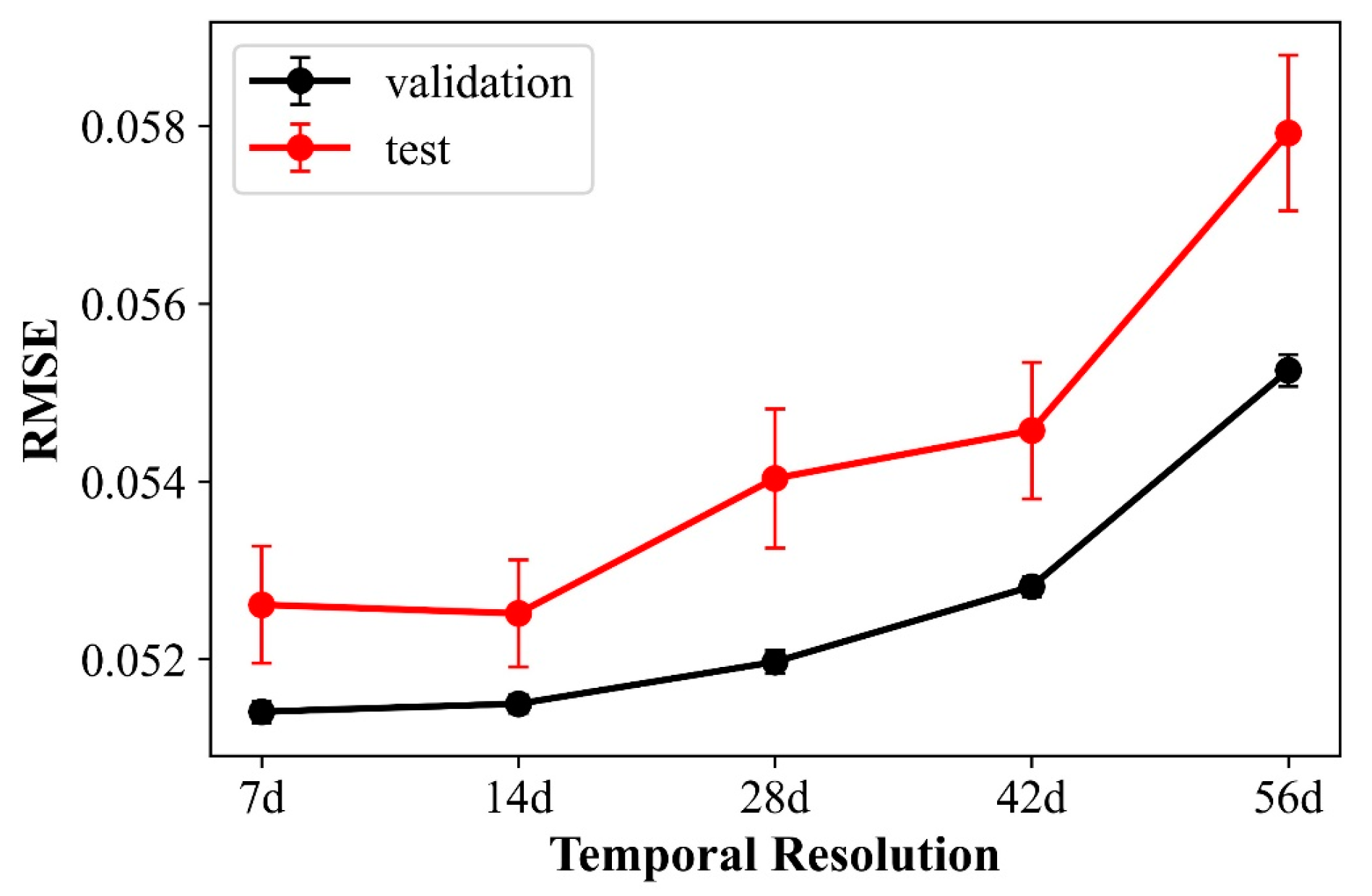
To further analyze the sensitivity of shrub monitoring accuracy to the time resolution of the VI time series, we averaged the VI time series with 7 day (7 d) resolution to generate new time series with the different temporal resolutions and then used the Stgy.1 to predict shrub coverage. The final result is shown in Figure 12. There is no significant difference in the accuracy of time series with resolutions of 7 d and 14 d. When the temporal resolution increases from 14 d, the mean value and standard deviation value of RMSE increase, which indicates that the accuracy and stability of the model decrease. The turning point of 14 d resolution is consistent with the phenological gradient of the three sub-regions mentioned above. Therefore, it is recommended to use a time series with a half-month resolution for shrub coverage monitoring in this region.
5.4. Uncertainties and Deficiencies
Both quantitative evaluation (Figure 9, Table 4) and visual evaluation (Figure 10) indicated that the random forest model trained by the VI time series could quantitatively describe the spatial distribution of Caragana coverage in Xilin Gol grassland. Nevertheless, some uncertainties and deficiencies of this study need to be mentioned. The first is the uncertainty of the results. The RMSE of the final model is between 5% and 5.5%, while the coverage mapping results show that the area below 5% coverage accounts for half, indicating that half of the study area has uncertainty. The scatter plot of the test samples shows that the shrub coverage tends to be overestimated at low values and underestimated at high values (Figure 9), which is very similar to other studies using regression modeling for shrub coverage mapping [24,25,55,57]. The overestimation of the low value area is mainly due to the method of sample data collection. The shrub canopy is radially distributed, and other vegetation generally grows under the canopy. However, we define the shrub coverage as the proportion of the vertical projection area of the shrub canopy, ignoring other vegetation below the canopy. The underestimation of the high-value area is mainly caused by the random sampling strategy. Due to the scattered distribution of shrubs in the Xilin Gol grassland, the coverage itself is not high. There are fewer pixels of high coverage in the training sample, and the coverage distribution is uneven. A possible way to solve this problem is to balance the coverage distribution of samples, but it needs to have a certain prior knowledge of the target distribution in the study area, which is difficult to obtain in large-area studies. Other uncertain results appear in river vegetation mixed with water bodies, agricultural land and mining areas, and in forest land in mountainous areas.
There are three main deficiencies in this study. First, this study simply uses the precipitation grid data with a coarse spatial resolution to divide the study area into subregions. In the future, soil texture, soil moisture and other data can be used to divide the study area under the premise of data availability. Second, this study did not fully utilize Sentinel series data, such as exploring the capability of the red edge band of Sentinel-2 data in shrub coverage monitoring and combining the multi-source information provided by Sentinel-1 SAR data. However, the Sentinel-1 C band is very sensitive to the impact of surface roughness, especially in areas with sparse vegetation [56]. Therefore, how to effectively combine the radar information of Sentinel-1 with the spectral information of Sentinel-2 for shrub coverage monitoring in arid and semiarid regions is a challenging task for the future. Third, the spatial distribution of samples is uneven, and there are fewer samples in the East subregion, which leads to the uncertainty of the results in the east. In the future, we can collect more samples from the eastern region to improve the reliability of the results.
6. Conclusions
A high spatial resolution shrub coverage map (20 m) in the Xilin Gol grassland was generated based on Sentinel-2 spectral and temporal signatures. This study is the first attempt to use high spatial and temporal resolution satellite images to estimate shrub coverage on a large scale. We proposed the following approach to identify and estimate the coverage of shrubs of the genus Caragana considering the interactive spatial, temporal and spectral features. Firstly, the precipitation data were used to divide the study area into similar climate zones, which was helpful to distinguish the characteristics of shrub species and structure. Through the time series data of the adjacent dry and wet years, the key phenological periods of each zone were selected to highlight the growth differences between shrubs and grass. In terms of spectral features, machine learning algorithms were used to select the VIs, which could reflect the spectral difference among shrubs, grass and soil. The performance of different precipitation conditions, different types of VIs and different regression methods in shrub coverage monitoring was fully compared region by region. Moreover, the feature importance evaluation was used to find that the key phenological periods presented an advanced trend from west to east. Different from previous studies, this study also compared the differences between zoning mapping and non-zoning mapping, mapping using all features and mapping using important features, and found that the accuracy of zoning mapping is significantly higher than that of non-zoning mapping. The RMSE, OA, precision and recall for the ‘zoning + full time series (or + key phenological period)’ strategy were 0.052 (0.055), 76.4% (79.7%), 80.0% (81.5%) and 91.7% (94.6%), respectively, while for the ‘non-zoning + full time series (or + key phenological period)’ strategy were 0.057 (0.060), 75.5% (74.6%), 79.2% (80.1%) and 91.7% (88.6%), respectively. The important feature mapping performs better in low value prediction than all feature mapping. However, due to the influence of vegetation beneath the shrub canopy in arid and semiarid areas, the overall woody cover is overestimated in low value and is underestimated in high value. In spite of this uncertainty, the mapping result based on Sentinel-2 imagery provides more accurate information on shrub coverage. The shrub coverage map and UAV samples data provided by this research can serve as a baseline map to not only explore the historical distribution and future changes of shrub coverage, but also analyze the impact of shrub expansion on the ecosystem, environment and economy.
Author Contributions
Conceptualization, X.C. (Xin Cao), L.G. and X.C. (Xuehong Chen); methodology, L.G., X.C. (Xuehong Chen) and Q.H.; software, L.G. and C.Z.; validation, L.G., X.C. (Xihong Cui) and C.Z.; formal analysis, L.G. and X.C. (Xin Cao); investigation, L.G., X.C. (Xin Cao) and C.Z.; resources, Q.H. and C.Z.; data curation, L.G. and C.Z.; writing—original draft preparation, L.G.; writing—review and editing, X.C. (Xin Cao) and X.C. (Xuehong Chen); supervision, X.C. (Xin Cao), X.C. (Xuehong Chen), Q.H. and X.C. (Xihong Cui); project administration, X.C. (Xin Cao); funding acquisition, X.C. (Xin Cao). All authors have read and agreed to the published version of the manuscript.
Funding
This research was funded by the National Natural Science Foundation of China, grant number 41571406.
Data Availability Statement
Sentinel-2 L1C images are available at Copernicus Open Access Hub (https://scihub.copernicus.eu/dhus/#/home (accessed on 3 June 2022)). The meteorological data are provided by China meteorological data sharing service system (http://data.cma.cn/ (accessed on 3 June 2022)). Four sets of precipitation reanalysis data can be obtained from the Google Earth Engine platform (TerraClimate data, https://developers.google.com/earth-engine/datasets/catalog/IDAHO_EPSCOR_TERRACLIMATE?hl=en (accessed on 3 June 2022); GPM_IMERG, https://developers.google.com/earth-engine/datasets/catalog/NASA_GPM_L3_IMERG_MONTHLY_V06?hl=en (accessed on 3 June 2022); GPM_GSMap, https://developers.google.com/earth-engine/datasets/catalog/JAXA_GPM_L3_GSMaP_v6_reanalysis?hl=en (accessed on 3 June 2022); ERA5 data, https://developers.google.com/earth-engine/datasets/catalog/ECMWF_ERA5_LAND_MONTHLY?hl=en (accessed on 3 June 2022)). The sources and spatial resolutions of Google Earth images are provided by DigitalGlobe (https://discover.digitalglobe.com/ (accessed on 3 June 2022)). Land cover product FROM-GLC10 data are provided by the Department of Earth System Science of Tsinghua University (http://data.ess.tsinghua.edu.cn/fromglc2017v1.html (accessed on 3 June 2022)).
Conflicts of Interest
The authors declare no conflict of interest.
References
- Van Auken, O.W. Causes and consequences of woody plant encroachment into western North American grasslands. J. Environ. Manag. 2009, 90, 2931–2942. [Google Scholar] [CrossRef] [PubMed]
- Fan, Y.; Li, X.; Huang, H.; Wu, X.; Yu, K.; Wei, J.; Zhang, C.; Wang, P.; Hu, X.; D’Odorico, P. Does phenology play a role in the feedbacks underlying shrub encroachment? Sci. Total Environ. 2019, 657, 1064–1073. [Google Scholar] [CrossRef] [PubMed]
- Tu, Y.; Liu, Y.; Zhu, Y.; Yang, X.; Zhang, K. Effects of shrub encroachment in Xilin Gol Steppe on the species diversity and biomass of herbaceous communities in shrub interspaces area. J. Beijing For. Univ. 2019, 41, 57–67. [Google Scholar] [CrossRef]
- Knapp, A.K.; Briggs, J.M.; Collins, S.L.; Archer, S.R.; Bret-Harte, M.S.; Ewers, B.E.; Peters, D.P.; Young, D.R.; Shaver, G.R.; Pendall, E.; et al. Shrub encroachment in North American grasslands: Shifts in growth form dominance rapidly alters control of ecosystem carbon inputs. Glob. Chang. Biol. 2008, 14, 615–623. [Google Scholar] [CrossRef]
- O’Connor, T.G.; Puttick, J.R.; Hoffman, M.T. Bush encroachment in southern Africa: Changes and causes. Afr. J. Range Forage Sci. 2014, 31, 67–88. [Google Scholar] [CrossRef]
- Maestre, F.T.; Bowker, M.A.; Puche, M.D.; Belén Hinojosa, M.; Martínez, I.; García-Palacios, P.; Castillo, A.P.; Soliveres, S.; Luzuriaga, A.L.; Sánchez, A.M.; et al. Shrub encroachment can reverse desertification in semi-arid Mediterranean grasslands. Ecol. Lett. 2009, 12, 930–941. [Google Scholar] [CrossRef]
- Fensham, R.J.; Fairfax, R.J.; Archer, S.R. Rainfall, land use and woody vegetation cover change in semi-arid Australian savanna. J. Ecol. 2005, 93, 596–606. [Google Scholar] [CrossRef]
- Cao, X.; Liu, Y.; Liu, Q.; Cui, X.; Chen, X.; Chen, J. Estimating the age and population structure of encroaching shrubs in arid/semiarid grasslands using high spatial resolution remote sensing imagery. Remote Sens. Environ. 2018, 216, 572–585. [Google Scholar] [CrossRef]
- Guo, J.; Chen, S.; Xu, B.; Sheng, G.; Jin, Y.; Zhang, Y.; Yang, X. Remote sensing monitoring of grassland vegetation green up based on SPOT-VGT in Xilingol League. Geogr. Res. 2017, 36, 37–48. [Google Scholar] [CrossRef]
- Zhou, D. Caragana microphalla Lam encroachment grassland in Inner Mongolia. Grassl. Prataculture 1990, 3, 17–19. [Google Scholar]
- Han, Y.; Niu, J.; Zhang, Q.; Dong, J.; Zhang, X.; Kang, S. The changing of vegetation pattern and its driven forces of grassland in Xilin river basin in thirty years. Chin. J. Grassl. 2014, 36, 70–77. [Google Scholar]
- Yan, B.; Lv, S.; Wang, Z.; Han, G. The advance of shrub encroachment in grassland and its impact on ecosystem. Chin. J. Grassl. 2019, 41, 95–101. [Google Scholar]
- Sun, B.; Li, Z.; Gao, W.; Zhang, Y.; Gao, Z.; Song, Z.; Qin, P.; Tian, X. Identification and assessment of the factors driving vegetation degradation/regeneration in drylands using synthetic high spatiotemporal remote sensing data—A case study in Zhenglanqi, Inner Mongolia, China. Ecol. Indic. 2019, 107, 105614. [Google Scholar] [CrossRef]
- Peng, H.; Li, X.; Tong, S. Effects of shrub encroachment on biomass and biodiversity in the typical steppe of Inner Mongolia. Acta Ecol. Sin. 2013, 33, 7221–7229. [Google Scholar] [CrossRef]
- Briggs, J.M.; Knapp, A.K.; Blair, J.M.; Heisler, J.L.; Hoch, G.A.; Lett, M.S.; McCarron, J.K. An ecosystem in transition: Causes and consequences of the conversion of mesic grassland to shrubland. Bioscience 2005, 55, 243–254. [Google Scholar] [CrossRef]
- Howard, K.S.C.; Eldridge, D.J.; Soliveres, S. Positive effects of shrubs on plant species diversity do not change along a gradient in grazing pressure in an arid shrubland. Basic Appl. Ecol. 2012, 13, 159–168. [Google Scholar] [CrossRef]
- Peng, H.; Li, X.; Tong, S. Advance in shrub encroachment in arid and semiarid region. Acta Prataculturae Sin. 2014, 23, 313–322. [Google Scholar]
- Gao, Q.; Liu, T. Causes and consequences of shrub encroachment in arid and semiarid region: A disputable issue. Arid Land Geogr. 2015, 38, 1202–1212. [Google Scholar]
- Ma, L.; Zhou, Y.; Chen, J.; Cao, X.; Chen, X. Estimation of fractional vegetation cover in semiarid areas by integrating endmember reflectance purification into nonlinear spectral mixture analysis. IEEE Geosci. Remote Sens. Lett. 2015, 12, 1175–1179. [Google Scholar] [CrossRef]
- Chen, J.; Chen, Y.; He, C.; Shi, P. Sub-pixel model for vegetation fraction estimation based on land cover classification. J. Remote Sens. 2001, 5, 416–422. [Google Scholar] [CrossRef]
- Jiapaer, G.; Chen, X.; Bao, A. Coverage extraction and up-scaling of sparse desert vegetation in arid area. Chin. J. Appl. Ecol. 2009, 20, 2925–2934. [Google Scholar]
- Cao, X.; Liu, Y.; Cui, X.; Chen, J.; Chen, X. Mechanisms, monitoring and modeling of shrub encroachment into grassland: A review. Int. J. Digit. Earth 2019, 12, 625–641. [Google Scholar] [CrossRef]
- Brandt, M.; Hiernaux, P.; Tagesson, T.; Verger, A.; Rasmussen, K.; Diouf, A.A.; Mbow, C.; Mougin, E.; Fensholt, R. Woody plant cover estimation in drylands from Earth Observation based seasonal metrics. Remote Sens. Environ. 2016, 172, 28–38. [Google Scholar] [CrossRef]
- Macander, M.J.; Frost, G.V.; Nelson, P.R.; Swingley, C.S. Regional quantitative cover mapping of tundra plant functional types in Arctic Alaska. Remote Sens. 2017, 9, 1024. [Google Scholar] [CrossRef]
- Xian, G.; Homer, C.; Rigge, M.; Shi, H.; Meyer, D. Characterization of shrubland ecosystem components as continuous fields in the northwest United States. Remote Sens. Environ. 2015, 168, 286–300. [Google Scholar] [CrossRef]
- Baumann, M.; Levers, C.; Macchi, L.; Bluhm, H.; Waske, B.; Gasparri, N.I.; Kuemmerle, T. Mapping continuous fields of tree and shrub cover across the Gran Chaco using Landsat 8 and Sentinel-1 data. Remote Sens. Environ. 2018, 216, 201–211. [Google Scholar] [CrossRef]
- Cao, C.; Chen, W.; Li, G.; Jia, H.; Ji, W.; Xu, M.; Gao, M.; Ni, X.; Zhao, J.; Zheng, S.; et al. The retrieval of shrub fractional cover based on a geometric-optical model in combination with linear spectral mixture analysis. Can. J. Remote Sens. 2011, 37, 348–358. [Google Scholar] [CrossRef]
- Liu, T.; Zhao, X.; Shen, M.; Hu, H.; Huang, W.; Fang, J. Spectral feature differences between shrub and grass communities and shrub coverage retrieval in shrub-encroached grassland in Xianghuang Banner, Nei Mongol, China. Chin. J. Plant Ecol. 2016, 40, 969–979. [Google Scholar] [CrossRef]
- Zhang, W.; Brandt, M.; Wang, Q.; Prishchepov, A.V.; Tucker, C.J.; Li, Y.; Lyu, H.; Fensholt, R. From woody cover to woody canopies: How Sentinel-1 and Sentinel-2 data advance the mapping of woody plants in savannas. Remote Sens. Environ. 2019, 234, 111465. [Google Scholar] [CrossRef]
- Dong, Y.; Yan, H.; Wang, N.; Huang, M.; Hu, Y. Automatic identification of shrub-encroached grassland in the Mongolian plateau based on UAS remote sensing. Remote Sens. 2019, 11, 1623. [Google Scholar] [CrossRef]
- Selkowitz, D.J. A comparison of multi-spectral, multi-angular, and multi-temporal remote sensing datasets for fractional shrub canopy mapping in Arctic Alaska. Remote Sens. Environ. 2010, 114, 1338–1352. [Google Scholar] [CrossRef]
- Chopping, M.; Su, L.; Rango, A.; Martonchik, J.V.; Peters, D.P.C.; Laliberte, A. Remote sensing of woody shrub cover in desert grasslands using MISR with a geometric-optical canopy reflectance model. Remote Sens. Environ. 2008, 112, 19–34. [Google Scholar] [CrossRef]
- Xie, L.; Ma, C.; Guo, H.; Li, Q.; Gao, Y. Distribution pattern of Caragana species under the influence of climate gradient in the Inner Mongolia region, China. J. Arid Land 2014, 6, 311–323. [Google Scholar] [CrossRef]
- Zhou, Y.; Chen, J.; Chen, X.; Cao, X.; Zhu, X. Two important indicators with potential to identify Caragana microphylla in Xilin Gol grassland from temporal MODIS data. Ecol. Indic. 2013, 34, 520–527. [Google Scholar] [CrossRef]
- Soubry, I.; Guo, X. Identification of the optimal season and spectral regions for shrub cover estimation in Grasslands. Sensors 2021, 21, 3098. [Google Scholar] [CrossRef]
- Chen, J.; Jönsson, P.; Tamura, M.; Gu, Z.; Matsushita, B.; Eklundh, L. A simple method for reconstructing a high-quality NDVI time-series data set based on the Savitzky-Golay filter. Remote Sens. Environ. 2004, 91, 332–344. [Google Scholar] [CrossRef]
- Abatzoglou, J.T.; Dobrowski, S.Z.; Parks, S.A.; Hegewisch, K.C. TerraClimate, a high-resolution global dataset of monthly climate and climatic water balance from 1958–2015. Sci. Data 2018, 5, 170191. [Google Scholar] [CrossRef]
- Gong, P.; Liu, H.; Zhang, M.; Li, C.; Wang, J.; Huang, H.; Clinton, N.; Ji, L.; Li, W.; Bai, Y.; et al. Stable classification with limited sample: Transferring a 30-m resolution sample set collected in 2015 to mapping 10-m resolution global land cover in 2017. Sci. Bull. 2019, 64, 370–373. [Google Scholar] [CrossRef]
- Tian, J.; Chen, D.M. Optimization in multi-scale segmentation of high-resolution satellite images for artificial feature recognition. Int. J. Remote Sens. 2007, 28, 4625–4644. [Google Scholar] [CrossRef]
- Rouse, J., Jr.; Haas, R.H.; Schell, J.A.; Deering, D.W. Monitoring vegetation systems in the Great Plains with ERTS. In Proceedings of the 3rd ERTS Symposium, Washington, DC, USA, 10–14 December 1973; pp. 309–317. [Google Scholar]
- Gitelson, A.A.; Kaufman, Y.J.; Merzlyak, M.N. Use of a green channel in remote sensing of global vegetation from EOS-MODIS. Remote Sens. Environ. 1996, 58, 289–298. [Google Scholar] [CrossRef]
- Van Deventer, A.P.; Ward, A.D.; Gowda, P.M.; Lyon, J.G. Using thematic mapper data to identify contrasting soil plains and tillage practices. Photogramm. Eng. Remote Sens. 1997, 63, 87–93. [Google Scholar]
- Qi, J.; Marsett, R.; Heilman, P.; Bieden-bender, S.; Moran, S.; Goodrich, D.; Weltz, M. RANGES improves satellite-based information and land cover assessments in southwest United States. Eos 2002, 83, 601–606. [Google Scholar] [CrossRef]
- Jiang, Z.; Huete, A.R.; Didan, K.; Miura, T. Development of a two-band enhanced vegetation index without a blue band. Remote Sens. Environ. 2008, 112, 3833–3845. [Google Scholar] [CrossRef]
- Qi, J.; Chehbouni, A.; Huete, A.R.; Kerr, Y.H.; Sorooshian, S. A modify soil adjust vegetation index. Remote Sens. Environ. 1994, 48, 119–126. [Google Scholar] [CrossRef]
- Wang, C.; Chen, J.; Wu, J.; Tang, Y.; Shi, P.; Black, T.A.; Zhu, K. A snow-free vegetation index for improved monitoring of vegetation spring green-up date in deciduous ecosystems. Remote Sens. Environ. 2017, 196, 1–12. [Google Scholar] [CrossRef]
- Yang, W.; Kobayashi, H.; Wang, C.; Shen, M.; Chen, J.; Matsushita, B.; Tang, Y.; Kim, Y.; Bret-Harte, M.S.; Zona, D.; et al. A semi-analytical snow-free vegetation index for improving estimation of plant phenology in tundra and grassland ecosystems. Remote Sens. Environ. 2019, 228, 31–44. [Google Scholar] [CrossRef]
- Wilson, E.H.; Sader, S.A. Detection of forest harvest type using multiple dates of Landsat TM imagery. Remote Sens. Environ. 2002, 80, 385–396. [Google Scholar] [CrossRef]
- Zhang, H.; Kang, J.; Xu, X.; Zhang, L. Accessing the temporal and spectral features in crop type mapping using multi-temporal Sentinel-2 imagery: A case study of Yi’an County, Heilongjiang province, China. Comput. Electron. Agric. 2020, 176, 105618. [Google Scholar] [CrossRef]
- Verrelst, J.; Camps-Valls, G.; Muñoz-Marí, J.; Rivera, J.P.; Veroustraete, F.; Clevers, J.G.P.W.; Moreno, J. Optical remote sensing and the retrieval of terrestrial vegetation bio-geophysical properties—A review. ISPRS J. Photogramm. Remote Sens. 2015, 108, 273–290. [Google Scholar] [CrossRef]
- Wang, Z.; Townsend, P.A.; Schweiger, A.K.; Couture, J.J.; Singh, A.; Hobbie, S.E.; Cavender-Bares, J. Mapping foliar functional traits and their uncertainties across three years in a grassland experiment. Remote Sens. Environ. 2019, 221, 405–416. [Google Scholar] [CrossRef]
- Heydari, S.S.; Mountrakis, G. Effect of classifier selection, reference sample size, reference class distribution and scene heterogeneity in per-pixel classification accuracy using 26 Landsat sites. Remote Sens. Environ. 2018, 204, 648–658. [Google Scholar] [CrossRef]
- Ma, C.C.; Gao, Y.B.; Liu, H.F.; Wang, J.L.; Guo, H.Y. Interspecific transition among Caragana microphylla, Caragana davazamcii and Caragana korshinskii along geographic gradient. I. Ecological and RAPD evidence. Acta Bot. Sin. 2003, 45, 1218–1227. [Google Scholar]
- Liu, X.; Liu, H.; Datta, P.; Frey, J.; Koch, B. Mapping an invasive plant Spartina alterniflora by combining an ensemble one-class classification algorithm with a phenological NDVI time-series analysis approach in middle coast of Jiangsu, China. Remote Sens. 2020, 12, 4010. [Google Scholar] [CrossRef]
- Yang, X. Woody plant cover estimation in Texas savanna from MODIS products. Earth Interact. 2019, 23, 1–14. [Google Scholar] [CrossRef]
- Heckel, K.; Urban, M.; Schratz, P.; Mahecha, M.D.; Schmullius, C. Predicting forest cover in distinct ecosystems: The potential of multi-source Sentinel-1 and -2 data fusion. Remote Sens. 2020, 12, 302. [Google Scholar] [CrossRef]
- Ludwig, M.; Morgenthal, T.; Detsch, F.; Higginbottom, T.P.; Lezama Valdes, M.; Nauß, T.; Meyer, H. Machine learning and multi-sensor based modelling of woody vegetation in the Molopo Area, South Africa. Remote Sens. Environ. 2019, 222, 195–203. [Google Scholar] [CrossRef]
Figure 1.
The location of the study area covered by six Sentinel scene footprints (red dotted boxes) in Xilin Gol League (a) and sampling sites from the Google Earth platform (GE) and aerial photos (AE) (b). Annual cumulative precipitation of meteorological stations from 2010 to 2019 (c), monthly accumulated precipitation at Abaga (d) and Xilinhot (e) stations.
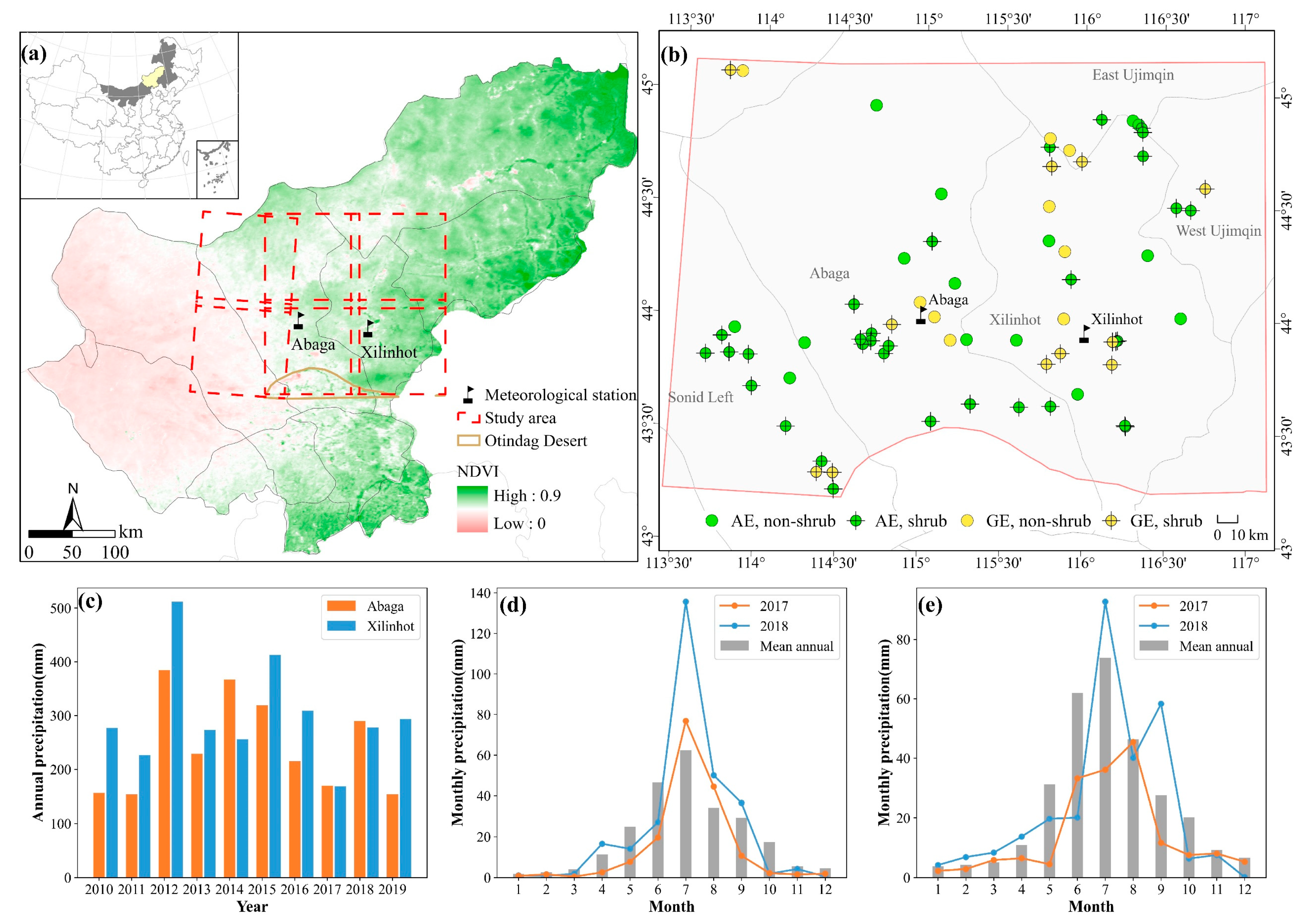
Figure 2.
Examples of the original AE and GE image (left), the object-oriented classification results (middle) and the shrub coverage with a resolution of 20 m (right). (a,b) are AE samples, and (c) is GE sample.
Figure 2.
Examples of the original AE and GE image (left), the object-oriented classification results (middle) and the shrub coverage with a resolution of 20 m (right). (a,b) are AE samples, and (c) is GE sample.
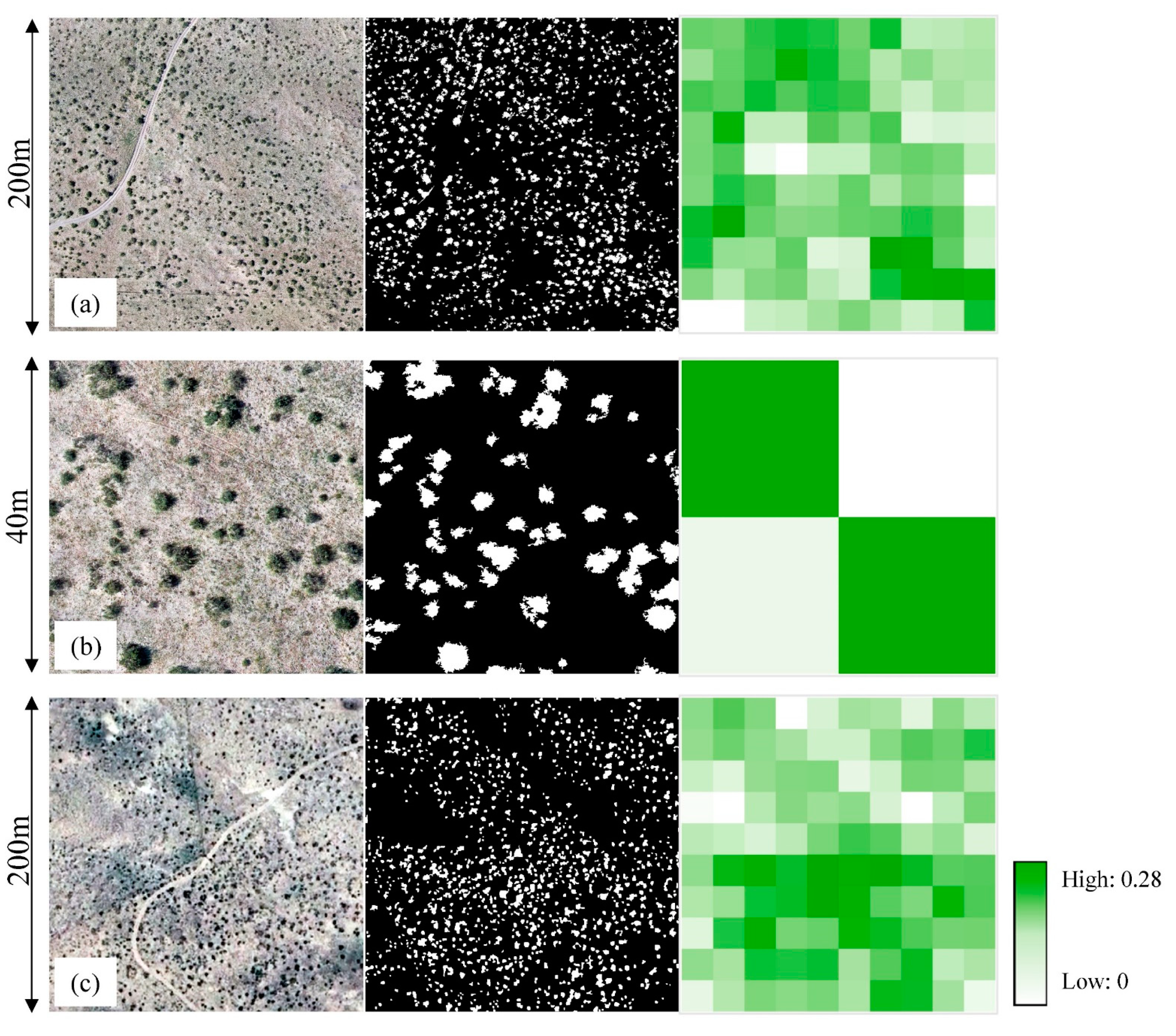
Figure 3.
Scatter plot of SSE and cluster numbers (k) of four sets of precipitation data (a), the spatial distribution of clustering results (b), and the multi-year averaged monthly precipitation of each subregion (c).
Figure 3.
Scatter plot of SSE and cluster numbers (k) of four sets of precipitation data (a), the spatial distribution of clustering results (b), and the multi-year averaged monthly precipitation of each subregion (c).
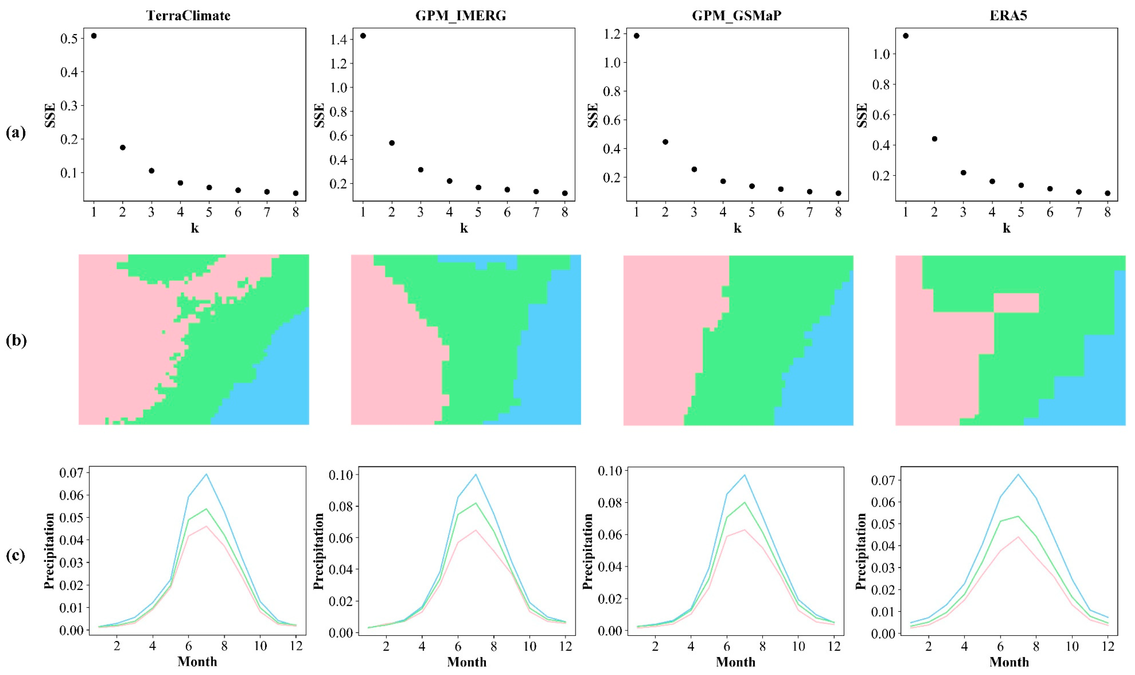
Figure 4.
The zoning results of the study area (a) and the violin histogram of shrub coverage for sample pixels in each subregion (b). The locations of training samples (green dots) and test samples (red dots) in each subregion are shown in (a). The number on (b) represents the total number of pixels in each subregion.
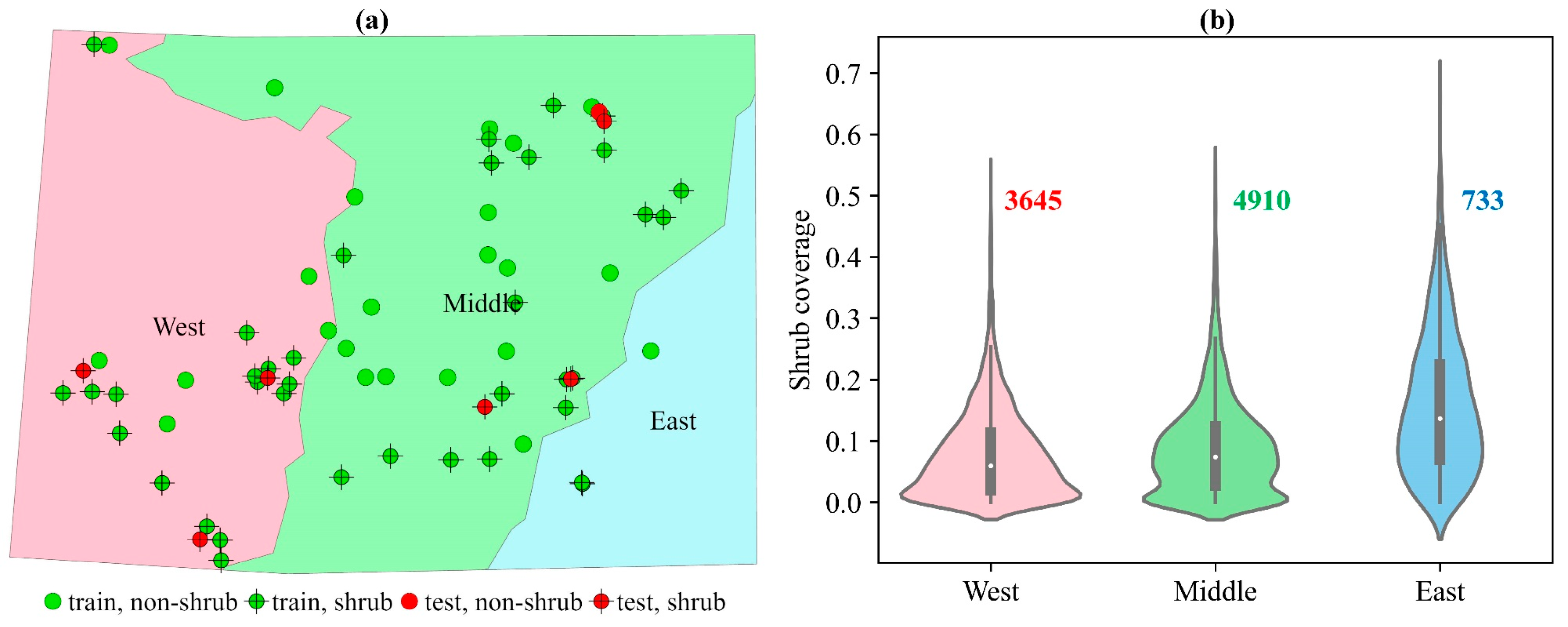
Figure 5.
Validation accuracy and test accuracy of RFR (a), SVR (b), PLSR (c), and GPR (d) methods in the West subregion. Diamonds are outliers beyond the upper and lower quartiles by 1.5 times the interquartile range.
Figure 5.
Validation accuracy and test accuracy of RFR (a), SVR (b), PLSR (c), and GPR (d) methods in the West subregion. Diamonds are outliers beyond the upper and lower quartiles by 1.5 times the interquartile range.
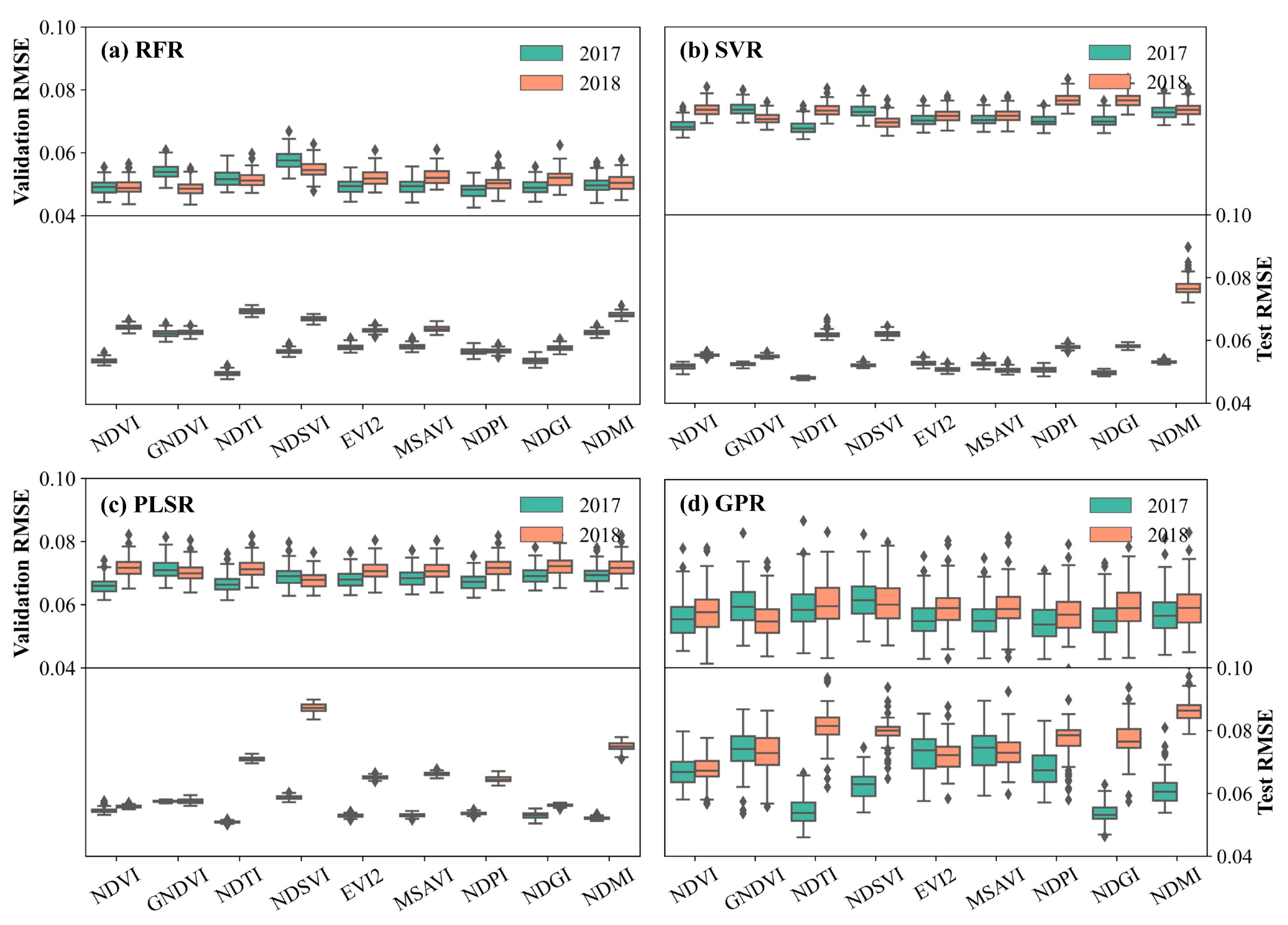
Figure 6.
Validation accuracy and test accuracy of RFR (a), SVR (b), PLSR (c), and GPR (d) methods in the Middle subregion. Diamonds are outliers beyond the upper and lower quartiles by 1.5 times the interquartile range.
Figure 6.
Validation accuracy and test accuracy of RFR (a), SVR (b), PLSR (c), and GPR (d) methods in the Middle subregion. Diamonds are outliers beyond the upper and lower quartiles by 1.5 times the interquartile range.

Figure 7.
Validation accuracy of RFR (a), SVR (b), PLSR (c), and GPR (d) methods in the East subregion. Diamonds are outliers beyond the upper and lower quartiles by 1.5 times the interquartile range.
Figure 7.
Validation accuracy of RFR (a), SVR (b), PLSR (c), and GPR (d) methods in the East subregion. Diamonds are outliers beyond the upper and lower quartiles by 1.5 times the interquartile range.
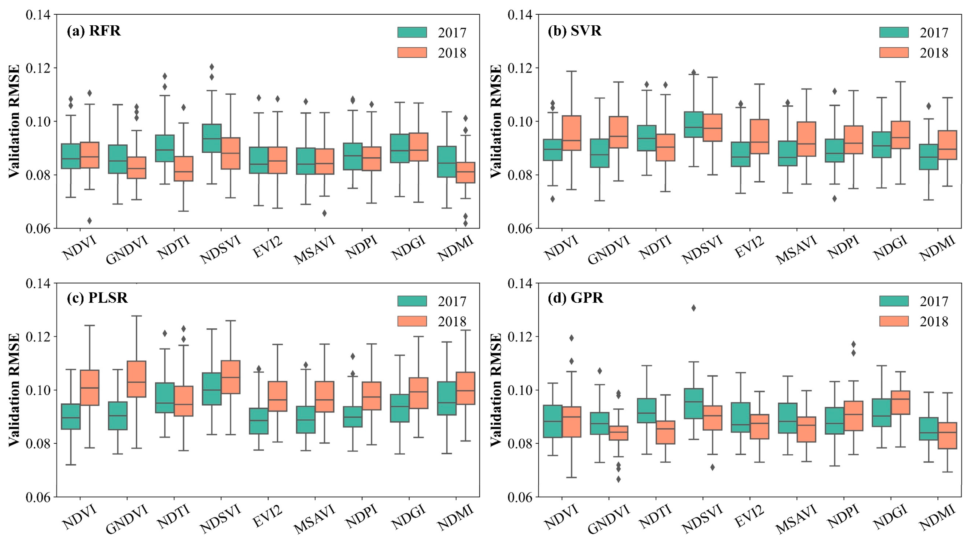
Figure 8.
Integrated ranking results of feature importance of RFR and GPR in 2017 (a–c) and 2018 (d–f). From blue to red, the climbing ranking values indicate the increase in feature importance.
Figure 8.
Integrated ranking results of feature importance of RFR and GPR in 2017 (a–c) and 2018 (d–f). From blue to red, the climbing ranking values indicate the increase in feature importance.

Figure 9.
The scatter plots of the true and predicted shrub coverage of the validation samples (a–d) and test samples (e–h) based on Stgy.1–4.
Figure 9.
The scatter plots of the true and predicted shrub coverage of the validation samples (a–d) and test samples (e–h) based on Stgy.1–4.

Figure 10.
The shrub coverage mapping result at 20 m resolution (upper), and the comparison of high spatial resolution images at locations A–E (middle row) and the predicted shrub coverage of the test samples at above locations (bottom row).
Figure 10.
The shrub coverage mapping result at 20 m resolution (upper), and the comparison of high spatial resolution images at locations A–E (middle row) and the predicted shrub coverage of the test samples at above locations (bottom row).

Figure 11.
The different growth status of Caragana shrubs in the West ((a), 43°50′N, 114°47′E) and Middle ((b), 44°31′N,116°34′E) subregions. Pictures were taken from the field UAV sampling experiment in August 2020.
Figure 11.
The different growth status of Caragana shrubs in the West ((a), 43°50′N, 114°47′E) and Middle ((b), 44°31′N,116°34′E) subregions. Pictures were taken from the field UAV sampling experiment in August 2020.
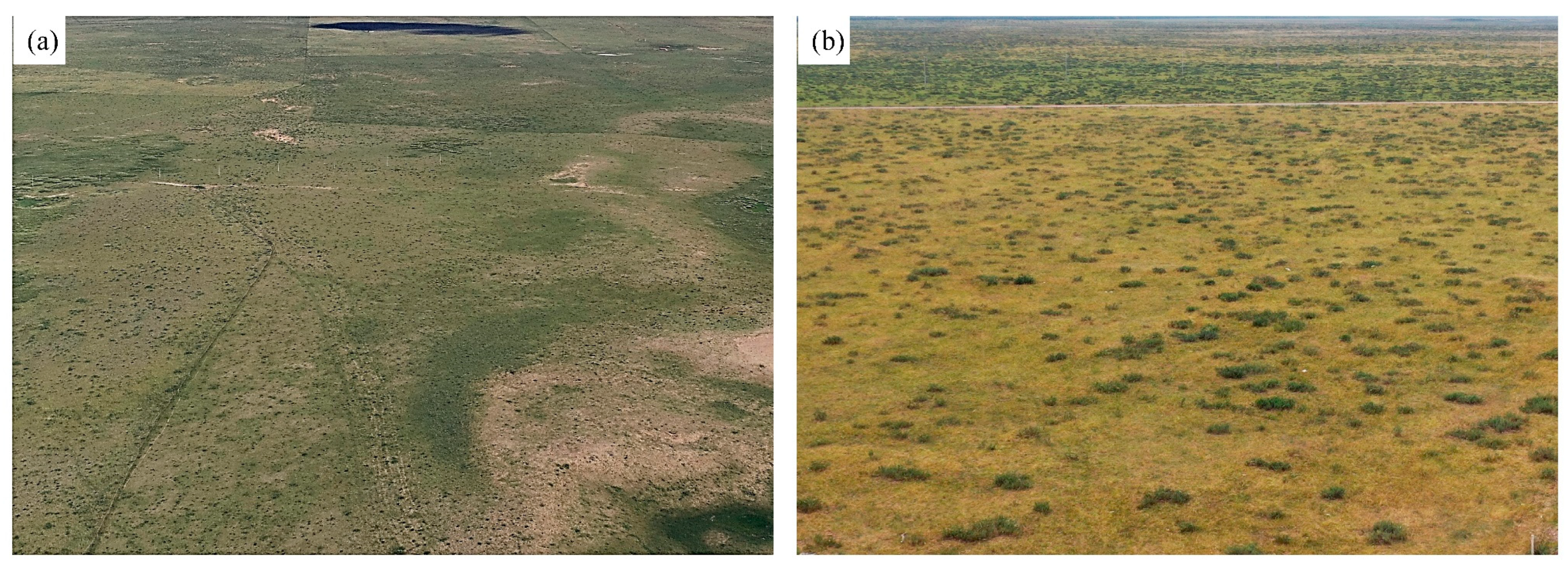
Figure 12.
The sensitivity of shrub monitoring accuracy to the temporal resolution of vegetation index time series. Dots and bars represent the mean and standard deviation of repeated cross-validation accuracy, respectively.
Figure 12.
The sensitivity of shrub monitoring accuracy to the temporal resolution of vegetation index time series. Dots and bars represent the mean and standard deviation of repeated cross-validation accuracy, respectively.

Table 1.
Attributes of precipitation reanalysis data.
| Name | Temporal Resolution | Spatial Resolution | Cover Time |
|---|---|---|---|
| TerraClimate | monthly | ~5 km | 1958–2019 |
| GPM_IMERG | 3 h | ~10 km | 2000–now |
| GPM_GSMap | hourly | ~10 km | 2000–now |
| ERA5 | hourly | ~25 km | 1979–now |
Table 2.
Selected vegetation indices for shrub coverage mapping.
| Type | Vegetation Index | Formula | Reference |
|---|---|---|---|
| Greenness Index | NDVI | [40] | |
| GNDVI | [41] | ||
| Yellowness Index | NDTI | [42] | |
| NDSVI | [43] | ||
| Background-adjusted Index | EVI2 | [44] | |
| MSAVI | [45] | ||
| NDPI | [46] | ||
| NDGI | [47] | ||
| Moisture Index | NDMI | [48] |
Table 3.
The adjustment range of regression methods’ parameters.
| Regression Methods | Parameter | Adjustment Range |
|---|---|---|
| RFR | max_features | 1, 2, 3, 4, 5, 6 |
| SVR | C | 0.1, 0.5, 1 |
| gamma | 0.001, 0.01, 0.05, 0.1 | |
| PLSR | n_components | 1, 2, 3, 4, 5, 6, 7, 8, 9, 10, 11, 12 |
| GPR | K(x1, x2) | Kernel’s hyperparameters were automatically optimized in model fitting |
Table 4.
The average of validation accuracy and test accuracy of four mapping strategies.
| Accuracy | Validation | Test | ||||||
|---|---|---|---|---|---|---|---|---|
| Stgy.1 | Stgy.2 | Stgy.3 | Stgy.4 | Stgy.1 | Stgy.2 | Stgy.3 | Stgy.4 | |
| RMSE | 0.050 | 0.050 | 0.050 | 0.050 | 0.052 | 0.055 | 0.057 | 0.060 |
| OA | 0.830 | 0.824 | 0.831 | 0.830 | 0.764 | 0.797 | 0.755 | 0.746 |
| Precision | 0.797 | 0.793 | 0.795 | 0.795 | 0.800 | 0.815 | 0.792 | 0.801 |
| Recall | 0.964 | 0.960 | 0.973 | 0.970 | 0.917 | 0.946 | 0.917 | 0.886 |
| Mean0 | 0.024 | 0.023 | 0.026 | 0.025 | 0.056 | 0.045 | 0.058 | 0.050 |
Note: Stgy.1 is zoning + full time series, Stgy.2 is zoning + key phenological period, Stgy.3 is non-zoning + full time series and Stgy.4 is non-zoning + key phenological period. The highest precision indicators for test accuracy are shown in bold.
Publisher’s Note: MDPI stays neutral with regard to jurisdictional claims in published maps and institutional affiliations. |
© 2022 by the authors. Licensee MDPI, Basel, Switzerland. This article is an open access article distributed under the terms and conditions of the Creative Commons Attribution (CC BY) license (https://creativecommons.org/licenses/by/4.0/).
Share and Cite
MDPI and ACS Style
Gan, L.; Cao, X.; Chen, X.; He, Q.; Cui, X.; Zhao, C. Mapping Shrub Coverage in Xilin Gol Grassland with Multi-Temporal Sentinel-2 Imagery. Remote Sens. 2022, 14, 3266. https://doi.org/10.3390/rs14143266
AMA Style
Gan L, Cao X, Chen X, He Q, Cui X, Zhao C. Mapping Shrub Coverage in Xilin Gol Grassland with Multi-Temporal Sentinel-2 Imagery. Remote Sensing. 2022; 14(14):3266. https://doi.org/10.3390/rs14143266
Chicago/Turabian StyleGan, Liqin, Xin Cao, Xuehong Chen, Qian He, Xihong Cui, and Chenchen Zhao. 2022. "Mapping Shrub Coverage in Xilin Gol Grassland with Multi-Temporal Sentinel-2 Imagery" Remote Sensing 14, no. 14: 3266. https://doi.org/10.3390/rs14143266
Note that from the first issue of 2016, this journal uses article numbers instead of page numbers. See further details here.