Abstract
The leaf area index (LAI) is critical for the respiration, transpiration, and photosynthesis of crops. Color indices (CIs) and vegetation indices (VIs) extracted from unmanned aerial vehicle (UAV) imagery have been widely applied to the monitoring of the crop LAI. However, when the coverage of the crop canopy is large and only spectral data are used to monitor the LAI of the crop, the LAI tends to be underestimated. The canopy height model (CHM) data obtained from UAV-based point clouds can represent the height and canopy structure of the plant. However, few studies have been conducted on the use of the CHM data in the LAI modelling. Thus, in this study, the feasibility of combining the CHM data and CIs and VIs, respectively, to establish LAI fitting models for winter wheat in four growth stages was investigated, and the impact of image resolution on the extraction of remote sensing variables (the CHM data, CIs, and VIs) and on the accuracy of the LAI models was evaluated. Experiments for acquiring remote sensing images of wheat canopies during the four growth stages from the RGB and multispectral sensors carried by a UAV were carried out. The partial least squares regression (PLSR), random forest regression (RFR), and support vector machine regression (SVR) were used to develop the LAI fitting models. Results showed that the accuracy of the wheat LAI models can be improved in the entire growth stages by the use of the additional CHM data with the increment of 0.020–0.268 in R2 for three regression methods. In addition, the improvement from the Cis-based models was more noticeable than the Vis-based ones. Furthermore, the higher the spatial resolution of the CHM data, the better the improvement made by the use of the additional CHM data. This result provides valuable insights and references for UAV-based LAI monitoring.
1. Introduction
The leaf area index (LAI), defined as the total one-sided leaf area per unit of the surface area of vegetation [], is a key parameter for the crop management and is closely related to photosynthesis, respiration, and transpiration of crop canopies [,]. The accurate and timely monitoring of the LAI is of great importance for efficient agricultural management []. Traditional methods for the monitoring of the LAI are expensive, laborious, and difficult to apply to the monitoring practice over large areas []. However, advances in remote sensing technologies may provide alternative methods for the monitoring of crop phenotypes in a cost-effective and timely manner at regional scales [,].
In previous studies, ground-based, airborne, and spaceborne platforms have been commonly used to obtain remote sensing data. Although data collected from ground-based sensors have high temporal and spatial resolutions, its disadvantages are high labor costs and limited coverage ranges []. In contrast, data from spaceborne platforms can cover wide spatial ranges and be obtained from multiple sources []. However, it is difficult for spaceborne platforms to acquire multi-temporal data of crops in a timely manner, due to the limitations of the fixed revisit cycle of the spaceborne platforms and weather influence []. The airborne platforms have gradually been employed in crop phenotypes monitoring for their high temporal resolution and flexible time selection of free flights [].
As one of the most commonly used airborne remote sensing platforms, an unmanned aerial vehicle (UAV) has recently been popularly used to collect images for crop growth monitoring [,]. Previous studies have shown that the spectral data obtained from RGB, multispectral, or hyperspectral sensors onboard UAVs can be used for the monitoring of crop phenotypes []. For example, color indices (CIs) derived from RGB imagery have been used for above-ground biomass estimation of maize []. Vegetation indices (VIs) extracted from the multispectral or hyperspectral sensors commonly contain the range of wavelengths that are strongly associated with crop growth (i.e., red edge (RE), near-infrared (NIR)) which have been widely applied in the monitoring of crop yields, LAI, ground biomass, and chlorophyll [,,]. However, CIs and VIs appear to be saturated in the case of a high proportion of soil background or excessive canopy biomass [].
According to [], for improving the accuracy of crop phenotypic monitoring, it is feasible to use the data from multiple sources and types, e.g., spectral, texture, and structure of canopies. Both canopy texture and spectral data generated from UAV-based RGB and multispectral imagery were used for the prediction of the LAI, above-ground biomass, and grain yields in [,]. The canopy structure data, e.g., a crop height model (CHM) collected from UAV-based point clouds, have been also applied in crop phenotypic monitoring. The CHM data were used, in addition to spectral data, in the monitoring of above-ground biomass and yield for a variety of crops [,,]. However, only a few studies examined the application of CHM data for the LAI monitoring [,], particularly using CHM data in the LAI modelling for the prediction of wheat LAI.
To fuse remote sensing data from various sensors for LAI fitting models, three machine learning algorithms—the partial least squares regression (PLSR), random forest regression (RFR), and support vector machine regression (SVR)—have been widely employed []. Since the PLSR method can deal with the multicollinearity among the model’s predictors, it was applied to the prediction for the LAI by Liu et al. [] and the results had good accuracy. Li et al. [] proved the effectiveness of using the RFR method to predict the LAI of crops, since this method has the advantage of expressing the nonlinear mappings between the feature of the remote sensing data and the phenotypes of the crop, and it is also not much affected by the noise and the number of the input variables []. SVR is the implementation of support vector machine for regression approximation, and has the ability to handle the data of high dimensionality and those less affected by sample size []. Therefore, both the PLSR, RFR, and SVR may be used to build LAI prediction models based on not only spectral data but also CHM data.
The main objectives of this study include: (1) to determine the quantitative relationship between the CHM data, CIs, VIs, and LAI of winter wheat during each stage of growth; (2) to investigate the potential of using the PLSR, RFR, and SVR methods and the sample data of both the CHM data and spectral data (i.e., the CIs and VIs) from UAV imagery to develop LAI fitting models for each stage of the growth; (3) to evaluate the effect of the spatial resolution of UAV imagery on the relationship between the LAI and the UAV-based remote sensing data (such as the CHM, CIs, and VIs) as well as on the LAI prediction.
2. Materials and Methods
2.1. Study Area
The location of the experimental site selected for this study is the experimental station of the Xuzhou Academy of Agricultural Sciences (XZAAS), in Xuzhou, Jiangsu province of China (117°23′48″E, 34°13′58″N, see Figure 1), where winter wheat (Xumai-33) is the predominant crop in the field, and the area studied was cultivated intensively. The fertilization method was the base fertilizer plus topdressing, with a base fertilizer dosage of 15,000 kg·ha−1 organic fertilizer, 450 kg·ha−1 NPK compound fertilizer (N:P:K = 15:15:15), and urea of 150 kg·ha−1, and a topdressing dosage urea of 225 kg·ha−1 in mid-March 2021. All LAI measurements were set up in a randomized block design, with 557 plots (each has a 1 m2 (1 m × 1 m) area) spanning four growth stages. The 63 and 27 LAI sampling plots of the maturation stage were coincident with those of the flowering and filling stage, respectively. The total area of LAI measurements is around 467 m2 in this study.
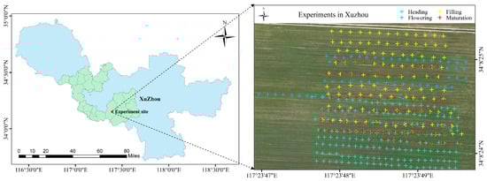
Figure 1.
Location of the experimental site (left) and the distribution of LAI measurements in the field (right) where different colors denote in different growth stages the LAI were measured.
2.2. Acquisition and Pre-Processing of Images
A DJI Phantom 4 multispectral version UAV (DJI-Innovations Inc., Shenzhen, China) was used to collect field images. It integrates one visible sensor and five single band sensors (Blue, Green, Red, RE, and NIR), and the specifications of these sensors are shown in Table 1. The UAV was flown in an automated mode and followed a pre-programmed flight plan to capture images with an approximately 75% front and a 60% side overlap during its flights. The images from the UAV had a resolution of 1600 × 1300 pixels at all four growth stages (Table 2), and the UAV flew at the three sensing heights of 50 m, 75 m, and 100 m, respectively, and their corresponding ground resolutions were 2.7 cm, 4.0 cm, 5.4 cm. The speed of the UAV was set to 5 m·s−1 and each flight was conducted from 11:00 am to 2:00 pm local time on sunny days with full sunlight and low wind speeds. Before each flight, the images of a calibration whiteboard with a 90% reflectance on the ground were collected to adjust the multispectral imagery for radiometric calibration with the empirical linear correction method. The DJI TERRA (DJI-Innovations Inc., Shenzhen, China) software was used to orthorectify and mosaic the images, and generate the digital surface model (DSM).

Table 1.
Specification of the multispectral image acquisition system used in this study.
Table 2.
Summary of field experiments conducted in 2021 during four stages of wheat growth.
2.3. Field Collection for LAI
Field LAI data (Table 2) were collected using a LAI-2200C (Li-Cor, Inc., Lincoln, NE, USA) at each sampling position including one reading above and eleven readings below the canopy. The LAI measurements were taken for 1–2 h between 4:00 pm to 7:30 pm local time, and four readings above the canopy (4A collections: diffuser caps in the sun, diffuser caps in the shadow, no cap in the shadow, and a normal reading) were conducted every 40 min. According to the instructions in the instrument documentation, the scattering corrections were conducted based on the 4A collections using LI-COR FV2200 software (v2.1) (Li-Cor, Inc., Lincoln, NE, USA) to compensate the bias caused by the change of light over time on LAI measurements. In addition, at the center of each plot, GPS data were recorded using a real-time kinematic global positioning system receiver for the identification of the position of the plot.
2.4. Image Processing and Data Extraction
2.4.1. CIs and VIs
The CIs and VIs are mathematical transformations of the spectra at the pre-defined wavelengths that are commonly employed to monitor crop growth parameters []. In this work, nine published VIs and seven CIs (see Table 3 for their formulas) were calculated for the modelling and predictions of the LAI, based on the studies [,]. The re-normalized r, g, and b bands were used to calculate the CIs from each sampling plot of RGB imagery [], as given by:
Table 3.
Formula for each of the CIs and VIs used in this study.
2.4.2. Extraction for CHM Data
The height of a crop is closely related to the growth of the crop []. A CHM, which is commonly calculated from UAV-based point clouds, can represent the canopy structure of the crop []. In recent years, CHM data together with spectral data were used to model and predict crop yields and above-ground biomass. In this study, the CHM data were obtained from a pixel-wise subtraction of the DSM and digital elevation model (DEM). The DSMs obtained from the UAV images during the bare soil period were treated as the DEM in the field, while the DSMs were obtained from the UAV images from each growth stage of winter wheat [,].
2.5. Data Analyses
2.5.1. Correlation Analysis
The relationship between the LAI measurements and the CHM data, CIs, and VIs extracted from UAV imageries at different flight altitudes was investigated using the Pearson correlation analysis expressed by (Equation (4)) below. The datasets for analyzing the effect of using both CHM data and spectral data on the LAI modelling result were determined based on the correlation calculated by:
where r is the correlation between the LAI measurement and the CHM data, CIs or VIs; i is the index of the sample; n is the number of the samples; x represents the CHM data, CIs or VIs; y is the LAI measurement.
2.5.2. Modeling Methods
In previous studies, machine learning methods have been widely applied in establishing the relationship between remote sensing data and crop parameters. In this study, three machine learning methods (PLSR, RFR, and SVR) were selected for wheat LAI fitting models constructing.
The PLSR, which integrates multiple linear regression, principal component analysis, and canonical correlation analysis, can address the problem of multicollinearity between a model’s predictors and be used to construct an accurate and stable linear model. The RFR introduces a random attribute selection in the training process of decision trees based on the bagging integration created by the decision trees. Specifically, the traditional decision tree selects the optimal attribute from the attribute set of the current node when the partition attribute is selected. However, in the RFR, for each node of the base decision tree, a subset containing k attributes is randomly selected from the attribute set of the node, and then the optimal attribute is identified from this subset. The RFR has the characteristics of randomly selecting branches on each decision tree node, which can simplify the correlation between the decision trees so that it can effectively deal with high-dimensional features. The number of trees (denoted by ntrees) is the most critical parameter of the RFR [] and when the value of ntrees is sufficiently large, it mostly influences the execution time rather than the modeling accuracy []. Thus, in this work, the value for ntrees was set to 500, which was the same as the value adopted in []. SVR is a significant application form of support vector machine, which has the less risk of over-fitting. The accuracy of the SVR models was mainly affected by model parameters. Thus, the radial basis kernel function (RBF) was selected as the kernel function, and the model parameter gamma (g) and regularization parameter (c) of the SVR method were estimated on training dataset using a grid search method with five-fold cross-validation in this study.
2.5.3. Accuracy Assessment
For the construction of the wheat LAI fitting models for this study, both PLSR, RFR, and SVR models were adopted and various combinations of input variable data, including CHM, CIs, CIs + CHM, VIs, and VIs + CHM, which were used as the sample data of the modelling. Two-thirds of the input data and LAI measurements were randomly selected for training samples, and the remaining data were treated as out-of-samples data to be used for the testing of the established fitting model. The coefficient of determination (R2, in Equation (5)) and the root mean square error (RMSE, in Equation (6)) were used to assess the effectiveness or accuracy of the LAI results predicted by the fitting models.
where and are the ith observed and predicted LAI values, respectively; is the mean of the observed LAI values; n is the number of the samples.
3. Results
3.1. Data Range of Wheat LAI
Table 4 shows the fundamental statistics of the LAI values from the training and testing datasets during each growth stage. For the training dataset, the data ranges of the LAI values during the heading, flowering, filling, maturation and entire growth period were 2.22−7.37 (CV = 24.91%), 1.84−5.45 (CV = 24.26%), 1.43−6.20 (CV = 33.05%), 1.71−4.97 (CV = 24.67%) and 1.43−7.37 (CV = 29.38%), respectively. The analysis of the data from the training dataset of different growth stages showed that the variation in the LAI values was larger in the filling and entire growth period than the other growth stages. The testing datasets in different stages have the similar features or distributions. Hence, the selection of the training and testing datasets for the LAI modelling is reasonable.
Table 4.
Data range of the LAI values from the training and testing datasets in each wheat growth stage.
3.2. Data Size Per Hectare
According to [], the digitization footprint contributions ascribable to UAV imagery and the CHM data were shown in Table 5. In this study, the required storage disc size per hectare of three types of data increased with the increased in spatial resolution. Additionally, at the same spatial resolution, the required data storage disc size for multispectral UAV imagery was significantly higher than that of the CHM data and RGB imagery.
Table 5.
Data size per hectare from three types of data at three flight altitudes.
3.3. Correlation between LAI and CHM Data, CIs and VIs
Figure 2 shows the correlation coefficient between the wheat LAI and the UAV-based CHM data, CIs, and VIs at each of the flight altitudes in each of the growth stages (heading, flowering, filling, maturation), respectively, and also the entire growth period. From the most left column, which is for the CHM results, comparing the three values in the same growth stage, we can find that the value at the 50 m altitude was the largest, followed by the 75 m altitude, and the weakest correlation was found at the 100 m altitude. Moreover, if the CHM results from the five different stages were compared, the largest correlation was in the heading stage (top), with the values of 0.80, 0.75, and 0.75 at the 50 m, 75 m, and 100 m altitudes, respectively. These results reveal the potential of using the CHM data in the modelling of the wheat LAI, which is for the prediction of the wheat LAI.
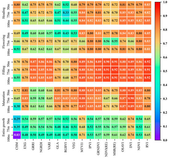
Figure 2.
Coefficient of Pearson’s correlation (r) between the LAI and the CHM data, CIs, and VIs in each growth stage at each altitude of the UAV observations.
From the second (EXG) to the eighth columns (VEG) in Figure 2 are the correlation results of the seven CIs. We can find that the correlation values of all these CIs in the heading stage from the same height were smaller than that of CHM, and it is also the same at the 50 m height in the flowering stage. However, in the remaining results, most of the correlation values of the CIs were larger than that of CHM. In addition, from the ninth to the last columns are the results of the nine VIs. The majority of their values were larger than that of the CIs, and they were less affected by flight altitudes. The DVI (the third last column) and RVI (the last column) presented the strongest correlations, compared to the other VIs in all five stages.
According to the above results, the CHM data, CIs, and VIs extracted from the UAV imagery at 50 m flight altitude were selected in Section 3.3 and Section 3.4 to analyze the effect of using the CHM data and spectral data for the wheat LAI models developed using the PLSR, RFR, and SVR methods.
3.4. LAI Prediction Accuracy from PLSR, RFR, and SVR over the Entire Growth Period
In this section, the following five combinations of data were used as the input data of the LAI fitting models developed using the PLSR, RFR, and SVR methods over the entire growth period: (1) CHM, (2) CIs, (3) CIs + CHM, (4) VIs, and (5) VIs + CHM. The PLSR, RFR, and SVR fitting models were tested using an out-of-sample dataset (i.e., the test data were not used in the modelling) and the results are shown in Table 6.
Table 6.
Accuracy of LAI predicted by the LAI models developed using the PLSR, RFR, and SVR, and five types of input datasets at the 50 m altitude in the entire growth period.
When using the CHM data alone, SVR achieved the best LAI prediction performance (R2 = 0.147, RMSE = 0.926) among the three regression methods. When using the CIs or VIs as the model input set, the best performance was also found for the SVR method. Moreover, the accuracy of VIs results was obviously better than that of CHM and CIs cases.
The combination of CHM and CIs led to obvious improvements for all regression methods than the CIs-only cases, with the increment of 0.158, 0.268 and 0.201 in R2 for PLSR, RFR, SVR, respectively. In addition, SVR achieved the highest accuracy (R2 = 0.652, RMSE = 0.591) in the LAI prediction. For VIs, the additional CHM data also enhanced the accuracy of the LAI models, with the increment of 0.046, 0.073 and 0.020 in R2 for PLSR, RFR, SVR, respectively.
Figure 3u–y shows the scatter plots for measured versus predicted LAI from optimal LAI fitting models in the entire growth period. It could be found that the combination of the CHM and spectral data led to the data points closer to the 1:1 line than the cases of using the CHM or spectral data only.
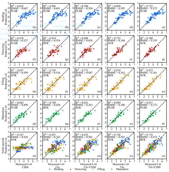
Figure 3.
Scatter plots for measured versus predicted LAI from optimal LAI fitting models from five types of input data in the heading (a–e), flowering (f–j), filling (k–o), maturation (p–t) and entire growth period (u–y), and the test data were independent of the sample data used in the modelling process (i.e., out-of-sample data).
3.5. LAI Prediction Accuracy for Individual Growth Stages
As shown in Figure 4, the performance of LAI fitting models was inconsistent across four individual growth stages for five types of input sets with three regression methods. In the cases of using the CHM data, CIs and the combination of the CHM data and CIs, the LAI prediction accuracy showed a trend of first decreasing and then increasing from the heading stage to the maturation stage. The increase in LAI prediction accuracy from the flowering to the filling stage was the most significant change in all adjacent stages. In addition, all three regression methods had the stable performance in the filling and the maturation stage. In contrary to the LAI prediction results of the entire growth period, using the CHM data as the model input set had the better performance in LAI prediction than that of the CIs in the heading and the flowering stages for SVR an PLSR methods. However, the combination of CHM and CIs led to a significant improvement in its resultant LAI, compared with the case of using the CHM data or CIs only in four individual growth stages.
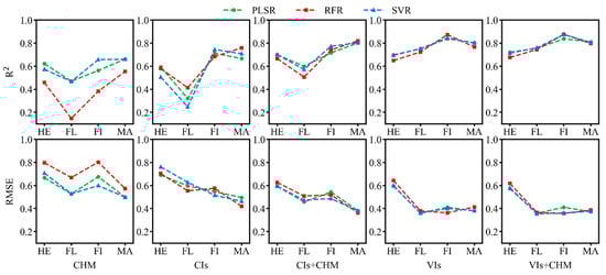
Figure 4.
The performance of LAI fitting models from five types of input data for four individual growth stages (HE: the heading stage; FL: the flowering stage; FI: the filling stage; MA: the maturation stage) with three regression methods.
When using VIs and VIs + CHM as the model input sets, the accuracy of the LAI fitting models showed an upward trend from the heading to the filling stage and decreased slightly in the maturation stage. All three regression methods had the stable performance in LAI prediction in four individual stages.
3.6. Effect of Spatial Resolution on LAI Prediction
In this study, the CIs and VIs extracted from UAV imagery at different altitudes in the heading, flowering, filling, and maturation stages had the pixel resolutions of 2.7 cm (50 m), 4.0 cm (75 m), and 5.4 cm (100 m), respectively; the pixel resolutions of the CHM data extracted were 5.4 cm (50 m), 8.0 cm (75 m), and 10.8 cm (100 m). The LAI fitting models based on the PLSR, RFR, and SVR methods, and the sample data of the CHM data, CIs and VIs extracted at the same flight altitudes were constructed, and their test results, i.e., the R2 and RMSE of the LAI values predicted by the models are shown in Figure 5.
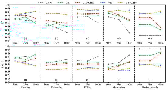
Figure 5.
R2 (a–e) and RMSE (f–j) of LAI values predicted by the optimal LAI fitting models resulting from five types of input datasets at each altitude in each growth stage.
For using the CHM data only, the accuracy of the LAI prediction increased with the increased in spatial resolution in each individual growth stage. However, as shown in Figure 5e,j, the increase in spatial resolution of the CHM data had no significant impact on LAI prediction in the entire growth period.
From the R2 and RMSE results of the CIs-only case (green in each pane) in the heading, flowering and entire growth period, one can see that the highest accuracy of the LAI prediction was at the 75 m altitude, followed by 50 m and 100 m; while in the other two stages, the accuracy of the LAI prediction decreased with the decrease in spatial resolution. Moreover, the accuracy of the CIs + CHM results in each growth stage was obviously improved for all flight altitudes compared with the results of the CIs-only case, meaning the contribution made by the use of the CHM data in the LAI modeling based on RGB imagery.
For the VIs-only case, the accuracy of the LAI prediction at the 100 m altitude was significantly better than the 50 m and 75 m altitudes; and only in the flowering stage the highest accuracy of the LAI prediction was at the 75 m altitude, followed by 50 m and 100 m. Moreover, the CHM + VIs results significantly improved only in the heading stage and the entire growth period. However, in the rest three stages the introduction of the CHM data did not improve the accuracy.
4. Discussion
4.1. Using CHM Data Combined with Either CIs or VIs in LAI Modelling
The CHM data, CIs, and VIs selected for this study were extracted from the orthophoto images obtained by a DJI Innovations 4 multispectral version UAV, which was equipped with visible and multispectral sensors. The scatter plots of the optimal LAI fitting models resulting from the five types of input sets extracted from the UAV imagery at the 50 m flight altitude are shown in Figure 3.
The canopy height is an important parameter of crop vertical structure []. The CHM data, which are commonly calculated from a pixel-wise subtraction of the DSM and DEM, have been proved to have a moderate relationship with the crop LAI []. This was confirmed by the good performance of using the CHM data for wheat LAI prediction in four individual growth stages in this study. However, the use of the CHM data only was insufficient for the LAI prediction in the entire period (Figure 3u) and the LAI prediction accuracy of the model with CHM data as the input set was significantly lower than that of individual growth stages. This is likely due to the fact that height of the winter wheat does not change significantly from the flowering to maturation stage [], but the LAI of the winter wheat decreases after the heading stage.
In recent years, CIs extracted from UAV-based RGB imagery are widely used in the field of precision agriculture [,]. From the second left column in Figure 3, which displays the Cis results, we can find that the Cis could be used to obtain the wheat LAI in the filling (Figure 3l) and maturation (Figure 3q) stages. However, the use of CIs only is insufficient for the LAI prediction in the heading (Figure 3b), flowering (Figure 3g) and entire growth period (Figure 3v), which is consistent wduction ith the research []. However, as shown in the middle column, the CIs + CHM results led to significant improvements in the accuracy of the LAI prediction in all five stages, which mainly reflected in the improvement of the underestimation of the LAI when LAI values are high. This finding is consistent with [], which stated that the fusion of CIs and canopy height obtained from a low-cost UAV system can improve the prediction of wheat above-ground biomass.
The accuracy of the LAI values predicted by the models resulting from the VIs-only case (the second right column) were better than that of the CIs cases. This is mainly because the VIs calculated based on RE and NIR (i.e., NDVIRE, MSRRE) reflect the crop growing process better than the CIs []. It is worth nothing that the results from the use of CIs + CHM in the heading (Figure 3c) and maturation stages (Figure 3r) were similar to that of the VIs cases, which demonstrates the potential of combining spectral data of RGB images with CHM data in wheat LAI monitoring.
From the last column (the case of VIs + CHM), one can find that the use of the CHM data in addition to the VIs enhanced the accuracy of the LAI models, and the improvement made by the CHM was also reflected in the amelioration of underprediction of the LAI with high values, which was similar to the improvement made by the adding of the CHM data to the CIs-based models. Similar findings were also reported by Gong et al. [], who found the model based on the VIs and canopy height mitigated the hysteresis effect caused by phenology differences, which significantly enhanced the accuracy of the rice LAI prediction throughout the growing season. However, as shown in Figure 2 and Figure 3, the CHM data extracted from the 50 m flight altitude showed strong correlations with the wheat LAI in each single stage, but the accuracy of the LAI prediction from CHM + VIs was slightly better than that of using the VIs only in the same stage. This is likely due to the stronger correlations between the VIs and the LAI than the correlation between the CHM data and the LAI in each single stage.
4.2. The Optimal Spatial Resolution of the CHM data for LAI Prediction
The resolution of remote sensing data is considered to be an important factor for the accuracy of the LAI prediction of crops []. As shown in Figure 5, the optimal image resolution for LAI prediction was different for different types of remote sensing variables. Thus, the CHM data and the spectral data obtained at different flight altitudes (50 m, 75 m, and 100 m) were combined as the input set of the PLSR, RFR, and SVR methods, and their test results are shown in Figure 6 and Figure 7.
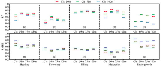
Figure 6.
R2 (a–e) and RMSE (f–j) of LAI values predicted by the optimal LAI fitting models resulting from the combination of CIs and the CHM data from 50 m, 75 m and 100 m flight altitude in each growth stage, respectively. The x axis number represents the combination of the CIs and CHM data obtained at the different flight altitudes.
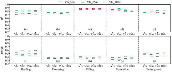
Figure 7.
R2 (a–e) and RMSE (f–j) of LAI values predicted by the optimal LAI fitting models resulting from the combination VIs and the CHM data from 50 m, 75 m and 100 m flight altitude in each growth stage, respectively. The x axis number represents the combination of the CIs and CHM data obtained at the different flight altitudes.
Figure 6 shows the LAI prediction results of models with the combination of CIs and the CHM data as the input set, it could be found that the use of additional CHM data obtained at different flight altitude can improve the accuracy of CIs-based models. In addition, the accuracy of the LAI fitting models increased with the increase in spatial resolution of the CHM data in most cases.
For VIs-based cases (see Figure 7), the combination of the VIs from 50 m altitude and CHM data enhanced the accuracy of the LAI models only in the heading and entire growth period. However, the model accuracy decreased due to additional the CHM data obtained at 75 m and 100 m in the flowering and maturation stages. When the CHM data of different resolutions were combined with the VIs acquired at the flight altitude of 75 m as the input set, only the use of the CHM data obtained from 50 m flight altitude in addition to the VIs improved the model accuracy obviously in all stages. For the cases of VIs from 100 m altitude, only the additional CHM data from 50 m significantly improved the VIs-based models in the heading, maturation, and entire growth period.
According to the above results, in most cases, the effect of additional CHM data on improving the accuracy of CIs-only model was increased with the improvement of spatial resolution of the CHM data. However, for the cases of using VIs and the CHM data as the input sets, only the CHM data obtained at 50 m flight altitude had more stable and excellent contributions for VIs-only model in each growth period.
5. Conclusions
This study investigated the potential of combining the CHM and spectral data (CIs, VIs) obtained from a low-altitude UAV in wheat LAI modeling based on PLSR, RFR, and SVR methods. The results demonstrated that the accuracy of the CIs-based LAI prediction models was obviously improved by the use of the additional CHM data. For the VIs case, the improvement of the CHM data for a better LAI prediction was mainly reflected in the heading and entire growth period but was not significant in the other three stages. Moreover, the performance of the CHM data, CIs, and VIs under different image resolutions was analyzed, and the results showed the additional CHM data at the resolution of 5.4 cm had the best performance in improving the LAI prediction accuracy.
The results from this study suggest the effectiveness the combination of the CHM data and CIs in the wheat LAI modelling in and after the heading stage for the wheat LAI monitoring. However, for the LAI monitoring based on multispectral UAV imagery, only the CHM data with high spatial resolution may improve the LAI prediction accuracy more obviously in heading and entire growth period. Our future work will be focused on more investigations on the influence of using the CHM data on the wheat LAI model results before the heading stage, and on the contribution of using the CHM data from different types of crops in each growth stage.
Author Contributions
Conceptualization, X.Z. and K.Z.; methodology, X.Z. and C.B.; software, X.Z. and S.C.; validation, X.Z. and Y.S.; formal analysis, X.Z. and W.B.; investigation, X.Z., Y.Z. and H.S.; resources, X.Z., E.F. and H.S.; data curation, X.Z., C.B. and S.C.; writing—original draft preparation, X.Z. and K.Z.; writing—review and editing, X.Z., H.S., S.W. and K.Z.; visualization, X.Z.; supervision, S.W. and K.Z.; project administration, K.Z. and Y.S.; funding acquisition, K.Z., Y.S. and H.S. All authors have read and agreed to the published version of the manuscript.
Funding
This work was funded in part by the National Natural Science Foundation of China under Grant No. 42274021, in part by 2022 Jiangsu Provincial Science and Technology Initiative—Special Fund for International Science and Technology Cooperation under Grant No. BZ2022018, in part by Key Laboratory of National Geographic Census and Monitoring, Ministry of Natural Resources under Grant No. 2022NGCM04, in part by Natural Science Foundation of Jiangsu Province under Grant No. BK20190644, and in part by the Xuzhou Key R&D Program under Grant No. KC19111 and Grant No. KC20181.
Data Availability Statement
Not applicable.
Conflicts of Interest
The authors declare no conflict of interest.
References
- Watson, D.J. Comparative Physiological Studies on the Growth of Field Crops: II. The Effect of Varying Nutrient Supply on Net Assimilation Rate and Leaf Area. Ann. Bot. 1947, 11, 375–407. [Google Scholar] [CrossRef]
- Qu, Y.H.; Wang, Z.X.; Shang, J.L.; Liu, J.G.; Zou, J. Estimation of leaf area index using inclined smartphone camera. Comput. Electron. Agric. 2021, 191, 106514. [Google Scholar] [CrossRef]
- Yan, G.J.; Hu, R.H.; Luo, J.H.; Weiss, M.; Jiang, H.L.; Mu, X.H.; Xie, D.H.; Zhang, W.M. Review of indirect optical measurements of leaf area index: Recent advances, challenges, and perspectives. Agric. For. Meteorol. 2019, 265, 390–411. [Google Scholar] [CrossRef]
- Lan, Y.B.; Huang, Z.X.; Deng, X.L.; Zhu, Z.H.; Huang, H.S.; Zheng, Z.; Lian, B.Z.; Zeng, G.L.; Tong, Z.J. Comparison of machine learning methods for citrus greening detection on UAV multispectral images. Comput. Electron. Agric. 2020, 171, 105234. [Google Scholar] [CrossRef]
- Behera, S.K.; Srivastava, P.; Pathre, U.V.; Tuli, R. An indirect method of estimating leaf area index in Jatropha curcas L. using LAI-2000 Plant Canopy Analyzer. Agric. For. Meteorol. 2010, 150, 307–311. [Google Scholar] [CrossRef]
- dela Torre, D.M.G.; Gao, J.; Macinnis-Ng, C. Remote sensing-based estimation of rice yields using various models: A critical review. Geo-Spat. Inf. Sci. 2021, 24, 580–603. [Google Scholar] [CrossRef]
- Jonckheere, I.; Fleck, S.; Nackaerts, K.; Muys, B.; Coppin, P.; Weiss, M.; Baret, F. Review of methods for in situ leaf area index determination. Agric. For. Meteorol. 2004, 121, 19–35. [Google Scholar] [CrossRef]
- Zheng, H.; Cheng, T.; Li, D.; Yao, X.; Tian, Y.; Cao, W.; Zhu, Y. Combining Unmanned Aerial Vehicle (UAV)-Based Multispectral Imagery and Ground-Based Hyperspectral Data for Plant Nitrogen Concentration Estimation in Rice. Front Plant Sci 2018, 9, 936. [Google Scholar] [CrossRef]
- Yu, L.; Shang, J.; Cheng, Z.; Gao, Z.; Wang, Z.; Tian, L.; Wang, D.; Che, T.; Jin, R.; Liu, J.; et al. Assessment of Cornfield LAI Retrieved from Multi-Source Satellite Data Using Continuous Field LAI Measurements Based on a Wireless Sensor Network. Remote Sens. 2020, 12, 3304. [Google Scholar] [CrossRef]
- Liu, S.; Jin, X.; Nie, C.; Wang, S.; Yu, X.; Cheng, M.; Shao, M.; Wang, Z.; Tuohuti, N.; Bai, Y.; et al. Estimating leaf area index using unmanned aerial vehicle data: Shallow vs. deep machine learning algorithms. Plant Physiol. 2021, 187, 1551–1576. [Google Scholar] [CrossRef] [PubMed]
- Arroyo-Mora, J.P.; Kalacska, M.; Loke, T.; Schlapfer, D.; Coops, N.C.; Lucanus, O.; Leblanc, G. Assessing the impact of illumination on UAV pushbroom hyperspectral imagery collected under various cloud cover conditions. Remote Sens. Environ. 2021, 258, 112396. [Google Scholar] [CrossRef]
- Xu, W.C.; Yang, W.G.; Chen, S.D.; Wu, C.S.; Chen, P.C.; Lan, Y.B. Establishing a model to predict the single boll weight of cotton in northern Xinjiang by using high resolution UAV remote sensing data. Comput. Electron. Agric. 2020, 179, 105762. [Google Scholar] [CrossRef]
- Tetila, E.C.; Machado, B.B.; Menezes, G.K.; Oliveira, A.D.; Alvarez, M.; Amorim, W.P.; Belete, N.A.D.; da Silva, G.G.; Pistori, H. Automatic Recognition of Soybean Leaf Diseases Using UAV Images and Deep Convolutional Neural Networks. IEEE Geosci. Remote Sens. Lett. 2020, 17, 903–907. [Google Scholar] [CrossRef]
- Maes, W.H.; Steppe, K. Perspectives for Remote Sensing with Unmanned Aerial Vehicles in Precision Agriculture. Trends Plant Sci. 2019, 24, 152–164. [Google Scholar] [CrossRef]
- Niu, Y.X.; Zhang, L.Y.; Zhang, H.H.; Han, W.T.; Peng, X.S. Estimating Above-Ground Biomass of Maize Using Features Derived from UAV-Based RGB Imagery. Remote Sens. 2019, 11, 1261. [Google Scholar] [CrossRef]
- Cao, Y.; Li, G.L.; Luo, Y.K.; Pan, Q.; Zhang, S.Y. Monitoring of sugar beet growth indicators using wide-dynamic-range vegetation index (WDRVI) derived from UAV multispectral images. Comput. Electron. Agric. 2020, 171, 105331. [Google Scholar] [CrossRef]
- Wang, F.M.; Yi, Q.X.; Hu, J.H.; Xie, L.L.; Yao, X.P.; Xu, T.Y.; Zheng, J.Y. Combining spectral and textural information in UAV hyperspectral images to estimate rice grain yield. Int. J. Appl. Earth Obs. Geoinf. 2021, 102, 102397. [Google Scholar] [CrossRef]
- Feng, L.; Chen, S.S.; Zhang, C.; Zhang, Y.C.; He, Y. A comprehensive review on recent applications of unmanned aerial vehicle remote sensing with various sensors for high-throughput plant phenotyping. Comput. Electron. Agric. 2021, 182, 106033. [Google Scholar] [CrossRef]
- Zheng, H.B.; Cheng, T.; Zhou, M.; Li, D.; Yao, X.; Tian, Y.C.; Cao, W.X.; Zhu, Y. Improved estimation of rice aboveground biomass combining textural and spectral analysis of UAV imagery. Precis. Agric. 2019, 20, 611–629. [Google Scholar] [CrossRef]
- Maimaitijiang, M.; Sagan, V.; Sidike, P.; Hartling, S.; Esposito, F.; Fritschi, F.B. Soybean yield prediction from UAV using multimodal data fusion and deep learning. Remote Sens. Environ. 2020, 237, 111599. [Google Scholar] [CrossRef]
- Bendig, J.; Yu, K.; Aasen, H.; Bolten, A.; Bennertz, S.; Broscheit, J.; Gnyp, M.L.; Bareth, G. Combining UAV-based plant height from crop surface models, visible, and near infrared vegetation indices for biomass monitoring in barley. Int. J. Appl. Earth Obs. Geoinf. 2015, 39, 79–87. [Google Scholar] [CrossRef]
- Li, B.; Xu, X.M.; Zhang, L.; Han, J.W.; Bian, C.S.; Li, G.C.; Liu, J.G.; Jin, L.P. Above-ground biomass estimation and yield prediction in potato by using UAV-based RGB and hyperspectral imaging. ISPRS J. Photogramm. Remote Sens. 2020, 162, 161–172. [Google Scholar] [CrossRef]
- Li, W.; Niu, Z.; Chen, H.Y.; Li, D.; Wu, M.Q.; Zhao, W. Remote estimation of canopy height and aboveground biomass of maize using high-resolution stereo images from a low-cost unmanned aerial vehicle system. Ecol. Indic. 2016, 67, 637–648. [Google Scholar] [CrossRef]
- Peprah, C.O.; Yamashita, M.; Yamaguchi, T.; Sekino, R.; Takano, K.; Katsura, K. Spatio-Temporal Estimation of Biomass Growth in Rice Using Canopy Surface Model from Unmanned Aerial Vehicle Images. Remote Sens. 2021, 13, 2388. [Google Scholar] [CrossRef]
- Maimaitijiang, M.; Ghulam, A.; Sidike, P.; Hartling, S.; Maimaitiyiming, M.; Peterson, K.; Shavers, E.; Fishman, J.; Peterson, J.; Kadam, S.; et al. Unmanned Aerial System (UAS)-based phenotyping of soybean using multi-sensor data fusion and extreme learning machine. ISPRS J. Photogramm. Remote Sens. 2017, 134, 43–58. [Google Scholar] [CrossRef]
- Reisi Gahrouei, O.; McNairn, H.; Hosseini, M.; Homayouni, S. Estimation of Crop Biomass and Leaf Area Index from Multitemporal and Multispectral Imagery Using Machine Learning Approaches. Can. J. Remote Sens. 2020, 46, 84–99. [Google Scholar] [CrossRef]
- Li, S.Y.; Yuan, F.; Ata-UI-Karim, S.T.; Zheng, H.B.; Cheng, T.; Liu, X.J.; Tian, Y.C.; Zhu, Y.; Cao, W.X.; Cao, Q. Combining Color Indices and Textures of UAV-Based Digital Imagery for Rice LAI Estimation. Remote Sens. 2019, 11, 1763. [Google Scholar] [CrossRef]
- Wang, L.A.; Zhou, X.D.; Zhu, X.K.; Dong, Z.D.; Guo, W.S. Estimation of biomass in wheat using random forest regression algorithm and remote sensing data. Crop J. 2016, 4, 212–219. [Google Scholar] [CrossRef]
- Maimaitijiang, M.; Sagan, V.; Sidike, P.; Daloye, A.M.; Erkbol, H.; Fritschi, F.B. Crop Monitoring Using Satellite/UAV Data Fusion and Machine Learning. Remote Sens. 2020, 12, 1357. [Google Scholar] [CrossRef]
- Dong, T.F.; Liu, J.G.; Shang, J.L.; Qian, B.D.; Ma, B.L.; Kovacs, J.M.; Walters, D.; Jiao, X.F.; Geng, X.Y.; Shi, Y.C. Assessment of red-edge vegetation indices for crop leaf area index estimation. Remote Sens. Environ. 2019, 222, 133–143. [Google Scholar] [CrossRef]
- Meyer, G.E.; Neto, J.C. Verification of color vegetation indices for automated crop imaging applications. Comput. Electron. Agric. 2008, 63, 282–293. [Google Scholar] [CrossRef]
- Woebbecke, D.M.; Meyer, G.E.; Bargen, K.V.; Mortensen, D.A. Color Indices for Weed Identification Under Various Soil, Residue, and Lighting Conditions. Trans. ASAE 1995, 38, 259–269. [Google Scholar] [CrossRef]
- Verrelst, J.; Schaepman, M.E.; Koetz, B.; Kneubuhler, M. Angular sensitivity analysis of vegetation indices derived from CHRIS/PROBA data. Remote Sens. Environ. 2008, 112, 2341–2353. [Google Scholar] [CrossRef]
- Tucker, C.J. Red and photographic infrared linear combinations for monitoring vegetation. Remote Sens. Environ. 1979, 8, 127–150. [Google Scholar] [CrossRef]
- Gitelson, A.A.; Kaufman, Y.J.; Stark, R.; Rundquist, D. Novel algorithms for remote estimation of vegetation fraction. Remote Sens. Environ. 2002, 80, 76–87. [Google Scholar] [CrossRef]
- Louhaichi, M.; Borman, M.M.; Johnson, D.E. Spatially Located Platform and Aerial Photography for Documentation of Grazing Impacts on Wheat. Geocarto Int. 2008, 16, 65–70. [Google Scholar] [CrossRef]
- Hague, T.; Tillett, N.D.; Wheeler, H. Automated crop and weed monitoring in widely spaced cereals. Precis. Agric. 2006, 7, 21–32. [Google Scholar] [CrossRef]
- Becker, F.; Choudhury, B.J. Relative sensitivity of normalized difference vegetation Index (NDVI) and microwave polarization difference Index (MPDI) for vegetation and desertification monitoring. Remote Sens. Environ. 1988, 24, 297–311. [Google Scholar] [CrossRef]
- Gitelson, A.; Merzlyak, M.N. Spectral Reflectance Changes Associated with Autumn Senescence of Aesculus hippocastanum L. and Acer platanoides L. Leaves. Spectral Features and Relation to Chlorophyll Estimation. J. Plant Physiol. 1994, 143, 286–292. [Google Scholar] [CrossRef]
- Wu, C.Y.; Niu, Z.; Tang, Q.; Huang, W.J. Estimating chlorophyll content from hyperspectral vegetation indices: Modeling and validation. Agric. For. Meteorol. 2008, 148, 1230–1241. [Google Scholar] [CrossRef]
- Rondeaux, G.; Steven, M.; Baret, F. Optimization of soil-adjusted vegetation indices. Remote Sens. Environ. 1996, 55, 95–107. [Google Scholar] [CrossRef]
- Peñuelas, J.; Isla, R.; Filella, I.; Araus, J.L. Visible and Near-Infrared Reflectance Assessment of Salinity Effects on Barley. Crop Sci. 1997, 37, 198–202. [Google Scholar] [CrossRef]
- Jordan, C.F. Derivation of Leaf-Area Index from Quality of Light on the Forest Floor. Ecology 1969, 50, 663–666. [Google Scholar] [CrossRef]
- Haboudane, D.; Miller, J.R.; Pattey, E.; Zarco-Tejada, P.J.; Strachan, I.B. Hyperspectral vegetation indices and novel algorithms for predicting green LAI of crop canopies: Modeling and validation in the context of precision agriculture. Remote Sens. Environ. 2004, 90, 337–352. [Google Scholar] [CrossRef]
- Crippen, R. Calculating the vegetation index faster. Remote Sens. Environ. 1990, 34, 71–73. [Google Scholar] [CrossRef]
- Wang, F.-M.; Huang, J.-F.; Tang, Y.-L.; Wang, X.-Z. New Vegetation Index and Its Application in Estimating Leaf Area Index of Rice. Rice Sci. 2007, 14, 195–203. [Google Scholar] [CrossRef]
- Zhao, K.G.; Suarez, J.C.; Garcia, M.; Hu, T.X.; Wang, C.; Londo, A. Utility of multitemporal lidar for forest and carbon monitoring: Tree growth, biomass dynamics, and carbon flux. Remote Sens. Environ. 2018, 204, 883–897. [Google Scholar] [CrossRef]
- Yuan, H.H.; Yang, G.J.; Li, C.C.; Wang, Y.J.; Liu, J.G.; Yu, H.Y.; Feng, H.K.; Xu, B.; Zhao, X.Q.; Yang, X.D. Retrieving Soybean Leaf Area Index from Unmanned Aerial Vehicle Hyperspectral Remote Sensing: Analysis of RF, ANN, and SVM Regression Models. Remote Sens. 2017, 9, 309. [Google Scholar] [CrossRef]
- Qu, Y.H.; Gao, Z.B.; Shang, J.L.; Liu, J.G.; Casa, R. Simultaneous measurements of corn leaf area index and mean tilt angle from multi-directional sunlit and shaded fractions using downward-looking photography. Comput. Electron. Agric. 2021, 180, 105881. [Google Scholar] [CrossRef]
- Kayad, A.; Sozzi, M.; Paraforos, D.S.; Rodrigues, F.A.; Cohen, Y.; Fountas, S.; Francisco, M.-J.; Pezzuolo, A.; Grigolato, S.; Marinello, F. How many gigabytes per hectare are available in the digital agriculture era? A digitization footprint estimation. Comput. Electron. Agric. 2022, 198, 107080. [Google Scholar] [CrossRef]
- Volpato, L.; Pinto, F.; Gonzalez-Perez, L.; Thompson, I.G.; Borem, A.; Reynolds, M.; Gerard, B.; Molero, G.; Rodrigues, F.A., Jr. High Throughput Field Phenotyping for Plant Height Using UAV-Based RGB Imagery in Wheat Breeding Lines: Feasibility and Validation. Front. Plant Sci. 2021, 12, 591587. [Google Scholar] [CrossRef]
- Ballesteros, R.; Ortega, J.F.; Hernandez, D.; Moreno, M.A. Onion biomass monitoring using UAV-based RGB imaging. Precis. Agric. 2018, 19, 840–857. [Google Scholar] [CrossRef]
- Yamaguchi, T.; Tanaka, Y.; Imachi, Y.; Yamashita, M.; Katsura, K. Feasibility of Combining Deep Learning and RGB Images Obtained by Unmanned Aerial Vehicle for Leaf Area Index Estimation in Rice. Remote Sens. 2020, 13, 84. [Google Scholar] [CrossRef]
- Zhang, J.Y.; Qiu, X.L.; Wu, Y.T.; Zhu, Y.; Cao, Q.; Liu, X.J.; Cao, W.X. Combining texture, color, and vegetation indices from fixed-wing UAS imagery to estimate wheat growth parameters using multivariate regression methods. Comput. Electron. Agric. 2021, 185, 106138. [Google Scholar] [CrossRef]
- Lu, N.; Zhou, J.; Han, Z.; Li, D.; Cao, Q.; Yao, X.; Tian, Y.; Zhu, Y.; Cao, W.; Cheng, T. Improved estimation of aboveground biomass in wheat from RGB imagery and point cloud data acquired with a low-cost unmanned aerial vehicle system. Plant Methods 2019, 15, 17. [Google Scholar] [CrossRef] [PubMed]
- Gong, Y.; Yang, K.; Lin, Z.; Fang, S.; Wu, X.; Zhu, R.; Peng, Y. Remote estimation of leaf area index (LAI) with unmanned aerial vehicle (UAV) imaging for different rice cultivars throughout the entire growing season. Plant Methods 2021, 17, 88. [Google Scholar] [CrossRef]
- Yue, J.; Yang, G.; Tian, Q.; Feng, H.; Xu, K.; Zhou, C. Estimate of winter-wheat above-ground biomass based on UAV ultrahigh-ground-resolution image textures and vegetation indices. ISPRS J. Photogramm. Remote Sens. 2019, 150, 226–244. [Google Scholar] [CrossRef]
Publisher’s Note: MDPI stays neutral with regard to jurisdictional claims in published maps and institutional affiliations. |
© 2022 by the authors. Licensee MDPI, Basel, Switzerland. This article is an open access article distributed under the terms and conditions of the Creative Commons Attribution (CC BY) license (https://creativecommons.org/licenses/by/4.0/).