
Analysis of Maize Sowing Periods and Cycle Phases Using Sentinel 1&2 Data Synergy
by
 , , and
Matteo Rolle
1,* ,
,
Stefania Tamea
1, 
Pierluigi Claps
1,
Emna Ayari
2,3,
Nicolas Baghdadi
4 and
Mehrez Zribi
2 1
DIATI—Department of Environmental, Land and Infrastructure Engineering, Politecnico di Torino, Corso Duca degli Abruzzi 24, 10129 Torino, Italy
2
CESBIO, Université de Toulouse, CNRS/UPS/IRD/CNES/INRAE, 18 av. Edouard Belin, bpi 2801, CEDEX 9, 31401 Toulouse, France
3
Institut National Agronomique de Tunisie, Université de Carthage, LR 7AGR01 GREEN-TEAM. 43 Avenue Charles Nicolle, Tunis 1082, Tunisia
4
CIRAD, CNRS, INRAE, TETIS, University of Montpellier, AgroParisTech, CEDEX 5, 34093 Montpellier, France
*
Author to whom correspondence should be addressed.
Remote Sens. 2022, 14(15), 3712; https://doi.org/10.3390/rs14153712
Submission received: 14 June 2022
/
Revised: 28 July 2022
/
Accepted: 29 July 2022
/
Published: 3 August 2022
(This article belongs to the Special Issue Crop Growth Monitoring Using Remote Sensing: Progress, Challenges and Opportunities)
Abstract
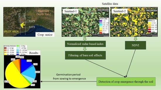
:The reliability of crop-growth modelling is related to the accuracy of the information used to describe the agricultural growing phases. A proper knowledge of sowing periods has a significant impact on the effectiveness of any analysis based on modeled crop growth. In this work, an estimation of maize actual sowing periods for year 2019 is presented, combining the optical and radar information from Sentinel-1 and Sentinel-2. The crop classification was conducted according to the information provided by local public authorities over an area of 30 km × 30 km, and 1154 maize fields were considered within the analysis. The combined use of NDVI and radar time series enabled a high-resolution assessment of sowing periods and the description of maize emergence through the soil, by detecting changes in the ground surface geometry. A radar-based index was introduced to detect the periods when plants emerge through the soil, and the sowing periods were retrieved considering the thermal energy needed by seeds to germinate and the daily temperatures before the emergence. Results show that 52% of maize hectares were sowed in late April, while about 30% were sowed during the second half of May. Sentinel-1 appears more suitable to describe the late growing phase of maize, since the radar backscattering is sensitive to the dry biomass of plants while the NDVI decreases because of the chromatic change of leaves. This study highlights the potential of synergy between remote sensing sources for agricultural management policies and improving the accuracy of crop-related modelling.
1. Introduction
The analysis of crop growing phases is essential to gather information about the factors affecting agricultural production and to adopt proper management strategies. Given the importance of agriculture in the global food system, the sensitivity of crop yields to several factors is increasingly studied through multidisciplinary approaches. Many studies are based on crop models, requiring input information at proper resolutions and spatial scales [1]. The improvement of crop modelling at different spatial scales, from local to global, is a key factor in raising awareness of drivers affecting crop yield and crop-related variables. The importance of climate variables for agricultural production is widely analyzed, particularly in terms of climate-driven impacts through the past decades [2] and of future vulnerability due to projected climate scenarios [3]. Besides climate variables, agricultural production is very sensitive also to human practices, technological improvements, and local policies [4].
Sowing periods have an important impact on the crop yield of many of the most common crops, like maize, wheat and rice [5]. Several authors analyzed the impact of late sowing on yield losses; for example, studies have shown that late sowing causes maize yield losses in the U.S. Midwest, because of increasing water stress during the vegetation and reproductive phases [6]. Similar analyses have been performed for different crops: for example, Ortiz-Monasterio et al. [7] quantified that wheat yield decreases by about 1% for every day of late sowing in Northern India, because of non-optimal climate conditions in the final growing phase. Frequently, the temporal shift of sowing and harvesting dates has been adopted as local adaptation strategy to climate change, e.g., the sorghum production in Italy [8], rice in Sri Lanka [9], soybean in Austria [10], oilseed crops in the U.S. South-West [11]; however, many limitations still constrain the adjustment of growing periods as a reliable strategy to prevent local climate-driven yield losses [12].
Earth Observation (EO) has shown a high potential to retrieve land surface parameters [13,14]. Remote sensing is increasingly used for agricultural applications because it provides data suitable for many purposes, from large-scale numerical modelling to precision farming. Techniques combining optical and radar data from satellites offer a wide range of solutions for high-resolution agricultural applications [15]. The optical data are highly sensitive to the color of the soil, to the dynamics of the vegetation cover as well as to the process of photosynthesis, while microwave instruments can detect geometric and dielectric properties of ground surfaces [16,17]. In fact, the measured signal is dependent on the radar configurations (frequency, incidence angle, and polarization) and the dielectric and geometric properties of the surface.
The study of EO as an instrument to retrieve sowing information is receiving an increasing attention. Although some sowing calendars are provided for global crop models (e.g., the MIRCA2000 gridded monthly calendars [18] or the FAO national information for irrigated crops [19]) there is still a lack of information at regional and local scale, where the spatial variability of sowing days and multi-seasonal practices is more evident. Several studies addressed the use of satellite data for the assessment of crop sowing periods in different regions of the world, combining sensors and frequency bands to describe initial phenological phases. For example, Zhang et al. [20] developed a scalable method based on MODIS data to estimate sowing periods of soybean in Mato Grosso (Brazil). EO-based methods were tested for several crops in many other regions, such as maize in South Africa [21], maize and soybean in the U.S. states of Iowa, Illinois, and Indiana [5], and wheat in India [22]. Several combinations of EO sensors have been exploited, mostly based on visible, infrared and microwave data. Recently, much attention has been given to active radar as a reliable instrument to retrieve sowing periods [23]. The analysis performed over the Bekaa Valley (Lebanon) by Nasrallah et al. [16] showed the reliability of multi-polarization active radar for the assessment of crop sowing periods.
The main research question that the present work aims to address is: can crop-specific sowing periods be retrieved/inferred from an EO-method combining active radar and optical data? The present work also aims to exploit the potential of combined optical and active radar information to describe the vegetation cycle of maize, highlighting the strengths of each sensor to detect significant properties of growing phases. To address the above goals, the high-resolution information from Sentinel-1 and Sentinel-2 have been combined with ground information on land use to analyze the growth cycle of maize over a densely cultivated temperate region in Piedmont (North-West Italy). Since maize is sowed and harvested within the same year, the analysis was carried out for the year 2019: besides the availability of data, analyzing year 2019 avoids uncertainties related to the agricultural practices during the global pandemic occurring in 2020.
In Section 2, we present the satellite data used for the study and the ground information which was used to derive the land classification. In the same section we detail the procedure adopted to identify the pilot fields, to describe the phenological cycle of maize and to derive sowing dates. In Section 3, the results of the applications are presented and discussed; first, the checking for rainfed areas in the largely irrigated region are addressed; the spatio-temporal variability of emerging and sowing periods is then discussed, comparing the results with available large-scale calendars and with the information provided by local farmers.
2. Materials and Methods
2.1. Study Site
This study aims to exploiting the potential of remote sensing information to analyze the maize growth over a densely cultivated pilot area within the province of Cuneo, in the North-West of Italy. The pilot area extends approximately from 7.47°E to 7.85°E, and from 44.34°N to 44.6°N (about 30 km × 30 km), including the municipalities shown in Figure 1.
Most of the croplands are distributed in the plain region in north-central part of the site, typically below 600 m of elevation, according to information from the Corine Land Cover classification [24] and the Digital Terrain Model provided by Regione Piemonte [25]. According to the Köppen–Geiger classification, the local climate is warm temperate, with humid summers and mean temperatures below 22 °C. The monthly hydro-climatic information provided by ISPRA [26] shows that the mean precipitation and the mean reference evapotranspiration range between 2–3.5 mm/day and 2.5–3 mm/day respectively (average values for croplands from April to October), as shown in Figure 1c,d.
The pilot area is characterized by a complex pattern of crops and an extensive network of irrigation channels. Maize is the most cultivated cereal, accounting for 65.7% of cereal areas and 17.0% of total agricultural hectares (including pastures and fallow lands), according to the Italian National Institute of Statistics (ISTAT [27]).
As shown in Figure 1f, irrigated croplands account for large parts of municipal territories, especially in the north-central part of the site, according to the Agricultural Census promoted by ISTAT in 2010 [28] (e.g., irrigated croplands are more than 80% of Morozzo and Montanera overall areas). The same Census highlights that about 90% of maize fields in the province of Cuneo are irrigated. The pilot site is equipped with a dense network of irrigation channels, belonging to 7 irrigation districts. The shape files describing the extension and the location of irrigation infrastructures and administrative areas were provided by Regione Piemonte [29]. More than 98% of irrigation channels are located within the borders of the irrigation districts. Besides the network of irrigation channels, the area is equipped with a high number of wells [30] (Figure 1g), which may provide additional water to the fields.
2.2. Satellite Data
2.2.1. Sentinel-1
The Sentinel-1 constellation acquires C-band SAR (Synthetic Aperture Radar) data, at the spatial resolution of 10 m × 10 m. The synergic acquisitions of Sentinel-1A (launched on 3 April 2014) and Sentinel-1B (launched on 25 April 2016) provide co-polarized (Vertical-Vertical, VV) and cross-polarized (Vertical-Horizontal, VH) images with a 6-days frequency and an incident angle of approximately 39° at the study site.
The Sentinel-1 data are available at different processing levels, depending on the corrections applied to the raw acquisitions. The Level-1 of Sentinel-1 data provides GDR (Ground Range Detected) images, available as gridded backscattering coefficients derived from raw signals through a processing procedure: thermal noise removal, radiometric calibration, terrain correction and speckle filtering [31].
The Sentinel-1 data used in this study were downloaded from the Google Earth Engine platform [32] as multi-band rasters in decibel units, which were pre-processed to meet the Level-1 GDR requirements [33]. The mask of maize fields shown in Figure 2a (whose characterization is discussed in Section 2.3) was used to select just the maize pixels from the SAR images. The VV and VH polarization bands were extracted from the multi-band rasters and converted from decibel (dB) to linear (lin) units:
where VVdB and VHdB are the backscatter signals provided in decibels as Level-1 SAR product; VVlin and VHlin are the backscatter signals converted into linear units, which are consistent with the units of raw acquisitions.
The SAR instrument from Sentinel-1 is an active microwave sensor, which has been shown to be sensitive to several ground variables, such as soil moisture [17,34,35] and surface geometry [36]. Both VH and VV channels can be used for crop growth monitoring, since the phenological cycle impacts the ground geometry of the fields, both in terms of roughness and biomass volume. The co-polarized signal has been shown to be more sensitive to combined surface-volume scattering, also having a high signal-to-noise ratio, while the cross-polarized channel is more suitable for detecting volumetric changes of vegetation [37].
2.2.2. Normalized SAR-Derived Index
The potential of the combined use of VH and VV for agricultural monitoring has been explored in the scientific literature. The VH/VV ratio (Figure 2b) has been shown to be a very suitable vegetation index, being able to limit the double-bounce effect caused by the vegetation ground interaction [15,16,17,37].
The effect of soil moisture and bare soil roughness can be limited by normalizing VH/VV, which is able to detect the vegetation-induced backscattering setting the minimum signal for a specific type of crop, and then filtering the soil moisture-induced noise during the bare-soil period. However, even if Sentinel-1 enables the detection of high-resolution ground geometric changes, the aim of this study is to retrieve information of generalized behaviors of crop-specific sowing, to compare the estimations with local available sowing information and general crop calendars. For this reason, a large number of fields were considered in this case, in order to perform the EO-based analysis within a representative spatial sample of the area.
For each acquisition, the average VH/VV ratio was calculated for every maize field through a GIS-based analysis. The VH/VV mean results were then converted into decibel units with:
In order to compare the signals from different maize fields, a new index called (Polarimetric Ratio Index) is proposed in this study; it is based on the normalized VH/VV ratio considering the maximum and minimum value from each field:
where the pedexes identify the maximum and minimum values of VH/VVi [–] during the growing season respectively, calculated for each i-th maize field. The index allows a direct comparison of the backscattering variability during the first part of the season, avoiding misalignments due to different ground roughness in different maize fields. The minimum equal to zero corresponds to the context of bare soil. The maximum equal to 1 corresponds to the maximum of VH/VV ratio and then to the highest vegetation volume scattering. The from pixels corresponding to each maize field (classified according to the procedure described in Section 2.3) were averaged for each acquisition day, to calculate the mean daily of every maize field.
Although the normalized combination of VV and VH has already been used for crop phenology monitoring [16], to the best of our knowledge, this is the first time that a noise-filtered index based on the normalized VH/VV was directly used to retrieve crop-specific emerging periods.
2.2.3. Sentinel-2
The Sentinel-2 constellation provides optical data at the 10 m × 10 m spatial resolution every 5 days (Figure 2c). Many indices for terrestrial monitoring can be derived from the optical information. In this work, the NDVI (Normalized Difference Vegetation Index) was used for the monitoring of vegetation changes in terms of optical and infrared signals. The NDVI index is defined as [38]:
where NIR and RED are the Near InfraRed and the RED reflectance respectively, for each i-th maize field.
The Theia-Land web service provides 10 m × 10 m cloud free NDVI data, correcting the atmospheric effect from Sentinel-2 measurements [39]. The NDVI time series were calculated by averaging the pixels corresponding to each maize field (classified according to the procedure described in Section 2.3) and interpolating the mean values for each Sentinel-2 acquisition [23,40]: a linear interpolation was performed to retrieve NDVI grids for the days between two consecutive sets of data, since NDVI changes are mainly driven by the phenological growth of plants.
2.2.4. Soil Moisture Satellite Product
The surface soil moisture (SM) was estimated by El Hajj et al. [41] from a synergy between the Sentinel-1 SAR and Sentinel-2 optical data and using neural network techniques. The S2MP product (Sentinel-1/Sentinel-2 Moisture Product) provides gridded data of soil water content [Volwater/Volsoil] over agricultural areas with 6-days frequency and a spatial resolution of 10 m × 10 m (Figure 2d). The S2MP data used in this work were downloaded from the open access service of Thisme Data Service [42]. The S2MP operational data refer to the upper soil layer (3–5 cm) and are derived both from the ascending and descending orbits of Sentinel-1, passing at the zenith at around 5:30 p.m. (ascending) and 5:30 a.m. (descending) respectively. The SM information derived from the descending orbit was not used, to avoid the effect of morning dew, in agreement with Le Page et al. [43]. The backscattering coefficient used for the S2MP estimation was obtained combining the contributions from vegetation and soil. The accuracy of the S2MP estimation was estimated to be about 6% for dry soils and up to 6.9% for very wet soils [41] and the RMSE was 1.5% higher for NDVI increasing from 0 to 0.75. The S2MP product can be applied for NDVI lower than 0.75 (for denser vegetation covers, the backscattering signal appears to be too attenuated to provide good SM estimations).
2.3. Maize Fields Characterization
The classification of agricultural fields was based on the geo-referenced information from the cadastral geodatabase of Regione Piemonte [44], which provides the shape files of all the cadastral parcels for the pilot area. First, the parcels representing agricultural areas were identified matching the cadastral shape files and the annual attribute tables from the agricultural registry of Regione Piemonte [45], which collects the annual farmer’s declarations of land use. Combining this information, each agricultural parcel was classified according to the declared cultivated crop for year 2019.
A NDVI-based filtering was performed to improve the accuracy of the maize classification: despite the shapefile of cadastral parcels identifying the maize areas, the area of many of these parcels also has non-agricultural elements (e.g., gravel roads, buildings, rows of trees). The NDVI allows consideration of only the actual agricultural pixels in each parcel, as well as checking the quality of the cadastral classification. The shape files were converted in a 10 m × 10 m raster to match the resolution of NDVI data from Theia. The pixels within the shape mask of maize parcels were analyzed in terms of NDVI response to define the borders of actual maize fields based on the NDVI signal. The values at 15-day intervals have been interpolated to obtain a daily signal from April to October.
According to El Hajj et al. [46], fully developed maize can reach NDVI values higher than 0.7, while the NDVI values for bare soil are typically lower than 0.3. The preliminary-classified fields were filtered by selecting those areas with at least 2 weeks of bare soil in the spring period (April–June) and with an increasing NDVI signal reaching values higher than 0.7 for at least 3 weeks between July and September. As a result of the filtering procedure, 1154 fields were obtained. The spatial distribution of maize fields on which the analysis described in this study is based is shown in Figure 2a, as well as the frequency distribution of the areas of the fields. As shown in Figure 2e, the NDVI series show an initial development of maize plants starting in May–June, when the optical index shows increasing values from 0.3 to 0.7. The maximum development of maize plants results for the period between late July and the first half of August.
In order to verify the effects of annual crop rotation (a widely adopted practice in this region [47]), the NDVI-based classification was performed on the same 1154 fields for the years 2018 and 2020. As shown in Figure 2e the NDVI analysis highlights that all the fields behave uniformly in 2019, indicating a correct crop classification for 2019, which is the reference year for the cadastral classification. In contrast, 34.3% of the fields harvested with maize in 2019 were shown to be cultivated with different crops in 2018 (Figure 2f); the percentage was even 36.1% in 2020 (Figure 2g).
An EO-based spatial analysis has been carried out to check for the presence of rainfed maize. Since the availability of irrigation infrastructures can have a significant impact on agricultural practices, it is important to determine if sowing calendars should be discussed separately for irrigated and rainfed maize. In this work, 159 potential rainfed maize fields were identified, selecting those outside the irrigation districts and at least 100 m from the closest irrigation channel. Still, it is possible that irrigation from water wells is operated. The results of this analysis are discussed in Section 3.1.
The NDVI responses from each maize field have been analyzed from April to October and matched with the radar backscattering signal during the same period. The signals from the fields within the irrigation districts were compared to the signals from other fields, to highlight the effect of irrigation: during the dry periods, the NDVI from rainfed maize is expected to be lower than from the irrigated maize, where the stress effect is mitigated by irrigation. Likewise, the SAR backscattering can detect differences between rainfed and irrigated fields, being sensitive to the vegetation water content.
The soil moisture data described in Section 2.2.4 were used to check for rainfed maize. For each field, the mean soil moisture was calculated for the period from May to July. The mean NDVI was calculated likewise on each field for the same growing period. According to the assumption that irrigation allows maintenance of higher levels of soil moisture during dry periods, as well as higher NDVI responses, the mean soil moisture and NDVI were compared for the fields within the irrigation districts and those far from irrigation infrastructures.
2.4. Identification of Crop Emergence and Sowing Periods
The backscattering and NDVI signals were analyzed during the maize growing season. The sensitivity of the VH/VV signal was exploited to identify the emergence periods of maize (EP), i.e., the time at which the germinating plant emerges from the ground and starts to grow. According to the NDVI series, the initial growing phase develops during May and June. Even if the NDVI signal suggests some fields are already sowed during April, the analysis of backscattering signal was performed from May, to avoid the uncertainty related to the fields still cultivated with winter crops in April.
The daily signal was compared to the NDVI for two growing stages: the initial and growing phase (May–June–July) and the middle-final phase (August–September–October). The two phases were defined according to the mean NDVI values. From May to July the NDVI increases because of the cover development, reaching the maximum between July and August. In the last three months, the NDVI gradually decreases because of the chromatic change of maize leaves, up to rapid and strong variations indicating net changes corresponding to the harvesting times.
The EP periods were identified through an approach based on the analysis of the signal. The bare soil period was identified for each field, according to the NDVI data, and the backscattering signal was calculated for this period to identify the noise from moisture and roughness variability in bare soil. For each field, the noise induced by bare soil was removed from the signal for the complete growing season, as described in Equation (5):
where is the normalized VH/VV backscattering (non-dimensional), is the filtered obtained by removing the backscattering from pure bare soil, is the backscattering during the growing season (GS), and lbp is the length of the period before plant emergence [days]. The filtered normalized backscattering, expressed as Polarimetric Ratio Index () should have values close to zero until the plants start to grow out from the ground.
The EP was assigned to each field according to the time in which the signal exceeded the 0.1 threshold. This cut-off value was fixed according to the uncertainty associated with the radar signal [48].
The maize sowing periods (SP) were inferred from the EP, considering the daily air temperature and the soil moisture conditions in the days before the emergence, as previously done by Nasrallah et al. [16]. According to the method described by Swan et al. [49], the days needed by the planted seeds to emerge from the ground were computed calculating the daily Growing Degree Units (GDU) [°C]. This indicator, also named Heat Units, describes the relation between crop development and the daily temperature. The heat accumulation, calculated considering the daily minimum and maximum temperatures, is used to measure the time required by crops to reach specific development phases.
Several authors provide estimations of the total GDU required by the maize plants to emerge through the soil: Darby and Lauer [50] calculated a GDU requirement of 69.4 °C while Abendroth et al. [51] suggested a range between 50 and 66.7 °C. For maize cultivated in the Eastern part of Po Valley (North-East Italy), a GDU requirement of 61 °C was proposed by Berti et al. [52]. In the present work, a mean GDU requirement of 62.9 °C was assumed as reference value for maize to reach the emerging phase, to be consistent with general recommended values and specific GDU estimated for Northern Italy. The daily GDU were calculated as:
where GDUi are the growing degree units for the i-th day [°C], Tmax and Tmin are the maximum and minimum air temperatures for the i-th day and Tbase is the low threshold temperature required for maize growth. According to the guidelines from the University of Wisconsin [53], Tbase was assumed equal to 10 °C and the upper and lower limits for daily Tmax and Tmin were fixed to 30 °C and 10 °C respectively. Daily temperature data provided by Arpa Piemonte [54] were used to determine the daily GDU for each field. The daily GDU were cumulated backwards from the emergence days to reach the required amount of Growing Degree Units for the crop emergence: for each field, the day on which the cumulative Growing Degree Units reached 62.9 °C was chosen as the sowing date.
According to Schneider and Gupta [55], soil moisture (SM) can affect the total GDU required by maize to reach emergence: for moisture values below the optimum in the seeding-zone, 16.7 °C should be added to the amount to be reached. Even if the impact of soil moisture occurs only in very dry periods, the optimum condition of soil water content is an important factor for the choice of sowing dates by farmers: for this reason, the impact of soil moisture on the length of emerging periods was considered in this study. The gridded moisture data described in Section 2.2.4 were used to identify moistures below optimum conditions. The upper limit of soil moisture was set for each field considering the maximum value from January 2018 to October 2021: these values were assumed as the field capacity of each field. According to the methodology described by FAO [56], each crop reach water stress conditions when soil moisture reaches values lower than specific fractions of field capacity: the FAO guidelines suggest that maize reaches stress conditions when soil moisture is lower than 45% of field capacity. The mean soil moisture during the 20 days before the plant’s emergence was calculated over each field: for the fields where the mean SM was found lower than 45% of field capacity, the GDU requirement of 62.9 °C was increased by 16.7 °C.
3. Results and Discussion
The outcomes of the analysis are described in this section and summarized as follows. First, the results of the irrigated/rainfed classification (Section 3.1) show that maize can be uniformly considered irrigated on the pilot area; in fact, the analysis performed on the fields in and outside the irrigation districts did not point to any relevant difference in the satellite time series. The results from the analysis performed throughout the growing season are discussed in Section 3.2, comparing the potential of optical and SAR data to retrieve information for different growing phases. The maize sowing periods (SP) are reported and discussed in terms of emergence periods of maize plants detected from SAR information, and the derived distribution of actual SP over the pilot area (Section 3.3).
3.1. Identification of Potential Rainfed Fields
The maize fields within and outside the irrigation districts (respectively called “in ID” and “out ID” in this section) were compared in terms of NDVI and VH/VV series. This comparison was performed to identify differences between the two groups of fields, in order to potentially calculate separate SP for rainfed and irrigated scenarios. As shown in Figure 3, the 0.25, 0.50 and 0.75 quantiles of the signals from the maize fields were computed every 6 days, to be consistent with the SAR frequency of acquisition. The quantiles series do not show any significant difference between the two groups of fields. Despite the 0.95 and 0.05 quantiles of NDVI showing a different range of values in June and September, this misalignment can be explained considering the differences between the two sets of fields: in fact, less than 14% of maize fields were considered as potentially rainfed. In addition to the numerical difference between the two groups, the potentially-rainfed fields are concentrated in areas at higher elevations and along the rivers, while the irrigated fields are more uniformly distributed over all the pilot area.
Time series of mean NDVI and VH/VV were obtained from daily mean values from Figure 3. The NDVI mean signal from fields within the irrigation districts is almost equivalent to the mean signal calculated for the other fields. The VH/VV comparison highlights a slight difference between the two groups from April to May: the mean VH/VV from fields within the irrigation districts is −0.6 dB lower, considering the two months. However, this misalignment can be considered a consequence of the noise induced by the bare soil geometry, since the difference gradually reduces when the VH/VV become more sensitive to the growth of the plants.
A further comparison was performed between the two groups of fields, considering the complete series of NDVI and VH/VV among the growing season. Even if the temporal mean signals from the two groups of fields are well aligned, the effect of irrigation could lead to more evident divergences considering the long-term effect during the full growing season. The sum of the mean daily NDVI from April to October was compared for the fields within and outside the ID: a misalignment of −0.01% was found between the sums of the two mean NDVI signals. The same analysis shows a misalignment of −1.7% from April to October between the sum of mean VH/VV within and outside the ID, and a misalignment of −0.4% considering the period from June to October (when the irrigation season is concentrated, and the effect of bare soil is limited). In both cases, the analysis did not point out any appreciable differences between the two groups of fields.
The monthly correlations between NDVI and VH/VV were calculated for the two groups of fields, to identify potential impacts of irrigation limited to the areas of the irrigation districts. The analysis was performed for the first part of the maize growing cycle, when the VH/VV is still sensitive to the soil moisture anomalies induced by irrigation since growing plants still do not cover entirely the ground. Table 1 shows the monthly Pearson correlation coefficients (obtained dividing the covariance by the product of the two variables’ standard deviations) considering all the signals retrieved every 6 days from all the fields of each group. The mean monthly NDVI was also compared with the mean soil moisture retrieved over the two groups of fields. The comparison does not show any appreciable difference between the maize fields cultivated within or outside the irrigation districts.
3.2. Growing Phases
The analysis performed throughout the growing season showed some relevant results in terms of optical and radar performance in the monitoring of maize growth. The comparison between NDVI and VH/VV shows a good alignment in the remote sensing responses during the initial growing phases, as shown in Figure 3. From May to July the NDVI increases from about 0.2 to the maximum values (0.75–0.9) and the VH/VV backscattering also increases from −10 dB to −5 dB on average. Although the NDVI decreases significantly during the final phase (September–October), there is no evidence of an analogue decrease in terms of backscattering. Since the NDVI is derived from visible and near infrared frequencies, the strong decrease is driven by changes in the chromatic response of maize leaves. However, the VH/VV does not appear to be affected by an analogous decrease during the same period; in fact, the backscattering signal is sensitive to changes in the ground coverage structure and water content.
Since VH/VV shows a low decrease during September and October, we can assume that this response is driven by the decrease of plant water content and the progressive drying of maize leaves. Yet, the signal decreases “slowly” because of the presence of dry biomass on the ground inducing volume scattering. This misalignment between NDVI and radar backscattering in the final part of the growing season is particularly meaningful for those algorithms retrieving soil moisture values based on NDVI information: since the plants’ height affects the reliability of soil moisture results, these models usually suggest specific ranges of NDVI for which the soil moisture can be used. However, according to the results from Figure 3, any analysis whose reliability is affected by the plant coverage would be more robust taking into account the response of the dry biomass, to which radar is more sensitive than optical measurements.
The maize growth was also analyzed in terms of the normalized backscattering signal (). The scatterplots in Figure 4 show the relation between (i.e., the normalized VH/VV backscattering) and NDVI along two main growing phases. In the first growing phase (May–June–July), most of the maize fields appear to be already sowed and the development of plants corresponds to the NDVI changes and the response. NDVI increases are due to the visible and near infrared signals of the land cover.
In the first part of the phase, when the NDVI is still lower than 0.25 (bare soil), the variability of is mainly due to changes in the soil moisture and roughness due to the incipient growth of maize plants. The first consequence of maize emerging, before any response in terms of NDVI, is the change of ground roughness, to which the normalized backscattering is very sensitive. NDVI is more sensitive to chromatic responses of vegetation coverages instead of roughness variability, and the seedlings of freshly born maize do not provide any significant change in the optical response during the early days of growth. In fact, as shown in Figure 4a, the daily comparison between NDVI and highlights a range of values where starts to grow quickly but NDVI appears to be less sensitive (i.e., May, during the first part of the growing season). The results in Figure 4 show the distribution of daily NDVI and month-by-month over the pilot area: the distribution of the increments seem to indicate that the emerging phase starts in early May and continues up to late June; in fact, even if most of the blue crosses reach high values of during May (Figure 4a), there are still some fields where the plants break through the soil during June (green circles, Figure 4a).
During the later growing phase, from August to October (Figure 4b), the NDVI starts to decrease because of changes in the chromatic response of maize leaves. During August plants have reached the maximum height of development and there is no significant NDVI variability (blue crosses, Figure 4b). Despite NDVI markedly changing in this period (values from 0.9 to 0.2), the daily variability of appears to be lower.
The NDVI decrease from August to October is directly correlated to the vegetation’s water content: maize plants become gradually drier during the final phase of the growing season, with a different response in terms of red and infrared reflectance. However, the SAR backscattering depends both on the vegetation water content and the geometric structure of the ground coverage.
During the final growing phase, the misalignment between NDVI and decreases is due to the sensitivity of the radar backscattering to dry biomass covering the ground, which limits the variation compared to NDVI. Sudden decreases in the VH/VV signal to low values may be due to the maize harvesting over some of the fields, during September and October (orange triangles and green circles in Figure 4b).
3.3. Emerging of Plants and Sowing Periods
In order to identify the periods in which maize starts to grow, the SAR data were analyzed for the period from May to June. The mean and variance of VH/VV over time in each field are shown in Figure 5: each point in the scatterplot represents the VH/VV statistics from May to June, colored according to the mean NDVI calculated for the same period.
Fields where maize is sown in the early May (or even in April) show a lower variance of VH/VV, because the growth of plants tends to produce a uniform field coverage. For the same reason, the early sowed fields show a higher mean backscattering and a higher mean NDVI, because the growing phase is at a later stage and plants are more developed. The presence of different mean NDVI classes over the May–June period may indicate that maize was sowed in distinct phases. About 25% of maize fields appear to have a mean NDVI lower than 0.3 in the first two months: for these fields, the NDVI was typically higher than 0.3 during April, meaning that winter crops planted on the same plots before maize were probably still cultivated until this time.
A high VH/VV variance is typical of scenarios where maize plants break through the soil. The low height of plants corresponds to low NDVI, but also to high variability of ground coverage due to the incipient growing phase, to which VH/VV is sensitive.
The normalized backscattering signal () was filtered to limit the sensitivity of radar data to the variability of bare soil water content, according to the procedure described in Section 2.2.2. The variability of the filtered signal () is mainly a consequence of geometric changes on the ground surface, which is typically related to the emerging of maize plants during the first part of the season. The emergence time was identified according to the temporal series of , checking the time in which the filtered backscattering exceeds the threshold of 0.1. The bar plot in Figure 6 shows the distribution of the emergence periods (EP). Most of the maize reaches the soil surface in the second half of May, especially between 12th and 18th of May. The distribution of EP highlights the presence of a second main emergence period, between the last days of May and the beginning of June.
It is interesting to observe that maize appears to be sown earlier at low elevations (h < 400 m above the sea level) than at higher elevations. In fact, plants break through the soil between the end of May and mid-June on the fields higher than 500 m, which are characterized by lower temperatures than areas at lower elevations.
The presence of two different SP is consistent with the typical agricultural practices of the area, where winter crops are harvested in late spring. These crops may be present on those fields which are sown later at the lower altitudes, while the time shift at high elevations may depend on the later warming of weather conditions.
Despite some areas appears to be sowed in the first week of April, this practice is not widespread over the region. The early sowing is mostly related to the grain maize, which requires longer periods to grow and reach the optimum water content in the final product at the end of the season, and to local insurance policies that refund maize farmers in case of late frosts in April.
According to the methodology described in Section 2.4, the actual sowing dates were estimated by inverting the method for the calculation of the emerging period from the sowing date, according to daily temperatures and soil water content. Considering that emergence periods can be calculated on a 6-days interval, because of the revisiting time of Sentinel-1 data, the estimation of actual sowing dates is affected by the same uncertainty; in Figure 7, results are presented with such temporal resolution.
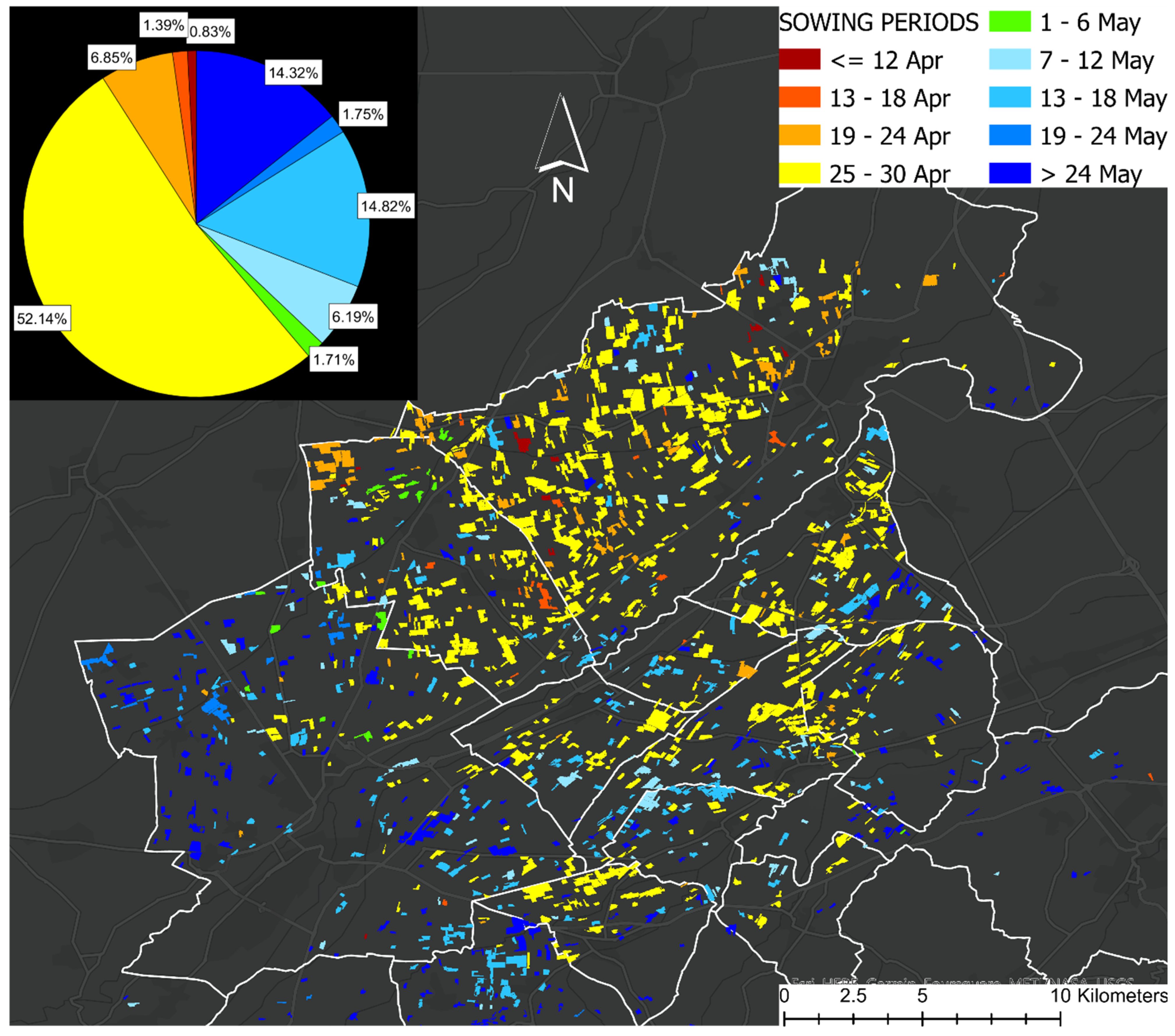
More than 52% of maize areas are sowed in the last six days of April, especially in the northern municipalities where this percentage is higher than 70% (e.g., 78% in Fossano, 73% in Sant’Albano Stura). About 9.1% of maize fields are sowed in the remaining days of April. About 30% of maize areas were sowed in the second half of May and at least 9% during the first half of the month.
The spatial distribution of maize SP highlights that, on average, the fields at lower elevations are sowed earlier (see the DTM map in Figure 1b). A statistical analysis was performed to calculate the correlation between the SP and the topographic elevation: the 6-days intervals, consistently with the Sentinel-1 revisiting time, were numbered for year 2019 (e.g., April 13th–18th interval is the 18th group of 6 days from the beginning of the year); for each field, the numbered 6-days period was compared to the elevation (in terms of meters above the mean sea level). The Pearson correlation coefficient (R), which quantifies the correlation strength between two sets of variables (ranging from 0 to ±1), shows a moderate positive correlation of 0.41 between sowing periods and topographic elevation (according to the classes of correlation proposed by Evans in 1996 [57]). In fact, despite an evident gradient of sowing periods moving from lower to higher altitudes, a significant part of fields at low altitudes appears to be sown during May. This can be explained by some declarations from local farmers, stating that fields at low elevations have a higher probability to be cultivated with winter crops until April (Appendix A): this could be the main reason for the coexistence of fields sowed on early April and late May at elevations <450 m above the sea, where medium temperatures are higher.
The results of sowing periods are consistent with the information collected from local farmers (interviewed by the authors in November 2021) who declared that maize is usually sowed twice per season, in April and May, according to the agronomic variety of plants and the use for which the product is intended. The maize sowed in April is usually a high-quality product for the food market, while the plants sowed in May are those to produce mash corn for farm animals. The results obtained in this study fit well with the available sowing information described by previous studies in Northern Italy. Berti et al. [52] collected sowing periods over 6 sites in North-East Italy, from 2005 to 2007: local farmers declared that maize was mostly sown during late April in 2005 (sowing occurred between 27 April and 1 May in 3 of the 6 sites). Despite a slight temporal variability, this study states that most of the maize was sown in April also in 2006 and 2007. Even if the data were collected in the eastern part of Po Valley, the agricultural practices can be assumed as sufficiently uniform in the densely cultivated region of Northern Italy. Moreover, also the regional calendar provided by Azar et al. [58] considers April as the sowing month for maize in Northern Italy, and the second week of May as the reference emergence period of plants.
Although global sowing calendars can only be used as general reference information and not as actual data for validation, the results obtained in this study fit well with the large-scale SP for irrigated maize provided by the crop calendars from FAO [19] and MIRCA2000 [18]. The FAO calendar indicates April as main sowing month for irrigated maize, with high probability that a small part of irrigated croplands may be sowed later. The U.S. Department of Agriculture provides monthly information for crop-specific sowing dates worldwide [59]: this calendar states that April is the main sowing period for maize in Italy.
The main limitation of this work is the lack of information about actual sowing dates at the field scale, to be used for the validation of results validation: right now, results can only be compared with local declarations from farmers and large-scale calendars. As previously mentioned, local farmers were asked to answer a survey to get an overview of the maize cultivation practices in the pilot area, in order to partially fill this gap. The results of the survey are available in Appendix A, within the Supplementary Material of this study. Although this source is too scattered to be used for an actual validation, the information collected from farmers was a valuable source in giving confirmation of the results.
4. Conclusions
The sowing period has been proven to have an important impact on the yield of many of the most common crops, especially cereals. Moreover, the shifting of agricultural sowing periods is increasingly used as an adaptation strategy to climate change.
In this work, the reliability of Earth Observation to retrieve maize sowing periods was tested, analyzing a pattern of 1154 fields within a 30 km × 30 km area in Piedmont (North-West Italy) for year 2019. Radar and optical acquisitions from Sentinel-1 and Sentinel-2, respectively, were used to classify maize fields and to detect crop emergence through the soil, building up the spatial distribution of sowing periods at the field scale. For this reason, a SAR-based normalized index (named Polarimetric Ratio Index, IPR) was proposed in this study, in order to detect the geometric changes on ground surface induced by maize emergence.
Results show that in 2019 maize was sown within April and May: about 52% of maize hectares were sown between April 25th and 30th, and 31% from May 13th to the end of May. The late sowings are more frequent at higher elevations: a moderate correlation was found between emergence delay and elevation above the sea level (Pearson correlation coefficient, R = 0.41). The maize sowed in May at lower elevations is likely cultivated on those fields where winter crops are harvested in late spring, according to a widespread agricultural practice in this area.
The comparison with actual data of local sowing practices highlights a good alignment with sowing periods occurring in the Po Valley in previous years (period 2005–2007). Results fit well with the sowing periods declared by local farmers within a survey conducted by the authors, in which the second half of April and May were indicated as the two main sowing periods. Results from this study are also well aligned to the most widely used comprehensive crop calendars, such as the global dataset of sowing periods proposed by FAO.
Although the combined use of SAR polarizations has been previously used for agricultural applications, the novelty of this approach relies on the use of a normalized SAR-based index, which allows filtering out the effect of bare soil and clearer detection of the signals induced by crop growth. Further analyses combining more satellite constellations and ground information for validation, could exploit the EO-based methodology proposed in this study to assess more precise sowing periods for various crops.
For the future, even temperate areas are expected to suffer lack of water and yield losses, because of changes in the precipitation regimes and withdrawable water for irrigation. Remote sensing is a very useful tool to support effective adaptation strategies to climate change, especially in those regions where new agricultural mindsets are increasingly required.
Supplementary Materials
The following supporting information can be downloaded at: https://www.mdpi.com/article/10.3390/rs14153712/s1.
Author Contributions
Conceptualization, M.Z. and M.R.; methodology, M.Z. and M.R.; software and resources, M.R., M.Z. and E.A.; data curation, N.B. and M.R.; writing—original draft preparation, M.R.; writing—review and editing, M.Z., S.T. and P.C.; supervision, M.Z., S.T. and P.C. All authors have read and agreed to the published version of the manuscript.
Funding
This research was funded through the 4000126684/19/I-NB CCN3 ESA project. The research funds covered the visiting period spent by the first author at CESBIO (Centre d’Etudes Spatiales de la Biosphère, Toulouse, FR).
Data Availability Statement
The data that support the findings of this study are openly available. The source of each dataset is detailed in Section 2, including links and references. No lab/field measurements were performed to achieve the aims of this study.
Acknowledgments
The authors acknowledge the CESBIO research center for the sharing knowledge and for the funding support throughout this valuable collaboration. The authors are also grateful to Michel Le Page (CESBIO), for the time he has dedicated to the authors and for sharing his GIS skills. A special acknowledgement goes to Roberto Gramaglia, coordinator of the Brobbio-Pesio irrigation district (Piedmont, Italy), for the time that he dedicated to the authors so that they could collect information from local farmers (Appendix A).
Conflicts of Interest
The authors declare no conflict of interest.
Appendix A
In November 2021, five farmers from the Brobbio-Pesio irrigation district (South Piedmont, Italy) were asked to answer a survey about maize cultivation practices and sowing periods.
Answers provided by the farmers to each question (e.g., F1: answer from Farmer 1) were as follows.
- Question 1. In which period of the year is maize usually sown?
- 1.
- F1. Usually, maize is sown twice per year. The first sowing is between the 10th and 30th of April; the second sowing occurs between the end of May and the first half of June. The choice of the sowing date depends mainly on soil moisture and weather conditions: soil temperature must be equal or above 13 °C, and there must be low risk of late frost.
- 2.
- F2. Maize is usually sown during the second half of April, or between 15 May and the first week of June. The period depends on the final product to be obtained (chopped maize or dry grain). The choice of sowing day is mainly driven by meteorological factors and soil temperature.
- 3.
- F3. According to the soil moisture and weather conditions, maize is sown from the beginning of April. The provider of seeds insures farmers against late frost: if the plant growth is blocked by late frosts in April, a new sowing can be done for free.
- 4.
- F4. If the soil moisture and weather conditions are optimal, the sowing period starts during the second half of April.
- 5.
- F5. Two growing seasons are usually planned. The first starts in April (usually during the last two weeks) and the second starts in late May.
- Question 2. In which period of the year is maize usually harvested?
- 1.
- F1. Usually between September and October (e.g., October in 2021). The harvesting period depends on the intended use of maize, for which grains must reach optimum levels of moisture. A moisture of 30%–35% is required for chopped maize; a moisture of 25% is required for dry grain at the harvesting date (after that, grains are left to dry up to 12%).
- 2.
- F2. Chopped maize is usually harvested around 15 September. Dry grain maize is usually harvested around the middle of October.
- 3.
- F3. The most crucial factor is the optimum moisture of maize grains. Usually, the maize growing season is 120–130 days long.
- 4.
- F4. From the second half of September to late October, according to the required moisture of maize seeds and on weather conditions.
- 5.
- F5. Chopped maize is usually harvested at the beginning of September. The harvesting period for dry grain maize is usually October.
- Question 3. How are maize fields used during rest periods? (e.g., fallow lands, other crops)
- 1.
- F1. Fields are usually cultivated with fodder grasses or winter wheat from autumn to spring. Typically, the rotation scheme for these months is: 1 year of winter wheat and then 3 consecutive years of fodder grasses. Maize is not cultivated in summer after winter wheat, because wheat is harvested in July.
- 2.
- F2. The crop rotation involves fodder grasses and barley (all cultivated in summer). The scheme is 5–6 years of fodder grasses, 1–2 years of maize, 1–2 years of barley.
- 3.
- F3. Maize fields are usually lying fallow during winter.
- 4.
- F4. Croplands are located at high elevations, close to the Alps. Nothing is cultivated during winter.
- 5.
- F5. Crop rotation is a summer practice. During winter, croplands are cultivated with fodder grasses.
- Question 4. Approximately, how long do the plants take to reach the maximum stage of growth from seed?
- 1.
- F1. The maximum growing stage is reached by maize in the second half of July for those years when seeds are sown around 15 April.
- 2.
- F2. Between June 20th and the first week of July, according on the date of sowing.
- 3.
- F3. The maximum stage of growth is usually reached in the first two weeks of July.
- 4.
- F4. The maximum stage of growth is usually reached in the first two weeks of July.
- 5.
- F5. According to the maize variety, the maximum growing phase is reached in mid-July.
References
- Pasquel, D.; Roux, S.; Richetti, J.; Cammarano, D.; Tisseyre, B.; Taylor, J.A. A review of methods to evaluate crop model performance at multiple and changing spatial scales. Precis. Agric. 2022, 23, 1489–1513. [Google Scholar] [CrossRef]
- Rolle, M.; Tamea, S.; Claps, P. Climate-driven trends in agricultural water requirement: An ERA5-based assessment at daily scale over 50 years. Environ. Res. Lett. 2022, 17, 044017. [Google Scholar] [CrossRef]
- Rosenzweig, C.; Elliot, J.; Deryng, D.; Ruane, A.C. Assessing agricultural risks of climate change in the 21st century in a global gridded crop model intercomparison. Proc. Natl. Acad. Sci. USA 2014, 11, 3268–3273. [Google Scholar] [CrossRef] [Green Version]
- Liu, P. The future of Food and Agriculture: Trends and Challenges; FAO: Rome, Italy, 2017. [Google Scholar]
- Urban, D.; Guan, K.; Jain, M. Estimating sowing dates from satellite data over the US Midwest: A comparison of multiple sensors and metrics. Remote Sens. Environ. 2018, 211, 400–412. [Google Scholar] [CrossRef]
- Irwin, S.; Good, D.; Newton, J. Early Planting and 2015 Corn Yield Prospects: How Much of an Increase? Farmdoc Dly. 2015, 5, 169–184. [Google Scholar]
- Ortiz-Monasterio, J.I.; Dhillon, J.; Fisher, S. RA Date of sowing effects on grain yield and yield components of irrigated spring wheat cultivars and relationships with radiation and temperature in Ludhiana, India. Field Crop. Res. 1994, 37, 169–184. [Google Scholar] [CrossRef]
- Howden, S.; Soussana, J.; Tubiello, F. Adapting agriculture to climate change. Proc. Natl. Acad. Sci. USA 2007, 104, 19691–19696. [Google Scholar] [CrossRef] [Green Version]
- Dharmarathna, W.; Herath, S.; Weerakoon, S. Changing the planting date as a climate change adaptation strategy for rice production in Kurunegala district, Sri Lanka. Sustain. Sci. 2014, 9, 103–111. [Google Scholar] [CrossRef]
- Alexandrov, V.; Eitzinger, J.; Cajic, J.; Oberforster, M. Potential impact of climate change on selected agricultural crops in north-eastern Austria. Glob. Chang. Biol. 2002, 8, 373–389. [Google Scholar] [CrossRef]
- Baldwin, B.; Cossar, R. Castor yield in response to planting date at four locations in the south-central United States. Ind. Crops Prod. 2009, 29, 316–319. [Google Scholar] [CrossRef]
- Shah, H.; Siderius, C.; Hellegers, P. Limitations to adjusting growing periods in different agroecological zones of Pakistan. Agric. Syst. 2021, 192, 103184. [Google Scholar] [CrossRef]
- Colliander, A.; Reichle, R.; Crow, W.; Cosh, M.H.; Chen, F.; Chan, S.; Das, N.N.; Bindlish, R.; Chaubell, J.; Kim, S.; et al. Validation of soil moisture data products from the NASA SMAP mission. IEEE J. Sel. Top. Appl. Earth Obs. Remote Sens. 2021, 15, 364–392. [Google Scholar] [CrossRef]
- Weiss, M.; Jacob, F.; Duveiller, G. Remote sensing for agricultural applications: A meta-review. Remote Sens. Environ. 2020, 236, 111402. [Google Scholar] [CrossRef]
- Quaadi, N.; Jarlan, L.; Ezzahar, L.; Zribi, M.; Zribi, M.; Khabba, S.; Bouras, E.; Bousbih, S.; Frison, P.L. Monitoring of wheat crops using the backscattering coefficient and the interferometric coherence derived from Sentinel-1 in semi-arid areas. Remote Sens. Environ. 2020, 251, 112050. [Google Scholar]
- Nasrallah, A.; Baghdadi, N.; El Hajj, M.; Darwish, T. Sentinel-1 Data for Winter Wheat Phenology Monitoring and Mapping. Remote Sens. 2019, 11, 2228. [Google Scholar] [CrossRef] [Green Version]
- Pascale, C.; Dubois, P.; Van Zyl, J.; Engman, T. Measuring soil moisture with imaging radars. IEEE Trans. Geosci. Remote Sens. 1995, 33, 915–926. [Google Scholar]
- Portmann, F.; Siebert, S.; Döll, P. MIRCA2000—Global monthly irrigated and rainfed crop areas around the year 2000: A new high-resolution data set for agricultural and hydrological modeling. Glob. Biogeochem. Cycles 2010, 24. [Google Scholar] [CrossRef]
- Frenken, K.; Gillet, V. Irrigation Water Requirement and Water Withdrawal by Country; FAO: Rome, Italy, 2012. [Google Scholar]
- Zhang, M.; Abrahao, G.; Cohn, A.; Campolo, J.; Thompson, S. A MODIS-based scalable remote sensing method to estimate sowing and harvest dates of soybean crops in Mato Grosso, Brazil. Heliyon 2021, 7, e07436. [Google Scholar] [CrossRef]
- Rezaei, E.; Ghazaryan, G.; González, J.; Cornish, N.; Dubovyk, O.; Siebert, S. The use of remote sensing to derive maize sowing dates for large-scale crop yield simulations. Int. J. Biometeorol. 2021, 65, 565–576. [Google Scholar] [CrossRef]
- Lobell, D.; Sibley, A.; Ortiz-Monasterio, I.J. Extreme heat effects on wheat senescence in India. Nat. Clim. Chang. 2012, 2, 186–189. [Google Scholar] [CrossRef]
- Bousbih, S.; Zribi, M.; Lili-Chabaane, Z.; Baghdadi, N.; El Hajj, M.; Gao, Q.; Mougenot, B. Potential of Sentinel-1 Radar Data for the Assessment of Soil and Cereal Cover Parameters. Sensors 2017, 17, 2617. [Google Scholar] [CrossRef] [Green Version]
- Copernicus European Programme, Land Service. CORINE Land Cover: CLC_2018 v.2020_20u1. Available online: https://land.copernicus.eu/pan-european/corine-land-cover (accessed on 11 October 2021).
- Regione Piemonte. GEO-Piemonte: Modello Digitale del Terreno da CTRN 1:10,000 (Passo 10 m)—STORICO. Available online: https://www.geoportale.piemonte.it/geonetwork/srv/ita/catalog.search#/metadata/r_piemon:3ffe6b7b-9abe-4459-8305-e444e8eb197c (accessed on 20 November 2021).
- Braca, G.; Bussettini, M.; Lastoria, B.; Mariani, S.; Piva, F. Il bilancio idrologico GIS based a scala nazionale su griglia regolare—BIGBANG: Metodologia e stime. Rapporto sulla disponibilità naturale della risorsa idrica Rapp. ISPRA 2021, 339, 1–181. [Google Scholar]
- ISTAT. Agricultura. Available online: https://www.istat.it/it/agricoltura?dati (accessed on 25 November 2021).
- ISTAT. 6° Censimento Agricoltura 2010: Data Warehouse. Available online: http://dati-censimentoagricoltura.istat.it/Index.aspx (accessed on 14 October 2021).
- Regione Piemonte. Bonifica e Irrigazione (SIBI). Available online: https://www.regione.piemonte.it/web/temi/agricoltura/agroambiente-meteo-suoli/bonifica-irrigazione-sibi (accessed on 13 November 2021).
- Regione Piemonte. Sistema Informativo Risorse Idriche (SIRI). Available online: http://www.regione.piemonte.it/siriw/cartografia/mappa.do;jsessionid=E4D50E350BDDEF87B8B00E2144523402.part212node11 (accessed on 13 November 2021).
- ESA Sentinels. Sentinel-1, Level-1 GRD Products. Available online: https://sentinels.copernicus.eu/web/sentinel/technical-guides/sentinel-1-sar/products-algorithms/level-1-algorithms/ground-range-detected (accessed on 16 December 2021).
- Gorelick, N.; Hancher, M.; Dixon, M.; Ilyushchenko, S.; Thau, D.; Moore, R. Google Earth Engine: Planetary-scale geospatial analysis for everyone. Remote Sens. Environ. 2017, 202, 18–27. [Google Scholar] [CrossRef]
- Google Earth Engine. Sentinel-1 Algorithms, Google 2022. Available online: https://developers.google.com/earth-engine/guides/sentinel1 (accessed on 20 May 2022).
- Engman, E. Applications of microwave remote sensing of soil moisture for water resources and agriculture. Remote Sens. Environ. 1991, 35, 213–226. [Google Scholar] [CrossRef]
- Zribi, M.; Baghdadi, N.; Holah, N.; Fafin, O.; Guérin, C. Evaluation of a rough soil surface description with ASAR-ENVISAT radar data. Remote Sens. Environ. 2005, 95, 67–76. [Google Scholar] [CrossRef]
- Evans, D.; Farr, T.; Zyl, J. Estimates of surface roughness derived from synthetic aperture radar (SAR) data. IEEE Trans. Geosci. Remote Sens. 1992, 30, 382–389. [Google Scholar] [CrossRef]
- Veloso, A.; Mermoz, S.; Bouvet, A.; Le Toan, T.; Planells, M.; Dejoux, J.F.; Ceschia, E. Understanding the temporal behavior of crops using Sentinel-1 and Sentinel-2-like data for agricultural applications. Remote Sens. Environ. 2017, 199, 415–426. [Google Scholar] [CrossRef]
- Rouse, J.; Haas, R.; Schell, J.; Deering, D. Monitoring the Vernal Advancement and Retrogradation (Green Wave Effect) of Natural Vegetation; No. NASA-CR-132982; Texas A and M University, College Station. Remote Sensing Center: College Station, TX, USA, 1973. [Google Scholar]
- Theia. Value-Adding Products and Algorithms for Land Surfaces. Available online: https://www.theia-land.fr/en/homepage-en/ (accessed on 15 November 2021).
- Ayari, E.; Kassouk, Z.; Lili-Chabaane, Z.; Baghdadi, N.; Bousbih, S.; Zribi, M. Cereal crops soil parameters retrieval using L-band ALOS-2 and C-band Sentinel-1 sensors. Remote Sens. 2021, 13, 1393. [Google Scholar] [CrossRef]
- El Hajj, M.; Baghdadi, N.; Zribi, M.; Bazzi, H. Synergic Use of Sentinel-1 and Sentinel-2 Images for Operational Soil Moisture Mapping at High Spatial Resolution over Agricultural Areas. Remote Sens. 2017, 9, 1292. [Google Scholar] [CrossRef] [Green Version]
- THISME. THeia and Irstea Soil MoisturE Catalog. Available online: https://thisme.cines.teledetection.fr/home (accessed on 31 October 2021).
- Le Page, M.; Jarlan, L.; El Hajj, M.; Zribi, M.; Baghdadi, N.; Boone, A. Potential for the Detection of Irrigation Events on Maize Plots Using Sentinel-1 Soil Moisture Products. Remote Sens. 2020, 12, 1621. [Google Scholar] [CrossRef]
- Regione Piemonte. GEO-Piemonte: Mosaicatura Catastale di Riferimento Regionale. Available online: https://www.geoportale.piemonte.it/cms/progetti/progetto-mosaicatura-catastale (accessed on 12 October 2021).
- Regione Piemonte. Anagrafe Agricola Unica—Data Warehouse e Open Data. Available online: http://www.sistemapiemonte.it/fedwanau/elenco.jsp (accessed on 14 October 2021).
- El Hajj, M.; Baghdadi, N.; Bazzi, H.; Zribi, M. Penetration analysis of SAR signals in the C and L bands for wheat, maize, and grasslands. Remote Sens. 2019, 11, 31. [Google Scholar] [CrossRef] [Green Version]
- Regione Piemonte. Norme Tecniche di Produzione Integrata: Difesa, Diserbo e Pratiche Agronomiche 2018. Available online: https://www.regione.piemonte.it/web/sites/default/files/media/documenti/2018-11/norme_tecniche_piemonte_2018.pdf (accessed on 5 February 2022).
- Muth, L.; Diamond, D.; Lelis, J. Uncertainty Analysis of Radar Cross Section Calibration at Etcheron Valley Range; Technical Note (NIST TN) 1534; National Institute of Standards and Technology: Gaithersburg, MD, USA, 2004.
- Swan, J.B.; Schneider, E.C.; Moncrief, J.F.; Paulson, W.H.; Peterson, A.E. Estimating corn growth, yield, and grain moisture from air growing degree days and residue cover. Agron. J. 1987, 79, 53–60. [Google Scholar] [CrossRef]
- Darby, H.; Lauer, J. Plant Physiology: Critical Stages in the Life of a Corn Plant. Technol. Rep. 2004. Available online: http://corn.agronomy.wisc.edu/Management/pdfs/CriticalStages.pdf (accessed on 17 February 2022).
- Abendroth, L.J.; Elmore, R.W.; Boyer, M.J.; Marlay, S.K. Corn Growth and Development, 1st ed.; Iowa State University, University Extension: Ames, IA, USA, 2011. [Google Scholar]
- Berti, A.; Maucieri, C.; Bonamano, A.; Borin, M. Short-term climate change effects on maize phenological phases in northeast Italy. Italy J. Agron. 2019, 14, 222–229. [Google Scholar] [CrossRef]
- Corn Agronomy. Corn Development. Available online: http://corn.agronomy.wisc.edu/Management/L011.aspx (accessed on 25 February 2022).
- Arpa Piemonte. Annali Meteorologici ed Idrologici. Available online: https://www.arpa.piemonte.it/rischinaturali/accesso-ai-dati/annali_meteoidrologici/annali-meteo-idro/annali-meteorologici-ed-idrologici.html (accessed on 21 February 2022).
- Schneider, E.C.; Gupta, S.C. Corn emergence as influenced by soil temperature, matric potential, and aggregate size distribution. Soil Sci. Soc. Am. J. 1985, 49, 415–422. [Google Scholar] [CrossRef]
- Allen, R.G.; Pereira, L.S.; Raes, D.; Smith, M. Crop Evapotranspiration-Guidelines for computing crop water requirements-FAO Irrigation and drainage paper 56. FAO Rome 1998, 300, D05109. [Google Scholar]
- Evans, J. Straightforward Statistics for the Behavioral Sciences, 1st ed.; Thomson Brooks/Cole Publishing Co.: Belmont, CA, USA, 1996. [Google Scholar]
- Azar, R.; Villa, P.; Stroppiana, D.; Crema, A.; Boschetti, M.; Brivio, P.A. Assessing in-season crop classification performance using satellite data: A test case in Northern Italy. Eur. J. Remote Sens. 2016, 49, 361–380. [Google Scholar] [CrossRef] [Green Version]
- U.S. Department of Agriculture, Foreign Agricultural Service. IPAD Crop Calendars. Available online: https://ipad.fas.usda.gov/ogamaps/cropcalendar.aspx (accessed on 2 March 2022).
Figure 1.
Characterization of the pilot area: location, elevation above mean sea level, climate, croplands, irrigation districts. (a) Location and limits of the pilot area (7.47°E to 7.85°E, 44.34°N to 44.6°N): 15 municipalities in the province of Cuneo (North–West Italy). (b) Spatial elevation above the sea level [m], 10 m × 10 m resolution. (c) Mean daily precipitation [mm/day] from April to October (average 1970–2019). (d) Mean daily reference evapotranspiration [mm/day] from April to October (average 1970–2019). (e) Land classification of the pilot area, according to the Corine Land Cover (2018) information. (f) Fractions of irrigated croplands [%] with respect to the overall municipal areas: Rocca de’ Baldi (1), Fossano (2), Boves (3), Morozzo (4), Peveragno (5), Margarita (6), Cuneo (7), Montanera (8), Pianfei (9), Mondovì (10), Castelletto Stura (11), Beinette (12), Centallo (13), Sant’Albano Stura (14), Chiusa di Pesio (15). (g) Irrigation districts and infrastructures, including rain gauges.
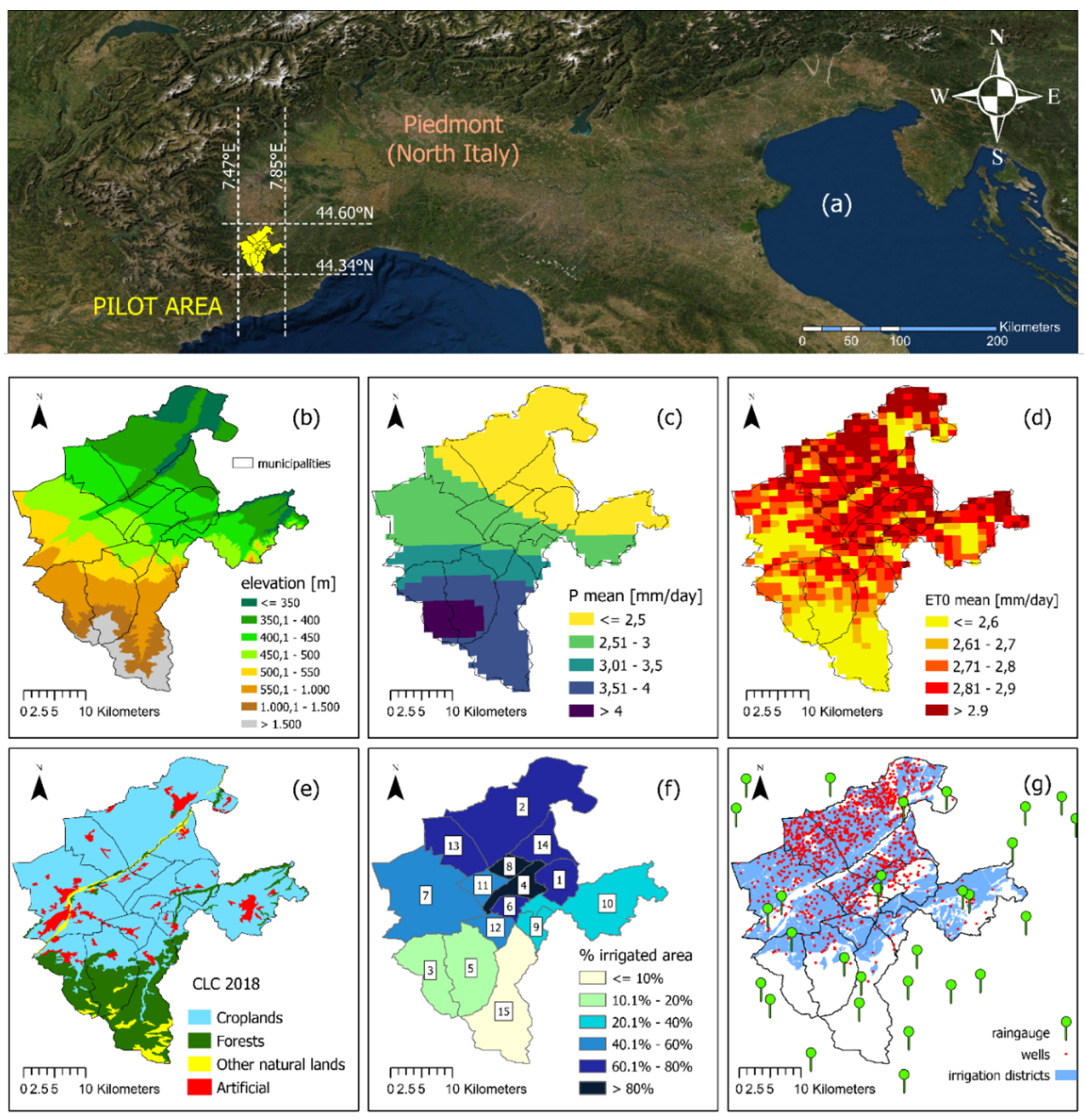
Figure 2.
(a) Spatial distribution of maize fields over the studied region and frequency distribution of field areas. (b) Example of VH/VV 10 × 10 m data over the maize fields. (c) Example of NDVI 10 m × 10 m data over the maize fields. (d) Example of soil moisture 10 m × 10 m data over the maize fields. (e) NDVI series for 1154 fields classified as “maize” in 2019. Comparison with NDVI from same fields in 2018 (f) and 2020 (g).
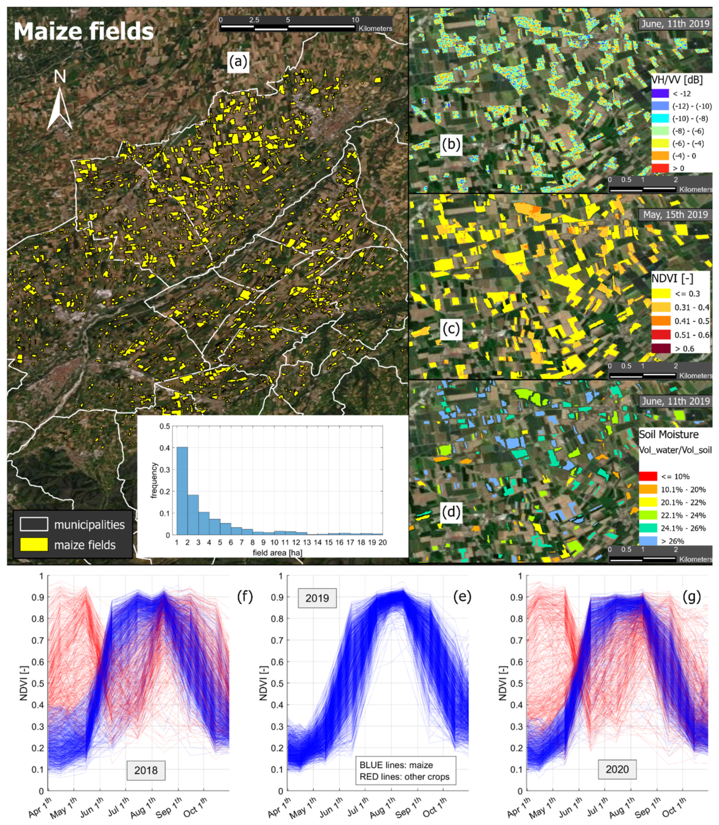
Figure 3.
Time series of NDVI values (interpolation of 15-days revisit time) and VH/VV backscattering signal (6-days revised time). Each boxplot represents the distribution of values of NDVI and VH/VV from all the maize fields. The horizontal blue lines in the boxplots represent the 25%, 50%, and 75% quantiles, respectively (from the ground up). The black lines above and under each boxplot include the values within 95% and 5% quantiles, respectively. The blue dots represent the outlier values. In the two lowest subplots the mean daily values of the series are reported.
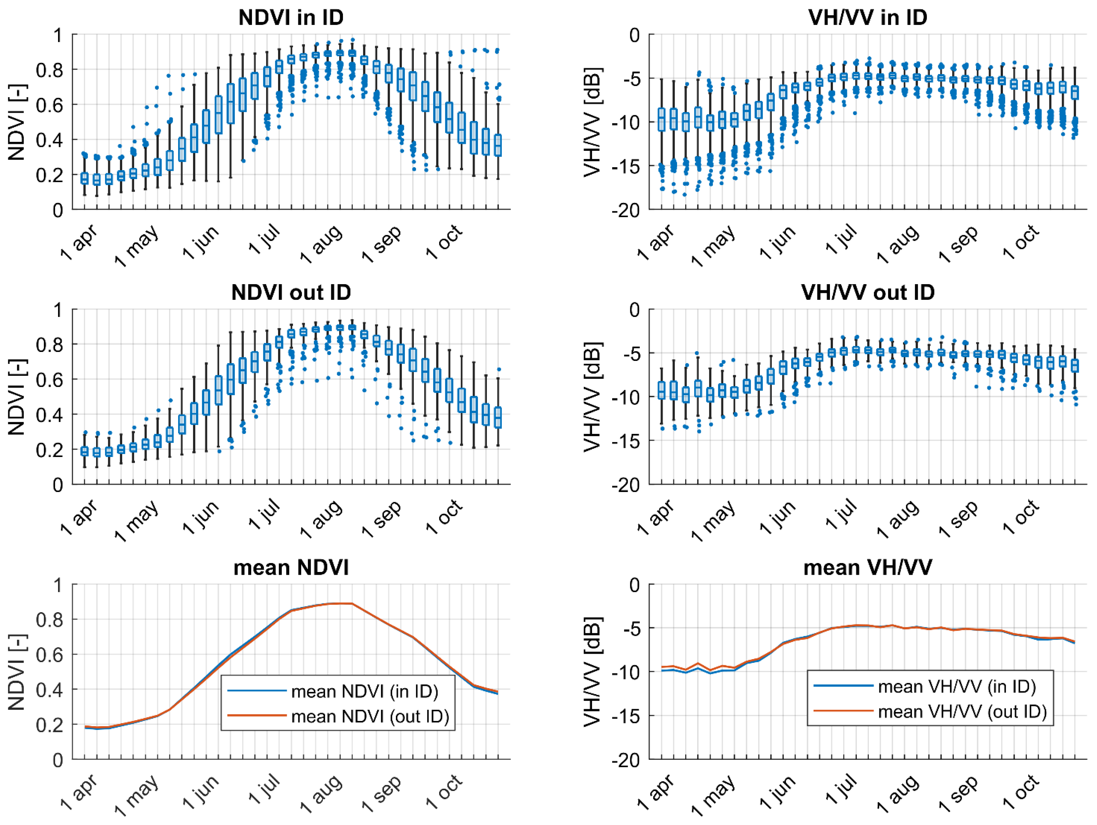
Figure 4.
Comparison of daily NDVI and daily Polarized Ratio Index (IPR) over maize fields, for different growing stages. (a): May–June–July period; (b): August–September–October period. Each point represents the comparison between daily NDVI and IPR for a specific field. During the middle and final phases, plants have reached the maximum stage of development (NDVI variability is very low and mainly due to plant health status) and the crop response in terms of NDVI is due to the change of plant color and to the final harvesting.
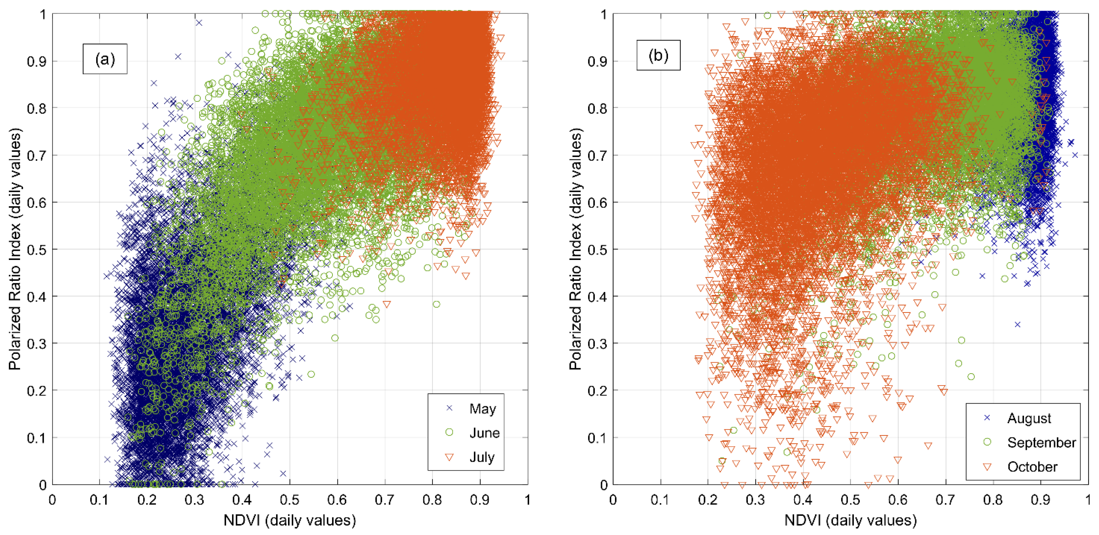
Figure 5.
Comparison of radar backscattering mean and variance during the initial period of maize growth. Each point represents a maize field during the period from May to June, colored according to the mean NDVI for the same period.
Figure 5.
Comparison of radar backscattering mean and variance during the initial period of maize growth. Each point represents a maize field during the period from May to June, colored according to the mean NDVI for the same period.
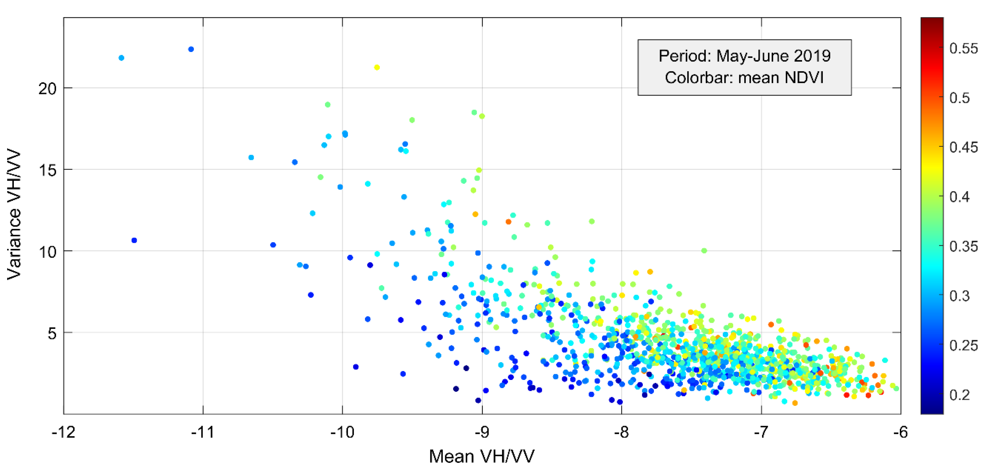
Figure 6.
(a) Temporal distribution of emergence periods (i.e., the periods when the plants emerge through the soil). The 6–days revised time refers to the availability of radar data that were used for the analysis. For each day, the hectares where the plants have come out from the ground have been cumulated according to the class of elevation (meters above the sea level). (b) Temporal variation of the frequency distribution. After the end of June, no more fields show values < 0.1, showing that the maize has passed the emergence phase.
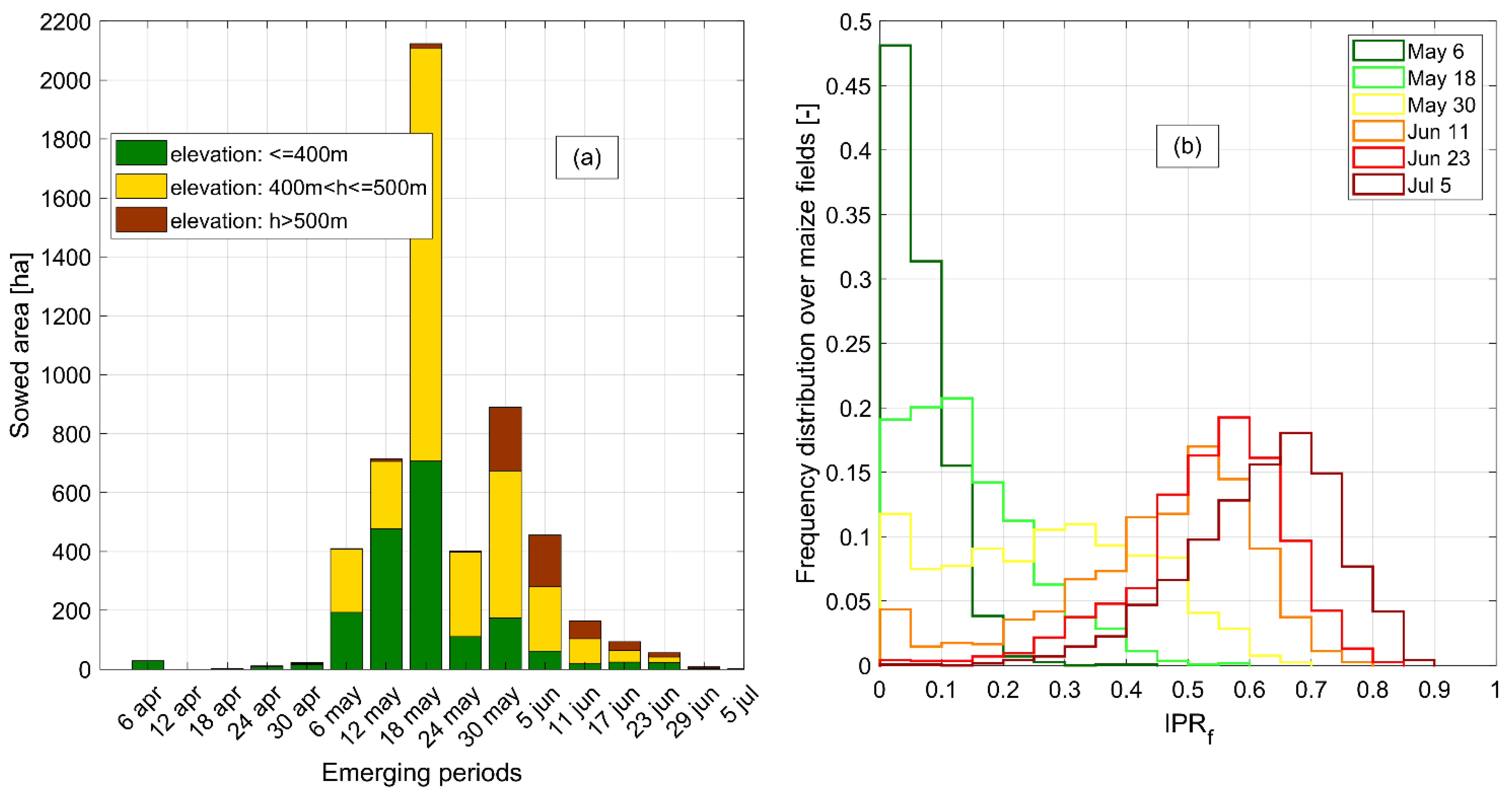
Figure 7.
Spatial distribution of sowing dates at 10 m × 10 m resolution. The sowing periods are grouped by 6-days classes. The spatial variability confirms the SAR analysis of emergence periods: for lower elevations, maize is sowed earlier on average.
Figure 7.
Spatial distribution of sowing dates at 10 m × 10 m resolution. The sowing periods are grouped by 6-days classes. The spatial variability confirms the SAR analysis of emergence periods: for lower elevations, maize is sowed earlier on average.

Table 1.
Columns 2–3 Pearson correlation coefficients (R) between NDVI and VH/VV. For each month from April to July, the optical and radar responses were compared, considering all the maize fields and a 6–days frequency. R was calculated for the group of fields within and outside the irrigation districts (ID). Columns 4–7 comparison between mean monthly NDVI [–] and soil moisture [Volwater/Volsoil] for the fields within and outside the irrigation districts (soil moisture refers to the soil upper layer: 3–5 cm).
| Month | Correlation between NDVI and VH/VV | Comparison of NDVI and Soil Moisture (SM) | ||||
|---|---|---|---|---|---|---|
| R (in ID) | R (out ID) | NDVI (in ID) | NDVI (out ID) | SM (in ID) | SM (out ID) | |
| April | 0.2 | 0.2 | 0.21 | 0.22 | 0.24 | 0.26 |
| May | 0.62 | 0.6 | 0.46 | 0.45 | 0.22 | 0.23 |
| June | 0.64 | 0.66 | 0.71 | 0.68 | 0.2 | 0.2 |
| July | 0.23 | 0.21 | 0.84 | 0.83 | 0.17 | 0.18 |
Publisher’s Note: MDPI stays neutral with regard to jurisdictional claims in published maps and institutional affiliations. |
© 2022 by the authors. Licensee MDPI, Basel, Switzerland. This article is an open access article distributed under the terms and conditions of the Creative Commons Attribution (CC BY) license (https://creativecommons.org/licenses/by/4.0/).
Share and Cite
MDPI and ACS Style
Rolle, M.; Tamea, S.; Claps, P.; Ayari, E.; Baghdadi, N.; Zribi, M. Analysis of Maize Sowing Periods and Cycle Phases Using Sentinel 1&2 Data Synergy. Remote Sens. 2022, 14, 3712. https://doi.org/10.3390/rs14153712
AMA Style
Rolle M, Tamea S, Claps P, Ayari E, Baghdadi N, Zribi M. Analysis of Maize Sowing Periods and Cycle Phases Using Sentinel 1&2 Data Synergy. Remote Sensing. 2022; 14(15):3712. https://doi.org/10.3390/rs14153712
Chicago/Turabian StyleRolle, Matteo, Stefania Tamea, Pierluigi Claps, Emna Ayari, Nicolas Baghdadi, and Mehrez Zribi. 2022. "Analysis of Maize Sowing Periods and Cycle Phases Using Sentinel 1&2 Data Synergy" Remote Sensing 14, no. 15: 3712. https://doi.org/10.3390/rs14153712
Note that from the first issue of 2016, this journal uses article numbers instead of page numbers. See further details here.