
Real-Time Software for the Efficient Generation of the Clumping Index and Its Application Based on the Google Earth Engine


1
Key Laboratory of Resources and Environmental Information System (LREIS), Institute of Geographic Sciences and Natural Resources Research, Chinese Academy of Sciences, Beijing 100101, China
2
University of Chinese Academy of Sciences, Beijing 100049, China
*
Author to whom correspondence should be addressed.
Remote Sens. 2022, 14(15), 3837; https://doi.org/10.3390/rs14153837
Submission received: 10 June 2022
/
Revised: 15 July 2022
/
Accepted: 3 August 2022
/
Published: 8 August 2022
(This article belongs to the Collection Google Earth Engine Applications)
Abstract
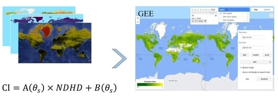
:Canopy clumping index (CI) is a key structural parameter related to vegetation phenology and the absorption of radiation, and it is usually retrieved from remote sensing data based on an empirical relationship with the Normalized Difference between Hotspot and Darkspot (NDHD) index. A rapid production software was developed to implement the CI algorithm based on the Google Earth Engine (GEE) to update current CI products and promote the application of CI in different fields. Daily, monthly, and yearly global CI products are continuously generated and updated in real-time by the software. Users can directly download the product or work with CI without paying attention to data generation. For the application case study, a change detection algorithm, LandTrendr, was implemented on the GEE to examine the global CI trend from 2000 to 2020. The results indicate that the area of increase trend (28.7%, ΔCI > 0.02) is greater than that of the decrease trend (17.1%, ΔCI < −0.02). Our work contributes toward the retrieval, application, and validation of CI.
1. Introduction
The canopy clumping index (CI) is a measurement of the spatial distribution pattern of foliage. Foliage commonly has a non-random distribution, which is aggregated at the canopy, branch, and shoot scales [1,2]. Theoretically, CI is >0. When CI < 1, the foliage has a clumping distribution. When CI > 1, the foliage has a regular distribution. The foliage has a random distribution when CI = 1. CI reflects the gap distribution within a vegetation canopy, thereby influencing light interception and evapotranspiration [3,4]. Previous studies have shown that the retrieval of other important vegetation indexes and the modeling of radiative transfer can be improved when the vegetation-clumping effect is taken into consideration [5,6,7]. Terrestrial ecological models also require CI as a key parameter for the better estimation of other variables, such as the Boreal Ecosystem Productivity Simulator [8], the soil temperature inversion procedure [9], and the canopy photosynthesis and evaporation model [10].
Currently, field and remote sensing methods are used to acquire CI [6]. The field method is categorized into direct and indirect methods. The direct method acquires CI by its straightforward definition as the ratio of effective leaf-area index to the leaf-area index [2,11,12]. The indirect method acquires CI using a series of optical instruments, such as digital hemispherical photography, the LAI-2200 plant canopy analyzer, and the tracing radiation and architecture of canopies, to manually capture the radiation above or below the canopy [6,13]. The field method is labor-intensive, and the obtained CI is limited to several plots wherein the model or relationship needs to be validated. The remote sensing method consists of the passive optical method, which is an estimation based on an empirical relationship between CI and indices constructed on reflectance values obtained from optical sensors [14,15]. The active light detection and ranging (LiDAR) method estimates CI using a gap-fraction-based method or a gap-size-based method using LiDAR cloud points because the laser pulse can penetrate the canopy [16,17].
Researchers have produced global CI products that are derived from optical images and process them locally. The spatial and temporal resolutions of these products range from 500 m to 6 km and daily to yearly, respectively [6,14,18,19,20]. In a previous study, we generated global and long-term coverage (2001–2017) of CI products (hereafter referred to as CAS-CI) with a high temporal resolution based on an empirical relationship between the Normalized Difference between the Hotspot and Darkspot (NDHD) reflectance values derived from the moderate resolution imaging spectroradiometer (MODIS) dataset [18]. The product is freely available (http://www.geodata.cn/thematicView/modisCI.html accessed on 25 May 2022), and it has been supporting a series of research projects. However, producing the global CI requires intensive computing due to the large quantity of input data and the enormous image preprocessing, and it utilizes complex algorithms. Additionally, the current CI products are faced with difficulties such as inefficient data distribution and limitations in terms of computation and storage, especially on a global scale. These disadvantages restrict the timely updating of global products, and thus impede research on and applications of CI. Similarly, these obstacles also exist in CAS-CI products as they are not scaled correctly, and their distribution to the global scale leads to heavy data downloading, which wastes storage and increases the cost of computation during subsequent data analysis. Although CAS-CI has a long-term time series, its increasing application demands the update of the temporal coverage of the current product and an efficient dissemination method. Remote sensing images are spatiotemporally collected on a continuous basis, which necessitates the researcher to frequently update CI, which involves a tremendous effort to maintain previous works by downloading locally to process numerous images. Therefore, it is desirable to automatically fetch ongoing satellite observations and disseminate CI products universally for immediate applications.
A cloud computing platform equipped with high computational and data storage capacities will enable one to overcome the above-mentioned difficulties. Rapid computation services provided via the internet facilitate a variety of applications involving complex modeling and the analysis of large amounts of data [21,22,23]. The Google Earth Engine (GEE) is a cloud-based platform that integrates online computation with extensive earth observation datasets (https://earthengine.google.org/ accesed on 25 May 2022). The GEE also consists of tools with specialized processing and visualization application programming interfaces for geospatial data. The GEE provides free personal storage of 250 Gbit to each account, allowing users to expediently carry out research using their own data, together with its continuously archived satellite images and released data products [24]. The GEE enables the convenient performance of large-scale and long-term geospatial analysis by way of computation offloading and allows users to visualize and export results. Many widely used algorithms are deployed on the GEE, thereby enabling the successful implementation of a series of thematic methods such as land cover mapping, vegetation index retrieval, and change detection algorithms [25,26,27]. Thematic software that is specifically designed for different applications is also deployed on GEE. For example, GEE-enabled software is provided for processing Landsat images such that they can be converted into a collection of spatiotemporally high-quality Landsat images [28], and other software is used for the rapid analysis of floodwater data to estimate the floodwater’s depth [29].
Consequently, our objective is to provide online software that completely leverages the strengths of image analysis and data synchronization in the GEE for the production of CI and its visualization and custom download, which enables fast utilization of the CI product and the quick receipt of feedback to improve future CI estimation. This GEE-embedded software was developed to produce CI products in line with the methods and technologies that are available in some previous works [15,18]. Additionally, a change detection algorithm, namely, Landsat-based detection of trends in disturbance and recovery (LandTrendr), was implemented directly on the GEE to examine the characteristics of changes in global CI as a test case and track the temporal change of yearly CI during 2000–2020.
2. Retrieval Software Design
2.1. Materials
The input to the software is provided by the MODIS image datasets archived in the GEE and other required datasets that were not included in the GEE, such as the fraction of vegetation cover (fCover) and global land-cover classification product (GLC2000) (Table 1). Kernel parameters such as ,, and (MCD43A1) and observation information including MOD09A1 and MYD09A1 are MODIS-released products that are already archived in GEE. The normalized difference vegetation index (NDVI) as an input was calculated from the near-infrared band and the red band products from MCD43A4. MCD43A2 records the degree of contamination in pixels during the imaging process, which was used to indicate the quality of the final product. The GEOV fCover V2 was used as the input, and it was comprised of a collection with a 4-month interval that was released every 10 days. The fCover was uploaded into the GEE using monthly images, with the earliest start date of each month from March 2000 to May 2020. GLC2000 mapped the relatively detailed global vegetation categories, and it was also manually uploaded as a single image. All datasets can be filtered by the date specified by users, and the filtered image collection is sliced daily by matching their temporal resolution and then used in the software.
2.2. CI Retrieval Method
Optical remote sensing data are commonly used to estimate CI products by building an empirical relationship with reflectance or the vegetation index [6,14]. The retrieval algorithm adopted by Wei et al. [18] uses the linear relationship between CI and NDHD (Figure 1):
where is the solar zenith angle (SZA), and are coefficients jointly determined by solar zenith and the shape of the vegetation canopy, previously modelled by Chen et al. [14]. The NDHD can be calculated using Equation (2)
where and denote the reflectance at the hotspot and darkspot directions, respectively. The Ross–Li model [30,31] is used to calculate and :
where are the solar zenith, observational, and relative azimuth angles, respectively. was calculated when equaled and was set to 0. was derived when equaled and was set to 180°.
The SZA is an average value between Terra and Aqua overpasses in their overlapping date obtained from observation information described in Section 2.1. ,, and are kernel parameters provided by the red band of MODIS43A1 products. and are parts of the bidirectional reflectance distribution function (BRDF) [30]. The expression to compute is based on Roujean et al. [32].
is called the LiSparse-R kernel, which is derived from Li et al. [33]. The expression and parameter settings are as follows:
The variables and are theoretically in the range of 0–90° was set to 0° or 180° for the calculation of reflectance corresponding to the hotspot and darkspot, respectively. The dimensionless parameters and were preselected from [30]. was set to 60° when the fCover was <25%, to reduce the overestimation of CI in sparsely vegetated areas.
Finally, the hotspot correction was conducted through an empirical relationship between the Ross–Li derived MODIS and the polarization and directionality of the Earth reflectance (POLDER) hotspots:
is the difference in reflectance between POLDER and MODIS hotspots, to be parameterized by NDVI and for the red band of MODIS BRDF.
2.3. Software Design
To ensure the consistency of the computed CI by the developed software with that of the initial version of the products, the retrieval process followed the previous method by Wei et al. [18], in which a lookup table was built between the hotspot/darkspot value and the observation information was matched according to the input. This software directly computes CI instead of matching based on criteria because computation at a global scale is not worth considering in the GEE.
The general steps for retrieval are listed briefly as follows:
Step 1: Filter dataset by the user designated the date for new image collections.
Step 2: Select bands needed to be calculated using image collections to generate multi-band images for each day.
Step 3: The daily CI was retrieved based on band calculations, and low-quality pixels were excluded.
Step 4: The Savitzky–Golay smoothing filter (SG-filter) [34] was applied for daily CI collection, and then the monthly or yearly CI image was composited using quality indicators to provide the final CI for download.
When calculating NDHD, and were confined to the range of 0–60° at an increment of 10° and the pixels with an observation angle of >60° or their corresponding fCover of <0.25 were set to 60°. Therefore, and can also be calculated in advance based on the three parameters of angle and Equations (4)–(6) (Table 2). During the determination of the final linear coefficients (A and B), and were confined to an increment of 5°.
The quality and snow bands of MCD43A2 were used to exclude the contaminated pixels and indicate the retrieval quality of CI pixels, and based on the quality, the quality indicator band (QA) was generated and integrated into the final export. The main (QA = 0) and magnitude (QA = 2) inversions indicate the higher and lower qualities of CI, respectively. The generation of the QA was done according to Wei et al. [18]. For compositing, all the main inversions of the CI results within a month or year were selected based on quality information, and then their averages were computed and mosaiced with the average of the magnitude inversions to generate high-quality monthly or yearly CI images. Some settings of the final images for downloading are listed in Table 3.
For convenience, a multiple band image was first generated by selecting corresponding bands from each remote sensing dataset at a given interval. The most recent image was repeatedly used when these datasets had no available image due to the difference in temporal resolution between remote sensing datasets, which proves that the retrieval of daily CI is possible. After all daily images consisting of input bands were ready, CI retrieval was conducted on a global scale. Software was devoted to provide a user-friendly interface to allow users to select the date and spatial coverage to export required products.
3. Results
3.1. GEE-Based Software to Retrieve and Download CI
The software developed for GEE’s JavaScript version mainly provides an online function of “generation and then download” for CI. The initial interface of this software is shown in Figure 2.
After inputting the two dates (period) formatted as date strings, one of the buttons with text as daily, monthly, and yearly is clicked. The next screen will show the corresponding date list for selection. The daily CI image will be directly generated after smoothing. The monthly and yearly CI images are averaged from the daily smoothed CIs within the selected month and year, respectively. This software allows users to download the CI product via real-time online generation by a self-defined date and coverage, which is an improvement over the initially released product that preserves locally first and then provides for global download. The product containing CI and quality information is exported in the GeoTIFF format to the Google drive that shares the same account with that of the GEE. The image value is scaled by 1000 times to achieve a compact file size. The product can also be directly exported with only a part of the image by selecting only a small region to download. Because of constraints in the GEE, while exporting the global extent (60°S–90°N and 180°E–180°W), the product will be automatically clipped into nine equal-sized parts of the image.
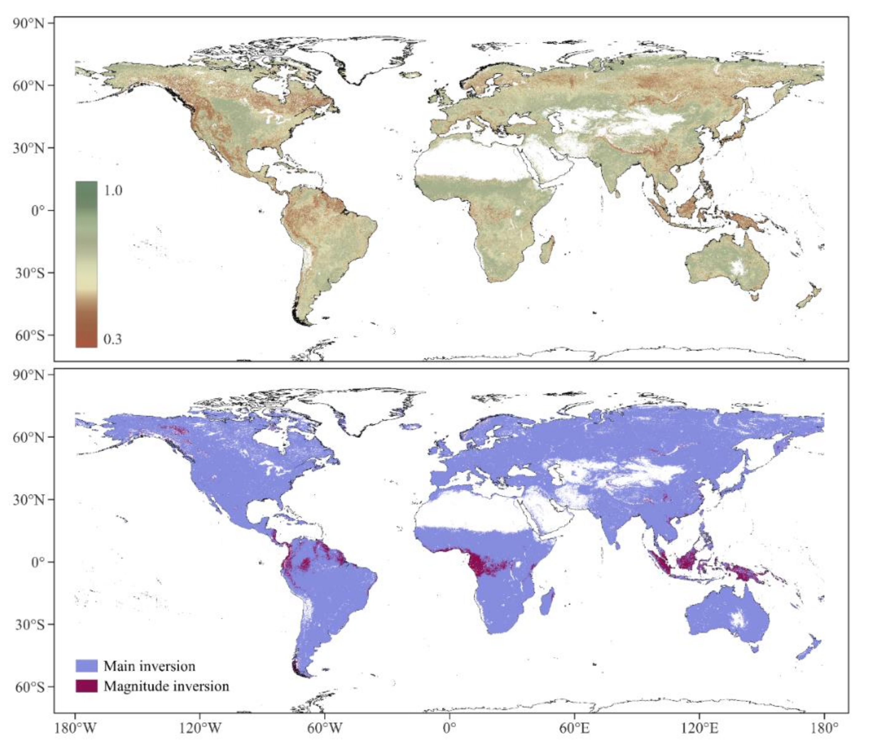
Figure 3 displays the global CI in 2020, and its quality distribution was computed by this software. The lower CI is concentrated in the forest region, e.g., the equatorial regions and boreal forest. The higher CI is primarily observed in arid or semiarid regions. The magnitude inversion is observed in South America, Central Africa, and Southeast Asia because of the continuous cloud cover over these areas. The results derived from this online retrieval software are very consistent with those of Wei et al. [18]. Additionally, the average CI in January, April, July, and October from 2000 to 2020 was composited using this software and exported to display the seasonal variation of CI (Figure 4). In the Northern Hemisphere, the CI reaches the maximum in January, and the valid CI areas are relatively small because of low vegetation coverage in winter. In July, a low CI is observed in eastern Eurasia and North America. In the equatorial region, the CI is always low because of dense forest coverage.
3.2. Temporal Variation of CI
Variations in CI reflect specific temporal characteristics of vegetation growth, disturbances, and radiation budget and may indicate climate change in terms of long-term ecological dynamics [35,36]. Change detection in global CI can provide a rich and temporally consistent description for the trend, the change magnitude, and the date of change. A change detection algorithm (LandTrendr) was implemented for the time series of annual average CI as a test case to find the change trend. LandTrendr first segments the entire series from 2000 to 2020 into several segments based on the statistic method. Each segment indicates the monotonously increased, decreased, or stable trend in a specific period. In this study, the trend segment with the maximum change magnitude was selected to analyze and remove trend segments that covered <3 years because several segments can be detected from the time series of CI.
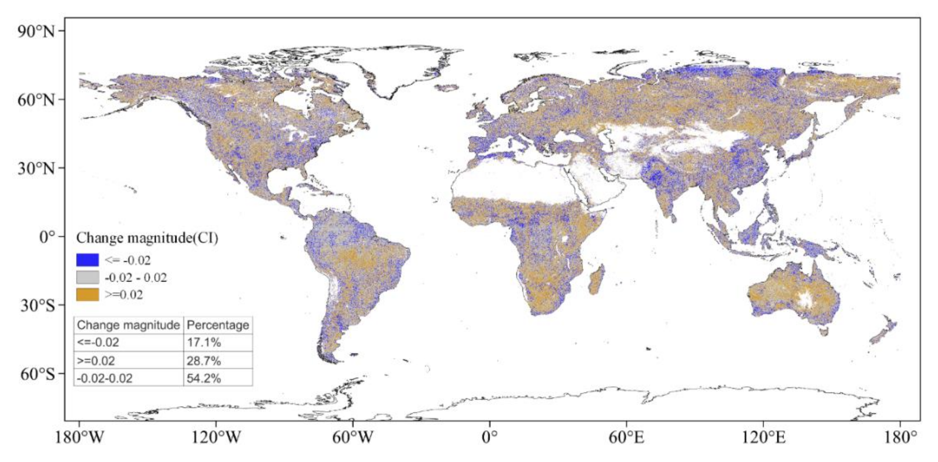
The CI change magnitude (Figure 5) was derived from the difference between the two CI values, corresponding to the start and end dates of the trend. The results indicate that 54.2% of the pixels have no abrupt or gradual trend in the entire time series, and 28.7% of the pixels show a positive trend. A negative trend (17.1%) indicates that the foliage of vegetation is clumping, and this situation is mainly distributed in evergreen forests. The decreasing trend was tracked in northern India and central China, which is consistent with the results of Wei et al. [18].
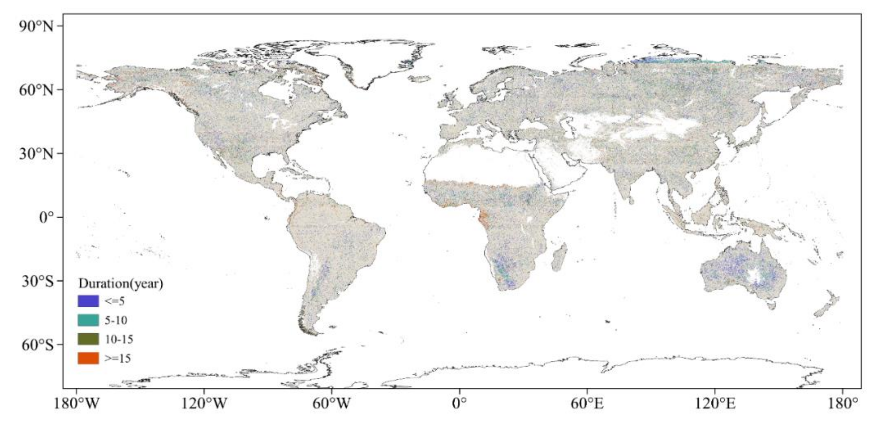
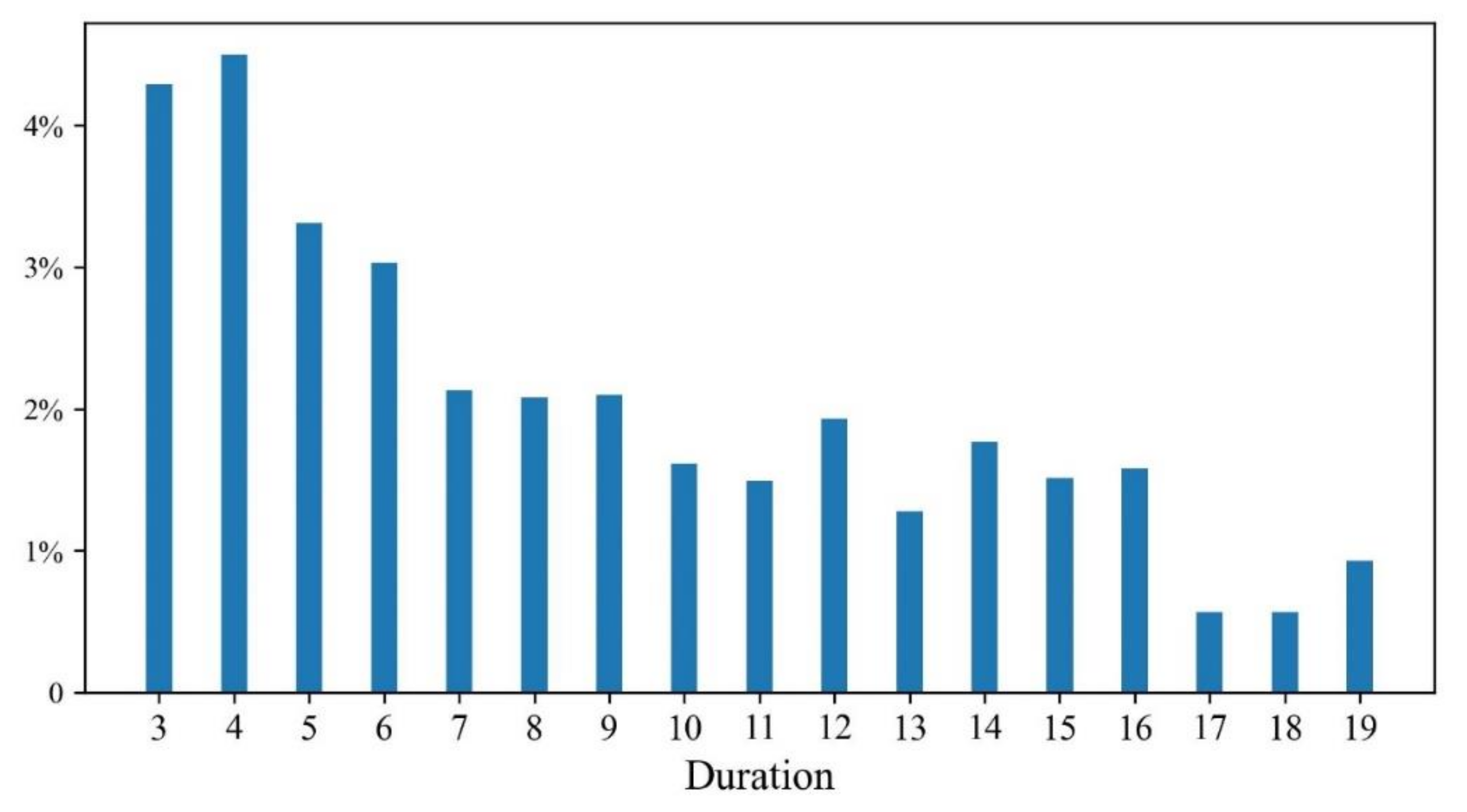
Because the annual variation of CI is not distinct compared to its seasonal variation [20], the annual average value can cover the difference that exists in the specific period. Additionally, the range of CI is from 0.3 to 1.0, and its trajectories do not show variation as significantly as the LAIs [15,19]; therefore, the marginal trend is inadequate for detection by the LandTrendr. Here, for better comparison, the spatial distribution of duration and its percentage were drawn except for the 21-year segment (full-period trend) as most of the area exhibited a stable trend during the 21 years. Figure 6 spatially displays the duration of the segment trend through discrete coloring for 5-year intervals, and Figure 7 shows the statistics for the duration. These illustrate that the segment trend was maintained for a few years; however, the trend persisted for the full period, and those segments tended to concentrate in arid regions or those of very high latitude. The successive distribution of several year-long segments in those areas could have been induced by the bad retrieval of CI or the occurrence of strong disturbance of the vegetation.
4. Discussion
4.1. Contribution of the Study
For the design of the CI retrieval software, many types of data, including the monthly fraction of vegetation coverage and the landcover map, were first uploaded to the GEE and then shared publicly so that others can directly obtain results using this visualization software. Our software generates and disseminates canopy CI effectively and conveniently and thus supports subsequent research to be conducted efficiently within a user-defined scale. First, our CI retrieval software runs on the internet, without installation and extra requirements for personal computation, and directly provides downloading of CI at three temporal scales (daily, monthly, and yearly). In terms of retrieval, the CI was smoothed using an SG-filter for the user-selected collection to ensure spatiotemporal consistency and continuity, which is otherwise inhibited due to the difference in satellite observation quality at different time points. The monthly or yearly export is averaged from the smoothed collection and then composited. A comparison of the offline and GEE outputs was added to Appendix A. The year 2019 was selected for the comparison. The two outputs show consistent fluctuation (Figure A1). The GEE output shows more distinct seasonal variation but slightly underestimates the offline CI (bias <0.03). This is mainly attributed to a new version of fCover used in the GEE estimation. The GEE version uses the NDHD method directly, while the offline estimation retrieves multiple values first from the lookup table and outputs the averaged value.
Three different kinds of temporal-scale CI products with their quality indicators for the period March 2000 to May 2020 were released using this software. Users can also define their spatial or temporal scale to obtain CI products through a very simple modification of relative parameters in the shared code. fCover will be continually uploaded once the latest is updated on https://land.copernicus.vgt.vito.be/ (accesed on 25 May 2022) to enable our software to generate a real-time CI product as soon as the MODIS products are renewed in the GEE. Consequently, the developed CI downloading software with its code extends current product coverage and provides an opportunity to update CI products at the same pace at which data are input.
4.2. Applicability of the Software
A variety of key variables related to the ecological function of vegetation are influenced by the foliage clumping effect [3,12,37]. Our software is very promising as it is integrated with the global CI product to estimate global products such as vegetation cover, leaf-area index, and evapotranspiration. The GEE provides a series of basic operations for image or other geospatial data, together with thematic algorithms such as classification, deep learning, and change detection. Therefore, this software provides the possibility to conduct global-scale research related to CI relying on abundant remote sensing data archived in the GEE and its powerful computation ability. Consequently, we recommend that a large-scale analysis related to CI can be directly conducted on the GEE because it supports better online data-intensive processing than downloading data of several decades.
The variation in CI indicates the change in vegetation in terms of phenology, the receipt of radiation, and growth trends during ecological processes. The test case shows that the annual averaged CI has a relatively stable trend from 2000 to 2020, and this could be because of the relatively distinct variation in seasonal CI instead of the interannual average CI. The key characteristics derived from the change detection in seasonal CI have promising applications in terms of classification of vegetation, phenology monitoring, and climate change modeling.
4.3. Retrieval of CI in the GEE
The new version of monthly fCover was adopted in the production period. The fCover with a spatial resolution of 1 km was produced based on SPOT/VEGETATION data; however, it was not archived by the GEE [38]. Currently, the spatial matching fCover was produced based on a linear analysis of spectral reflectance derived from MODIS [39], which could be easily implemented in the GEE. The uploaded GLC2000 is a single image that determines the final retrieval coefficients based on the vegetation type. The global MODIS yearly land cover product was archived in the GEE. Therefore, all required data for CI retrieval were directly provided or further generated using the MODIS observation dataset. Additionally, the MODIS dataset has been continuously collected and accumulated in the GEE, which enables one to achieve a better spatiotemporally matched CI retrieval by avoiding a manual upload of the required data.
The CI retrieval by this software was achieved based on the generation of a look up table, indicating that the CI result is an approximation because input data were approximated. Therefore, the new retrieval algorithm is expected to directly link the input and output.
5. Conclusions
The increasing requirements for global CI pose significant challenges for data processing, storage, and dissemination. Current CI products need continuous updating to deal with the continuous generation of new data. To alleviate restrictions posed by previous products and make the application of CI convenient, visualization software that actualizes CI retrieval was developed by relying on the GEE to allow users to download and use real-time products that can be customized based on specific regions and dates. The CI is an important structural parameter of vegetation that influences the transfer of radiation by interacting with the canopy. Based on the developed software, global-scale research on CI can be directly carried out under the aegis of the GEE. The developed software will continuously update CI as soon as the latest materials are available in the GEE. Our retrieval program, which is coded using JavaScript, is shared such that many research contributions to and applications of CI can be achieved globally.
Author Contributions
Conceptualization, Y.L. and H.F.; software, Y.L.; writing—original draft preparation, Y.L.; and writing—review and editing, Y.L. and H.F. All authors have read and agreed to the published version of the manuscript.
Funding
This study was partly supported by a grant from State Key Laboratory of Resources and Environmental Information System.
Acknowledgments
The authors would like to thank Shanshan Wei and Yinghui Zhang for their support regarding the implementation of the algorithm, and Sijia Li and Miao Yu for their assistance with the software testing. We also thank the developers in the GEE community for sharing very useful sample codes.
Conflicts of Interest
The authors declare no conflict of interest.
Code Availability
JavaScript code can be found from: (1) https://code.earthengine.google.com/?scriptPath=uers%2Flrvings%2FGMap%3AClumpingIndex%2FCAS-CI (accesed on 12 January 2022); (2) https://github.com/CUGLiving/CAS-Clumping-Index-Products (accesed on 12 January 2022).
Appendix A
A comparison of CI derived from GEE with the offline CAS-CI product.
Figure A1.
Comparisons of the CI time series derived from GEE and the CAS-CI (8-day, 2019).

References
- Chen, J.M.; Black, T.A. Foliage area and architecture of plant canopies from sunfleck size distributions. Agric. For. Meteorol. 1992, 60, 249–266. [Google Scholar] [CrossRef]
- Nilson, T. A theoretical analysis of the frequency of gaps in plant stands. Agric. Meteorol. 1971, 8, 25–38. [Google Scholar] [CrossRef]
- Chen, B.; Lu, X.; Wang, S.; Chen, J.M.; Liu, Y.; Fang, H.; Liu, Z.; Jiang, F.; Arain, M.A.; Chen, J.; et al. Evaluation of clumping effects on the estimation of global terrestrial evapotranspiration. Remote Sens. 2021, 13, 4075. [Google Scholar] [CrossRef]
- Law, B.E.; Cescatti, A.; Baldocchi, D.D. Leaf area distribution and radiative transfer in open-canopy forests: Implications for mass and energy exchange. Tree Physiol. 2001, 21, 777–787. [Google Scholar] [CrossRef] [Green Version]
- Zhao, J.; Li, J.; Liu, Q.; Xu, B.; Yu, W.; Lin, S.; Hu, Z. Estimating fractional vegetation cover from leaf area index and clumping index based on the gap probability theory. Int. J. Appl. Earth Obs. Geoinf. 2020, 90, 102112. [Google Scholar] [CrossRef]
- Fang, H. Canopy clumping index (CI): A review of methods, characteristics, and applications. Agric. For. Meteorol. 2021, 303, 108374. [Google Scholar] [CrossRef]
- Ni-Meister, W.; Yang, W.; Kiang, N.Y. A clumped-foliage canopy radiative transfer model for a global dynamic terrestrial ecosystem model. I: Theory. Agric. For. Meteorol. 2010, 150, 881–894. [Google Scholar] [CrossRef]
- Chen, J.M.; Mo, G.; Pisek, J.; Liu, J.; Deng, F.; Ishizawa, M.; Chan, D. Effects of foliage clumping on the estimation of global terrestrial gross primary productivity. Glob. Biogeochem. Cycles 2012, 26, GB1019. [Google Scholar] [CrossRef]
- Bian, Z.; Cao, B.; Li, H.; Du, Y.; Song, L.; Fan, W.; Xiao, Q.; Liu, Q. A robust inversion algorithm for surface leaf and soil temperatures using the vegetation clumping index. Remote Sens. 2017, 9, 780. [Google Scholar] [CrossRef] [Green Version]
- Baldocchi, D.D.; Harley, P.C. Scaling carbon dioxide and water vapour exchange from leaf to canopy in a deciduous forest. II. Model testing and application. Plant Cell Environ. 1995, 18, 1157–1173. [Google Scholar] [CrossRef]
- Chen, J.M. 3.06-remote sensing emote sensing of leaf area index and clumping index. In Comprehensive Remote Sensing; Liang, S., Ed.; Elsevier: Oxford, UK, 2018; pp. 53–77. [Google Scholar]
- Fang, H.; Baret, F.; Plummer, S.; Schaepman-Strub, G. An overview of global leaf area index (LAI): Methods, products, validation, and applications. Rev. Geophys. 2019, 57, 739–799. [Google Scholar] [CrossRef]
- Braghiere, R.K.; Quaife, T.; Black, E.; Ryu, Y.; Chen, Q.; De Kauwe, M.G.; Baldocchi, D. Influence of sun zenith angle on canopy clumping and the resulting impacts on photosynthesis. Agric. For. Meteorol. 2020, 291, 108065. [Google Scholar] [CrossRef]
- Chen, J.M.; Menges, C.H.; Leblanc, S.G. Global mapping of foliage clumping index using multi-angular satellite data. Remote Sens. Environ. 2005, 97, 447–457. [Google Scholar] [CrossRef]
- Wei, S.; Fang, H. Estimation of canopy clumping index from MISR and MODIS sensors using the normalized difference hotspot and darkspot (NDHD) method: The influence of BRDF models and solar zenith angle. Remote Sens. Environ. 2016, 187, 476–491. [Google Scholar] [CrossRef]
- Wang, Y.; Fang, H.L. Estimation of LAI with the LiDAR technology: A review. Remote Sens. 2020, 12, 3457. [Google Scholar] [CrossRef]
- Wilson, J.W. Stand structure and light penetration. I. Analysis by point quadrats. J. Appl. Ecol. 1965, 2, 383–390. [Google Scholar] [CrossRef]
- Wei, S.; Fang, H.; Schaaf, C.B.; He, L.; Chen, J.M. Global 500 m clumping index product derived from MODIS BRDF data (2001–2017). Remote Sens. Environ. 2019, 232, 111296. [Google Scholar] [CrossRef]
- He, L.; Chen, J.M.; Pisek, J.; Schaaf, C.B.; Strahler, A.H. Global clumping index map derived from the MODIS BRDF product. Remote Sens. Environ. 2012, 119, 118–130. [Google Scholar] [CrossRef]
- Jiao, Z.; Dong, Y.; Schaaf, C.B.; Chen, J.M.; Román, M.; Wang, Z.; Zhang, H.; Ding, A.; Erb, A.; Hill, M.J.; et al. An algorithm for the retrieval of the clumping index (CI) from the MODIS BRDF product using an adjusted version of the kernel-driven BRDF model. Remote Sens. Environ. 2018, 209, 594–611. [Google Scholar] [CrossRef]
- Kennedy, R.E.; Yang, Z.; Cohen, W.B. Detecting trends in forest disturbance and recovery using yearly Landsat time series: 1. LandTrendr—Temporal segmentation algorithms. Remote Sens. Environ. 2010, 114, 2897–2910. [Google Scholar] [CrossRef]
- Hua, G.-J.; Hung, C.-L.; Tang, C.Y.; Lin, Y.-L. Cloud computing service framework for bioinformatics tools. In Proceedings of the IEEE International Conference on Bioinformatics and Biomedicine-Medical Informatics and Decision Making, Washington, DC, USA, 9–12 November 2015; pp. 1509–1513. [Google Scholar]
- Li, X.Y.; Wang, H.; Wang, X.N.; Zhang, W.; Tang, Y.L. The application analysis of cloud computation technology into electronic information system. In Proceedings of the International Conference on Mechatronics Engineering and Computing Technology (ICMECT), Shanghai, China, 9–10 April 2014; pp. 5552–5555. [Google Scholar]
- Gorelick, N.; Hancher, M.; Dixon, M.; Ilyushchenko, S.; Thau, D.; Moore, R. Google earth engine: Planetary-scale geospatial analysis for everyone. Remote Sens. Environ. 2017, 202, 18–27. [Google Scholar] [CrossRef]
- Li, Y.; Liu, M.; Liu, X.; Yang, W.; Wang, W. Characterising three decades of evolution of forest spatial pattern in a major coal-energy province in northern China using annual landsat time series. Int. J. Appl. Earth Obs. Geoinf. 2021, 95, 102254. [Google Scholar] [CrossRef]
- Dong, J.; Xiao, X.; Menarguez, M.A.; Zhang, G.; Qin, Y.; Thau, D.; Biradar, C.; Moore, B., 3rd. Mapping paddy rice planting area in northeastern Asia with Landsat 8 images, phenology-based algorithm and Google earth engine. Remote Sens. Environ. 2016, 185, 142–154. [Google Scholar] [CrossRef] [Green Version]
- Kennedy, R.; Yang, Z.; Gorelick, N.; Braaten, J.; Cavalcante, L.; Cohen, W.; Healey, S. Implementation of the LandTrendr algorithm on google earth engine. Remote Sens. 2018, 10, 691. [Google Scholar] [CrossRef] [Green Version]
- Li, H.; Wan, W.; Fang, Y.; Zhu, S.; Chen, X.; Liu, B.; Hong, Y. A Google earth engine-enabled software for efficiently generating high-quality user-ready landsat mosaic images. Environ. Model. Softw. 2019, 112, 16–22. [Google Scholar] [CrossRef]
- Peter, B.G.; Cohen, S.; Lucey, R.; Munasinghe, D.; Raney, A.; Brakenridge, G.R. Google earth engine implementation of the floodwater depth estimation tool (FwDET-GEE) for rapid and large scale flood analysis. IEEE Geosci. Remote Sens. Lett. 2022, 19, 1–5. [Google Scholar] [CrossRef]
- Lucht, W.; Schaaf, C.B.; Strahler, A.H. An algorithm for the retrieval of albedo from space using semiempirical BRDF models. IEEE Trans. Geosci. Remote Sens. 2000, 38, 977–998. [Google Scholar] [CrossRef] [Green Version]
- Wanner, W.; Li, X.; Strahler, A.H. On the derivation of kernels for kernel-driven models of bidirectional reflectance. J. Geophys. Res. Atmos. 1995, 100, 21077–21089. [Google Scholar] [CrossRef]
- Roujean, J.L.; Leroy, M.; Deschamps, P.Y. A bidirectional reflectance model of the Earth's surface for the correction of remote sensing data. J. Geophys. Res. Atmos. 1992, 97, 20455–20468. [Google Scholar] [CrossRef]
- Li, X.; Strahler, A.H. Geometric-optical bidirectional reflectance modeling of the discrete crown vegetation canopy: Effect of crown shape and mutual shadowing. IEEE Trans. Geosci. Remote Sens. 1992, 30, 276–292. [Google Scholar] [CrossRef]
- Savitzky, A.; Golay, M.J.E. Smoothing and differentiation of data by simplified least squares procedures. Anal. Chem. 1964, 36, 1627–1639. [Google Scholar] [CrossRef]
- Casella, E.; Sinoquet, H. Botanical determinants of foliage clumping and light interception in two-year-old coppice poplar canopies: Assessment from 3-D plant mock-ups. Ann. For. Sci. 2007, 64, 395–404. [Google Scholar] [CrossRef] [Green Version]
- Pisek, J.; Reznickova, L.; Adamson, K.; Ellsworth, D.S. Leaf inclination angle and foliage clumping in an evergreen broadleaf Eucalyptus forest under elevated atmospheric CO2. Aust. J. Bot. 2021, 69, 622–629. [Google Scholar] [CrossRef]
- Hill, M.J.; Román, M.O.; Schaaf, C.B.; Hutley, L.; Brannstrom, C.; Etter, A.; Hanan, N.P. Characterizing vegetation cover in global savannas with an annual foliage clumping index derived from the MODIS BRDF product. Remote Sens. Environ. 2011, 115, 2008–2024. [Google Scholar] [CrossRef]
- Verger, A.; Baret, F.; Weiss, M. Near real-time vegetation monitoring at global scale. IEEE J. Sel. Top. Appl. Earth Observ. Remote Sens. 2014, 7, 3473–3481. [Google Scholar] [CrossRef]
- Filipponi, F.; Valentini, E.; Nguyen Xuan, A.; Guerra, C.A.; Wolf, F.; Andrzejak, M.; Taramelli, A. Global MODIS fraction of green vegetation cover for monitoring abrupt and gradual vegetation changes. Remote Sens. 2018, 10, 653. [Google Scholar] [CrossRef] [Green Version]
Figure 1.
The procedure of the CI retrieval method based on the normalized difference between the hotspot and dark spot (NDHD) method. See Table 1 for a description of input data.
Figure 1.
The procedure of the CI retrieval method based on the normalized difference between the hotspot and dark spot (NDHD) method. See Table 1 for a description of input data.

Figure 2.
The graphic user interface for the CI retrieval and downloading tool. After the input of two dates, the corresponding selection appears. For detailed information on software usage, refer to https://github.com/CUGLiving/CAS-Clumping-Index-Products (accessed on 8 June 2022).
Figure 2.
The graphic user interface for the CI retrieval and downloading tool. After the input of two dates, the corresponding selection appears. For detailed information on software usage, refer to https://github.com/CUGLiving/CAS-Clumping-Index-Products (accessed on 8 June 2022).

Figure 3.
The global product composited from the daily product collection in 2020. The top panel shows the global CI distribution, and the quality indicator is discretely colored in the bottom panel.
Figure 3.
The global product composited from the daily product collection in 2020. The top panel shows the global CI distribution, and the quality indicator is discretely colored in the bottom panel.

Figure 4.
Global monthly CI in (a) January, (b) April, (c) July, and (d) October, aggregated from 2000 to 2020.
Figure 4.
Global monthly CI in (a) January, (b) April, (c) July, and (d) October, aggregated from 2000 to 2020.

Figure 5.
Change magnitude of CI between the two dates of the detected trend segment during the entire period (2000–2020). The attached table shows the percentage of number of pixels.
Figure 5.
Change magnitude of CI between the two dates of the detected trend segment during the entire period (2000–2020). The attached table shows the percentage of number of pixels.

Figure 6.
The spatial distribution of duration of the segmented change trends was discretely rendered at a 5-year interval. The unchanged area, together with the full-period segment of the trend, is shown in gray for better visualization.
Figure 6.
The spatial distribution of duration of the segmented change trends was discretely rendered at a 5-year interval. The unchanged area, together with the full-period segment of the trend, is shown in gray for better visualization.

Figure 7.
The percentage distribution of duration of the trend segment sustains. Note that the full-period trend segments were not included in this statistic.
Figure 7.
The percentage distribution of duration of the trend segment sustains. Note that the full-period trend segments were not included in this statistic.


Table 1.
Remote sensing data sets used in the CI retrieval. The column description lists the temporal and spatial resolutions of datasets. MODIS products have been archived in GEE; last two data were uploaded manually to the GEE.
Table 1.
Remote sensing data sets used in the CI retrieval. The column description lists the temporal and spatial resolutions of datasets. MODIS products have been archived in GEE; last two data were uploaded manually to the GEE.
| Name | Usage | Description | Available Site |
|---|---|---|---|
| MCD43A1.v6 | Red band BRDF coefficients ) | Daily, 500 m | Available in GEE |
| MCD43A2.v6 | Quality indicator of red band BRDF product | Daily, 500 m | Available in GEE |
| MCD43A4.v6 | Nadir BRDF-adjusted reflectance to derive NDVI | Daily, 500 m | Available in GEE |
| MOD09A1.v6 | SZA when Terra over pass | 8 days, 500 m | Available in GEE |
| MYD09A1.v6 | SZA when Aqua over pass | 8 days, 500 m | Available in GEE |
| GEOV fCover.v2 | Vegetation cover fraction to confine SZA | Monthly, 1 km | https://land.copernicus.vgt.vito.be/ (accessed on 12 January 2022) |
| GLC2000 landcover | Vegetation type for determination of coefficients (A,B) | Once, 1 km | https://forobs.jrc.ec.europa.eu/ (accessed on 12 January 2022) |
Table 2.
and , corresponding to hotspot ( and darkspot (, can be calculated against solar zenith angle (SZA) at an increment of 10°.
Table 2.
and , corresponding to hotspot ( and darkspot (, can be calculated against solar zenith angle (SZA) at an increment of 10°.
| , | ||||
| 0° | 0 | 0 | 0 | 0 |
| 10° | 0.0121 | −0.0288 | 0.0156 | −0.4552 |
| 20° | 0.0504 | −0.0876 | 0.0682 | −0.9125 |
| 30° | 0.1215 | −0.1342 | 0.1786 | −1.3094 |
| 40° | 0.2398 | −0.1228 | 0.3986 | −1.6108 |
| 50° | 0.4364 | 0.0042 | 0.8645 | −2.1114 |
| 60° | 0.7853 | 0.3424 | 1.9999 | −2.9999 |
Table 3.
Settings of the exported files. The quality indicator band (QA) records the quality of CI inversion.
Table 3.
Settings of the exported files. The quality indicator band (QA) records the quality of CI inversion.
| Image | Setting |
|---|---|
| Name | Named by corresponding date |
| Bands | Band 1:CI, band 2: QA (0: main inversion; 2: magnitude inversion; and 255: filled value) |
| Format | GeoTIFF |
| Scaled | Band 1: 1000; band2: none |
| Projection | WGS-84 |
| Spatial resolution | 500 m |
| File size | ~845 M (global image) |
Publisher’s Note: MDPI stays neutral with regard to jurisdictional claims in published maps and institutional affiliations. |
© 2022 by the authors. Licensee MDPI, Basel, Switzerland. This article is an open access article distributed under the terms and conditions of the Creative Commons Attribution (CC BY) license (https://creativecommons.org/licenses/by/4.0/).
Share and Cite
MDPI and ACS Style
Li, Y.; Fang, H. Real-Time Software for the Efficient Generation of the Clumping Index and Its Application Based on the Google Earth Engine. Remote Sens. 2022, 14, 3837. https://doi.org/10.3390/rs14153837
AMA Style
Li Y, Fang H. Real-Time Software for the Efficient Generation of the Clumping Index and Its Application Based on the Google Earth Engine. Remote Sensing. 2022; 14(15):3837. https://doi.org/10.3390/rs14153837
Chicago/Turabian StyleLi, Yu, and Hongliang Fang. 2022. "Real-Time Software for the Efficient Generation of the Clumping Index and Its Application Based on the Google Earth Engine" Remote Sensing 14, no. 15: 3837. https://doi.org/10.3390/rs14153837
Note that from the first issue of 2016, this journal uses article numbers instead of page numbers. See further details here.