CAiTST: Conv-Attentional Image Time Sequence Transformer for Ionospheric TEC Maps Forecast

Abstract

In recent years, transformer has been widely used in natural language processing (NLP) and computer vision (CV). Comparatively, forecasting image time sequences using transformer has received less attention. In this paper, we propose the conv-attentional image time sequence transformer (CAiTST), a transformer-based image time sequences prediction model equipped with convolutional networks and an attentional mechanism. Specifically, we employ CAiTST to forecast the International GNSS Service (IGS) global total electron content (TEC) maps. The IGS TEC maps from 2005 to 2017 (except 2014) are divided into the training dataset (90% of total) and validation dataset (10% of total), and TEC maps in 2014 (high solar activity year) and 2018 (low solar activity year) are used to test the performance of CAiTST. The input of CAiTST is presented as one day’s 12 TEC maps (time resolution is 2 h), and the output is the next day’s 12 TEC maps. We compare the results of CAiTST with those of the 1-day Center for Orbit Determination in Europe (CODE) prediction model. The root mean square errors (RMSEs) from CAiTST with respect to the IGS TEC maps are 4.29 and 1.41 TECU in 2014 and 2018, respectively, while the RMSEs of the 1-day CODE prediction model are 4.71 and 1.57 TECU. The results illustrate CAiTST performs better than the 1-day CODE prediction model both in high and low solar activity years. The CAiTST model has less accuracy in the equatorial ionization anomaly (EIA) region but can roughly predict the features and locations of EIA. Additionally, due to the input only including past TEC maps, CAiTST performs poorly during magnetic storms. Our study shows that the transformer model and its unique attention mechanism are very suitable for images of a time sequence forecast, such as the prediction of ionospheric TEC map sequences.

1. Introduction

The slant total electron content, STEC, refers to the total number of electrons along a path between a radio transmitter and a receiver (unit: TECU, ${10}^{16}$ electrons/m${}^2$). Ionospheric TEC is significant, among others, for Global Navigation Satellite Service (GNSS), GPS signal propagation and applications; 1 TECU corresponds to a 0.163 m range delay of an L1 frequency [1]. As a result, TEC prediction is of great significance for satellite–ground link radio wave propagation, such as satellite navigation [2], precise point positioning (PPP) [3,4,5] and time-frequency transmission [6,7]. Therefore, developing accurate global models to predict the spatiotemporal variations in TEC is crucial [8].

Since 1998, the Ionosphere Associate Analysis Centers (IAACs) of the International GNSS Service (IGS) have started generating reliable global ionospheric maps (GIMs) based on global measured observational data [9]. These vertical TEC maps (for simplicity, called TEC maps) are able to reproduce the spatial and temporal variations of the global ionosphere as well as seasonal variations [10]. In addition, the TEC maps are important data sources for analyzing ionospheric anomalies [11] and ionospheric responses to storms [12]. Further, the TEC maps have been widely used in practical applications [13]. However, the final GIM product release of IGS has an approximate latency of 11 days, while the rapid GIM product release of IGS is delayed by one day [14,15]. It is necessary to make up for their lack of timeliness through prediction.

To meet the data requirements of ionospheric theoretical research and applications of satellite navigation, PPP and time-frequency transmission, many approaches have been developed to forecast global TEC values. For example, the Center for Orbit Determination in Europe (CODE) proposed a global TEC prediction model based on the spherical harmonic (SH) expansion extrapolation theory of the reference solar-geomagnetic framework [16]. The Polytechnic University of Catalonia (UPC) developed a global TEC prediction model by using the DCT of the TEC maps and then applying a linear regression module to forecast the time evolution of each of the DCT coefficients [17]. The Space Weather Application Center Ionosphere (SWACI) forecasts the European and global TEC maps 1 h in advance by using the Neustrelitz TEC model. The model approximates typical TEC variations according to the location, time, and level of solar activity with only a few coefficients [18].

In recent years, there is mainly two methods for predicting the global TEC maps. One is to predict the SH coefficients and then expand the predicted SH coefficients to construct the global TEC maps. Specifically, Wang et al. [19] proposed an adaptive autoregressive model to predict the SH coefficients for 1-day global TEC maps forecast. Liu et al. [20] forecasted the global TEC maps 1 and 2 h in advance by using the long short-term memory (LSTM) network to forecast the SH coefficients. Tang et al. [21] used the Prophet model to predict the SH coefficients to generate the global ionospheric TEC maps 2 days in advance.

The other is to directly output the predicted global TEC maps by inputting the TEC map of a certain period of time in the past. For example, Lee et al. [22] made global TEC maps forecasting using conditional generative adversarial networks (GANs). Daily IGS TEC maps and 1-day difference maps are used as input data for their model, and the output is 1-day future TEC maps. Lin et al. [23] developed a spatiotemporal network to forecast the TEC maps of the next day by inputting the TEC maps of the previous three days. Chen et al. [24] established several LSTM-based algorithms for TEC maps forecast. The past 48 h TEC values are used as the history data and input to the networks, and the output is the future 48 h TEC values. Xia et al. [25] developed the ED-ConvLSTM model consisting of a ConvLSTM network and convolutional neural networks (CNNs). Taking 24 global TEC maps of the past day as input, the ED-ConvLSTM model can predict the global TEC maps 1 to 7 days in advance.

In fact, forecasting the global TEC maps could be described as an image time sequence prediction problem, where the elements of the series are 2D images (global TEC maps) rather than traditional numbers or words (can be embedded into 1D matrices). Due to its unique and effective attention mechanism, which can draw global dependencies between input and output [26], the transformer model has shown great potential in natural language processing (NLP) fields since it was first proposed in 2017. However, its applications to computer vision (CV) remained limited until Dosovitskiy et al. [27] proposed Vision Transformer (ViT) in 2020. They successfully proved that CNNs are not necessary for vision, and a pure transformer applied directly to sequences of image patches can perform very well in image classification tasks [27]. Inspired by Dosovitskiy et al. [27], in this paper, we proposed a conv-attentional image time sequence transformer (CAiTST), a transformer-based image time sequence forecast model equipped with convolutional networks and attentional mechanism, and we successfully used it to forecast the global TEC maps. The input of CAiTST is one day’s 12 TEC maps (time resolution is 2 h), and the output is the next day’s 12 TEC maps. Then, we evaluate the forecasting products of CAiTST (named CTPG) in high and low solar activity and compare them with the predicted products by the 1-day CODE prediction model (named C1PG).

The paper is organized as follows. The data are described in Section 2. The method is explained in Section 3. The experimental results are demonstrated in Section 4. In addition, Section 5 contains the discussion. Finally, conclusions are given in Section 5.

2. Data

The CODE final TEC maps (named CODG) are used as reference data to train and evaluate the model, which is obtained from NASA’s Crustal Dynamics Data Information System (CDDIS) website (https://cddis.nasa.gov/archive/gnss/products/ionex/, accessed on 20 December 2021). The spatial longitude ranges from ${180}^{°}$W to ${180}^{°}$E, with a resolution of $5^{°}$, and the latitude ranges from ${87.5}^{°}$S to ${87.5}^{°}$N, with a resolution of 2.5°. Therefore, the scale of the global TEC map grid points is 73 by 71. The TEC maps from 2005 to 2017 (except 2014) constitute the training and validation sets, of which 90% are used to train the model, and 10% are used to validate the model. In addition, the TEC maps in 2014 (high solar activity year) and 2018 (low solar activity year) are applied for testing.

Furthermore, due to the periodic diurnal changes of TEC [28], the TEC maps are processed into a spatiotemporal sequence every two days. The TEC maps of the previous day form the historical observations that are used to predict the TEC maps of the next day. As the time resolution of CODE TEC maps is 2 h, each sequence contains a total of 24 TEC maps. Therefore the dimension of the input or output of the model is (12, 71, 73, 1), where 12 represents that each sample contains one day’s 12 TEC maps, 71 and 73 are the dimensions of the TEC map, 1 represents the number of channels in the TEC maps.

3. Method

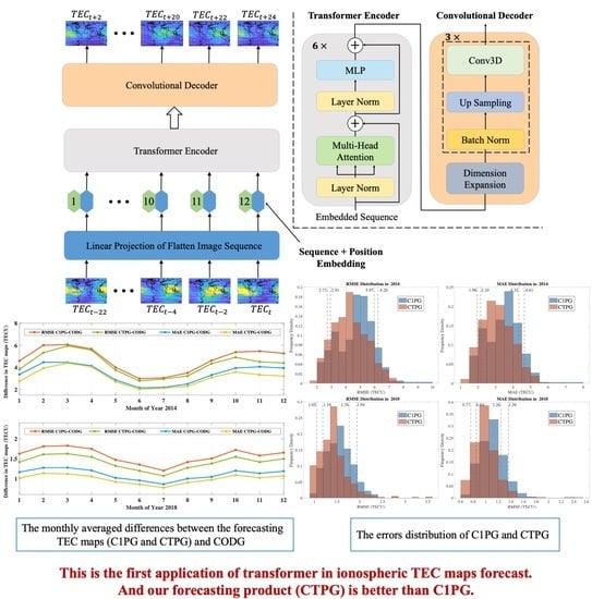
An overview of the model is shown in Figure 1. It can be seen that the CAiTST model adopts the classic sequence-to-sequence and encoder–decoder structure. The CAiTST model first flattens and linearly projects the 12 input TEC maps of the day to obtain image embeddings. Then, the position embeddings are added to obtain a 1D sequence of token embeddings, which is input into the transformer encoder. The transformer encoder mainly consists of layer normalization, multi-head attention mechanism, MLP and residual connections. After the sequence is encoded by the transformer encoder, it is input into the convolutional decoder to restore 12 TEC maps of the next day. It is worth noting that the 12 output TEC maps are independent, and the TEC maps at the end of the sequence do not depend on the TEC map in the first hours. The convolutional decoder mainly consists of dimension expansion, 3D CNN, batch normalization and up sampling. Below we will describe each of these operations in detail.

3.1. Linear Projection of Flatten Images Sequence

The standard transformer receives an input of a 1D sequence of token embeddings. To handle a 3D image sequence, we reshape the image sequence $\mathit{x}\in {\mathbb{R}}^{N\times H\times W\times C}$ into a sequence of flattened 2D images ${\mathit{x}}_f\in {\mathbb{R}}^{N\times (H\times W\times C)}$, where $(H,W)$ is the resolution of the original image, C is the number of channels, and N is the number of images. The transformer uses constant latent vector size D through all of its layers, so we flatten the images and map them to D dimensions with a trainable linear projection (Equation (1)). We refer to the output of this projection as the image embeddings. In this work, for the TEC map sequence, as described in Section 2, $N,H,W,C$ are 12, 71, 73, 1, respectively, and D is set to 324.

$${\mathit{x}}_{emb}={\mathit{x}}_{\mathit{f}}\mathit{E},\mathit{E}\in {\mathbb{R}}^{(H\times W\times C)\times D}$$

(1)

Then, position embeddings [26] are added to the image embeddings to retain positional information, which is given as follows:

$$\begin{array}{c}\mathit{P}{\mathit{E}}_{(pos,2i)}=sin\left(pos/10,{000}^{2i/D}\right)\\ \mathit{P}{\mathit{E}}_{(pos,2i+1)}=cos\left(pos/10,{000}^{2i/D}\right)\end{array}$$

(2)

where $pos$ is the position and i is the dimension. That is, each dimension of the positional encoding corresponds to a sinusoid. Moreover, we can get the input of transformer encoder ${\mathit{z}}_0$.

$${\mathit{z}}_0={\mathit{x}}_{emb}+\mathit{PE}={\mathit{x}}_f\mathit{E}+\mathit{PE},\mathit{PE}\in {\mathbb{R}}^{N\times D}$$

(3)

3.2. Transformer Encoder

The transformer encoder [26] consists of alternating layers of multiheaded self-attention (MSA) and multilayer perceptron (MLP) blocks. Layer normalization (LN) is applied before every block [29], and residual connections after every block [30,31].

3.2.1. Layer Normalization (LN)

We normalize the activities of the neurons is an effective way to address the computationally high cost of training state-of-the-art deep neural networks. LN [29] solves the problem that it is not obvious how to apply batch normalization (BN) to recurrent neural networks (RNNs). BN is converted into LN by calculating the normalized mean and variance from summing all inputs of one layer of neurons in a single training case. By calculating the normalized statistical data at each time step, it can also be directly applied to RNNs. In addition, computing the LN statistics over all the hidden neurons in the same layer is performed as follows:

$${\mu }^l=\frac{1}{H}\sum _{i=1}^H{a}_i^l{\sigma }^l=\sqrt{\frac{1}{H}{\displaystyle \sum _{i=1}^H}{\left(a_i^l-{\mu }^l\right)}^2}$$

(4)

where $a^l$ is the vector representation of the input sum of neurons in this layer and H denotes the number of hidden units in a layer.

3.2.2. Multiheaded Self-Attention (MSA)

In the standard self-attention (SA) mechanism, each element has three different vectors, which are the query vector ($\mathit{Q}$), the key vector ($\mathit{K}$) and the value vector ($\mathit{V}$). They are obtained by multiplying the embedding vector ${\mathit{x}}_{emb}$ by three different weight matrices ${\mathit{W}}_Q$, ${\mathit{W}}_K$ and ${\mathit{W}}_V$, which can be represented by the following formula:

$$[\mathit{Q},\mathit{K},\mathit{V}]=LN\left(\mathbf{z}\right){\mathit{U}}_{qkv},{\mathit{U}}_{qkv}=\left[{\mathit{W}}_Q,{\mathit{W}}_K,{\mathit{W}}_V\right]\in {\mathbb{R}}^{D\times 3D_h}$$

(5)

Then, the attention weights ${\mathit{A}}_j^i$ are based on the scaled inner product computed by the $q^i$ and $k^j$ of the two elements in the sequence.

$$\mathit{A}=softmax\left(\mathit{Q}{\mathit{K}}^T/\sqrt{D}\right),\mathit{A}\in {\mathbb{R}}^{N\times N}$$

(6)

Moreover, we multiply the attention weight matrix $\mathit{A}$ by value vector $\mathit{V}$ to get the output of SA.

$$SA\left(LN\left(\mathit{z}\right)\right)=\mathit{A}\mathit{V}$$

(7)

MSA is an extension of SA in which we run k SA operations in parallel and project their concatenated outputs, and here, k is set to 9. To compute and keep the number of parameters the same when changing k, $D_h$ is typically set to $D/k$, so it is 36 here.

$$MSA(LN\left(\mathit{z}\right))=\left[{SA}_1(LN\left(\mathit{z}\right));{SA}_2(LN\left(\mathit{z}\right));\dots ;{SA}_k(LN\left(\mathit{z}\right))\right]{\mathit{U}}_{msa},{\mathit{U}}_{msa}\in {\mathbb{R}}^{D\times D}$$

(8)

To assist understanding, Figure 2 shows the specific operation of MSA when $N=3$, $D=4$, $D_h=2$ and $k=2$.

3.2.3. Multilayer Perceptron (MLP)

The MLP block consists of a hidden layer and an output layer, the number of neurons in each is 3D and D, respectively, and the activation function is an ELU function. Furthermore, to facilitate the description of input and output of the MLP, in the ℓth module, let the output of the first residual connection be ${\mathit{z}}_{\ell }^{\prime }$, and the output of the second residual connection be ${\mathit{z}}_{\ell }$. Hence we have the following formulas:

$${\mathit{z}}_{\ell }^{\prime }=MSA\left(LN\left({\mathit{z}}_{\ell -1}\right)\right)+{\mathit{z}}_{\ell -1},\ell =1\dots L$$

(9)

$${\mathit{z}}_{\ell }=MLP\left(LN\left({\mathit{z}}_{\ell }^{\prime }\right)\right)+{\mathit{z}}_{\ell }^{\prime },\ell =1\dots L$$

(10)

where L is the number of repetitions of the transformer encoder module. In this work, we employ $L=6$ encoder modules.

3.3. Convolutional Decoder

The convolutional decoder consists of dimension expansion, three CNN blocks and an up sampling layer. In the CNN bocks, batch normalization (BN) [32] is used before every CNN.

3.3.1. Dimension Expansion

The output ${\mathit{z}}_L\in {\mathbb{R}}^{N\times D}$ of the transformer encoder is 2D in keeping with the dimensions of its input. In order to restore the original 3D image sequence, we first expand the output dimension from $N\times D$ to $N\times \sqrt{D}\times \sqrt{D}\times 1$; therefore, D needs to be a square number.

$${\mathit{s}}_0=reshape\left({\mathit{z}}_L\right),{\mathit{s}}_0\in {\mathbb{R}}^{N\times \sqrt{D}\times \sqrt{D}\times 1}$$

(11)

Therefore, in this work, after the dimension expansion, we get the input ${\mathit{s}}_0\in {\mathbb{R}}^{12\times 18\times 18\times 1}$ of the convolutional network block.

3.3.2. Batch Normalization (BN)

BN is proposed to address the internal covariate shift, which slows down the training by requiring lower learning rates and careful parameter initialization [32]. Therefore, in the CNN block, BN is used before every CNN layer, which allows us to use much higher learning rates and be less careful about initialization. For the values of $x$ over a mini-batch ($\mathcal{B}=\left\{x_{1\dots m}\right\}$), BN first calculates it’s mean and variance with the following formulas:

$${\mu }_{\mathcal{B}}=\frac{1}{m}\sum _{i=1}^m{x}_i$$

(12)

$${\sigma }_{\mathcal{B}}^2=\frac{1}{m}\sum _{i=1}^m{\left(x_i-{\mu }_{\mathcal{B}}\right)}^2$$

(13)

The values are then normalized using the obtained mean and variance to obtain values of $\widehat{x}$ that conform to the (0, 1) normal distribution, where $ϵ$ is a tiny positive number used to avoid divisors by 0.

$${\widehat{x}}_i=\frac{x_i-{\mu }_{\mathcal{B}}}{\sqrt{{\sigma }_{\mathcal{B}}^2+ϵ}}$$

(14)

Finally, we multiply $x_i$ by $\gamma$ to adjust the value and add $\beta$ to increase the offset to get $y_i$, where $\gamma$ is the scale factor, and $\beta$ is the translation factor. This step is the essence of BN. Since the normalized $x_i$ will basically be limited to a normal distribution, the expression ability of the network will decrease. Two new parameters $\gamma$ and $\beta$ are introduced to solve this difficulty, which is learned by the network itself during training.

$${BN}_{\gamma ,\beta }\left(x_i\right)=y_i=\gamma {\widehat{x}}_i+\beta$$

(15)

3.3.3. Convolutional Neural Network (CNN)

Since CNN was proposed, it has been widely used in the image field, such as image classification [33], image generation [34], image semantic segmentation [35] and image sequence prediction [36]. The core idea of CNN is that the local area is multiplied by a fixed operation matrix (called convolution kernel filter), and the operation matrix will be reused in different local areas until all pixels participate in the operation. This way of weight sharing and local connectivity will reduce the number of network parameters, making the operation concise and efficient. They also made strong and mostly correct assumptions about the stationarity of image statistical data and the locality of pixel dependence. Therefore, compared with the standard feedforward NN with a similar layer size, CNN has much fewer connections and parameters, so they need less time to converge under the same training conditions, although this will lead to a slightly worse theoretical optimal performance [33].

In this paper, there are three 3D CNNs to decode the TEC maps. The number of convolution kernels of the three convolutional neural networks is 40, 40 and 1, respectively. The sizes of the convolution kernels are all (5, 5, 5), and the activation functions are all the ELU functions. Thus, this progress can be expressed by the following formula:

$${\mathit{s}}_m=\mathrm{Conv} 3\mathrm{D}\left(BN\left({\mathit{s}}_{m-1}\right)\right),m=1\dots M$$

(16)

where M is the number of repetitions of the CNN module. In this paper, $M=3$, and ${\mathit{s}}_1,{\mathit{s}}_2\in {\mathbb{R}}^{12\times 18\times 18\times 40}$ and ${\mathit{s}}_3\in {\mathbb{R}}^{12\times 18\times 18\times 1}$.

3.3.4. Up Sampling

In order to restore the final output size of CNN to the size of the IGS TEC maps, bilinear interpolation is used for up sampling. This step can be expressed as:

$$\mathit{output}=Upsampling\left({\mathit{s}}_3\right),\mathit{output}\in {\mathbb{R}}^{12\times 71\times 73\times 1}$$

(17)

Thus far, we have the 12 TEC maps $\mathit{output}$ with a time resolution of two hours for the next day.

4. Results

As the architecture shown in Figure 1, we used the PyTorch framework to build the CAiTST model, and the hyperparameters of the model are determined by manual tuning. We also used the adaptive moment estimation (ADAM) optimizer with the learning rate set to 0.001. Additionally, the loss function was chosen as the mean square error (MSE) function. Furthermore, a total of 1000 iterations were carried out, and the batch size was set to 32.

4.1. Evaluation Metrics

Here, the root mean square error (RMSE) and mean absolute error (MAE) are used to evaluate the performance of the model. Their formulas are as follows:

$$RMSE=\sqrt{\frac{{\sum }_{j=1}^N{\left(TE{C}_{IGS,j}-TE{C}_{Pre,j}\right)}^2}{N}}$$

(18)

$$MAE=\frac{{\sum }_{j=1}^N\left|TE{C}_{IGS,j}-TE{C}_{Pre,j}\right|}{N}$$

(19)

where, $TE{C}_{IGS,j}$ and $TE{C}_{Pre,j}$ are observations and predictions, respectively, $j=1,2,\dots ,N$, and N represents the total number of data samples.

4.2. Training Set and Validation Set Results Analysis

As we stated in Section 2, we use data from 2005–2013 and 2015–2017 (90% as the training set and 10% as the validation set) to train the model with the architecture shown in Figure 1.

Table 1. Training and validation set loss values (TECU) when $L=3,4,5,6,7,8$.

Repetition Number of the Transformer Encoder Module	Training Loss	Validation Loss
3	8.01	10.69
4	6.24	9.11
5	4.91	8.32
6	4.54	6.01
7	4.38	6.55
8	4.22	6.79

shows the loss values of the training set and the test set after the model is trained for 1000 epochs when $L=3,4,5,6,7,8$. As seen in Table 1, as the number of repetitions L increases, the training loss decreases gradually, which illustrates that more network layers could better fit TEC maps on the previous day and those on the future day. However, starting from $L=7$, as the number of repetitions increases, the validation loss also increases, indicating that the model is overfitting. Therefore, we set $L=6$ in this work. The tuning of other hyperparameters is similar.

After all the hyperparameters are tuned, Figure 3 shows the variation of the training loss and validation loss during the training process. It can be seen that with the increase in training epochs, the training loss and validation loss continue to decrease, and the model successfully converges.

4.3. Test Sets Results Analysis

Data from 2014 (high solar activity year) and 2018 (low solar activity year) are used as the test set. The TEC maps predicted by our CAiTST model and 1-day CODE prediction model are named CTPG and C1PG, respectively. The C1PG has been proven to have better forecasting performance than E1PG and U2PG [37], which are predicted ionospheric products produced by the European Space Operations Center (ESOC) and UPC, respectively. In addition, the superiority of our CAiTST model is assessed by comparing the differences between CTPG and C1PG with respect to CODG. The robustness of the CAiTST model under severe geomagnetic storm disturbance conditions is also investigated.

4.3.1. Comparison of Predicted TEC Maps

Figure 4 shows the monthly averaged RMSE and MAE values between the forecasting TEC maps (C1PG and CTPG) and the IGS TEC maps (CODG) in 2014 and 2018. The RMSEs and MAEs shown in Figure 4 indicate that there is better consistency between CTPG and CODG, especially in January, November, and December of 2014. Additionally, it is worth noting that the performance of the model varies in different seasons. As shown in Figure 4, the RMSE and MAE values in the northern hemisphere’s summer are smaller than those in the northern hemisphere’s spring and winter, both in 2014 and 2018. Moreover,

Table 2. The annual mean RMSE and MAE values (TECU) between forecasting TEC maps (CTPG and C1PG) and IGS TEC maps (CODG) during high and low solar activity periods.

	C1PG		CTPG
	RMSE	MAE	RMSE	MAE
All test data	$3.14$	$2.27$	$2.85$	$2.06$
Solar maximum	$4.71$	$3.44$	$4.29$	$3.12$
Solar minimum	$1.57$	$1.11$	$1.41$	$0.99$

presents the annual mean values of RMSE and MAE values between the predicted TEC maps (CTPG and C1PG) and the IGS TEC maps (CODG) in 2014 and 2018. As shown in Table 2, CTPG performs slightly better than C1PG both in 2014 and 2018. Compared to C1PG in 2014, the annual mean RMSE of the CTPG is approximately 0.4 TECU lower, a decrease of 8.9%, while in 2018, the same value is about 0.2 TECU lower, a decrease of 10.2%. As for MAE, in 2014, the annual mean MAE of CTPG decreased by 9.3% compared to that of C1PG, and in 2018, it decreased by 10.8%. However, the prediction RMSE and MAE values of the same model in 2014 are larger than those in 2018 due to more frequent solar activities and higher background electron density.

Figure 5 below shows the histogram of the error distribution of C1PG and CTPG in 2014 and 2018, with the dotted line marking the 10% position. Taking the RMSE distribution in 2014 as an example, it can be seen that the RMSE of the top 10% and the bottom 10% of CTPG are 2.73 and 5.97 TECU, respectively, which are smaller than the 2.91 and 6.20 TECU of C1PG. Overall, the orange dotted line (CTPG) is always to the left of the blue dotted line (C1PG), which shows that the prediction performance of CTPG is better than that of C1PG.

4.3.2. Latitudinal and Longitudinal Behavior

The latitudinal distribution of CTPG and C1PG prediction performance in 2014 and 2018 is first investigated. The latitudinal behavior of the predicted TEC maps is analyzed by comparing the predicted TEC values with the IGS TEC values at the same latitude. As shown in Figure 6, the changing trends of RMSE and MAE values in the same year are almost the same; it can be seen that the RMSE and MAE curves of CTPG and C1PG in 2018 are very close. However, in 2014, between the two latitude ranges of 87.5°S–${45}^{°}$S and ${30}^{°}$N to ${75}^{°}$N, the RMSE and MAE curves of C1PG are significantly above the RMSE and MAE curves of CTPG. In other words, between these two latitude ranges, the prediction performance of CTPG is significantly better than the performance of C1PG in 2014. Further, note in the low latitude region (${30}^{°}$S–${30}^{°}$N), the RMSE and MAE curves of the CTPG and C1PG show a double-peak structure, which is similar to the structure of TEC values in the equatorial ionospheric anomaly (EIA) region; this structure is more obvious in the high solar activity year than in the low solar activity year. Hence, TEC values in the EIA area are more difficult to predict accurately than those in other areas. The RMSE values in 2018 are within 1–2 TECU, much lower than the 3–7 TECU in 2014.

Table 3. RMSE and MAE values between the predicted TEC maps (CTPG and C1PG) and IGS TEC maps (CODG) in different latitude regions in 2014 and 2018.

	2014			2018
	High Latitudes	Middle Latitudes	Low Latitudes	High Latitudes	Middle Latitudes	Low Latitudes
$\mathbf{RMSE}\left(\mathbf{TECU}\right)$
CTPG	$3.41$	$3.63$	$5.81$	$0.92$	$1.20$	$1.95$
C1PG	$4.09$	$4.29$	$5.92$	$1.12$	$1.37$	$2.12$
$\mathbf{MAE}\left(\mathbf{TECU}\right)$
CTPG	$2.52$	$2.64$	$4.18$	$0.71$	$0.88$	$1.38$
C1PG	$2.95$	$3.12$	$4.23$	$0.82$	$1.00$	$1.50$

demonstrates the mean RMSE and MAE values of CTPG and C1PG in high latitude (87.5°S(N)–${60}^{°}$S(N)), middle latitude (57.5°S(N)–${30}^{°}$S(N)) and low latitude (27.5°S–27.5°N) regions in 2014 and 2018. It can be seen that the RMSE and MAE values of CTPG are smaller than those of C1PG in all three regions, and the difference is more pronounced in the high and middle latitude regions. Taking the RMSE values in 2014 as an example, the RMSE of CTPG decreased by 16.6% and 15.4% in the high and middle latitude regions, respectively, compared with the RMSE of C1PG, but only decreased by 1.8% in the low latitude region. This illustrates that CAiTST performs better at middle and high latitudes than at low latitudes.

In addition, we also investigate the geographic distribution of the performance of predicted TEC maps at the level of a grid point. Figure 7 and Figure 8 demonstrate the maps showing the RMSE and MAE of CTPG and C1PG with respect to CODG in 2014 and 2018. As shown in Figure 7, in 2014, the largest RMSE value is about 9 TECU in the EIA region, while in 2018, it is less than 3 TECU. This result may be explained by the more frequent solar activity in 2014. In addition, the RMSE and MAE values in the EIA area are higher than those in other areas, particularly in 2014. However, the CTPG evidently outperforms C1PG in the EIA region. Furthermore, due to the sparse distribution of GNSS stations in the marine area, the accuracy of the marine area is usually lower than that of the continental area on the GIMs [38]. It may explain that the RMSE and MAE values between C1PG and CODG in the continental area are obviously smaller than those in the ocean area. The performance of CTPG in the marine area is obviously better than that of C1PG. In summary, Figure 7 and Figure 8 present that CTPG has better consistency with the CODG than C1PG.

In order to visually observe the differences between CTPG and CODG, the TEC maps of CTPG and CODG at 00:00, 06:00, 12:00 and 18:00 UT on the spring equinox, summer solstice, autumn equinox and winter solstice in 2014 and 2018 are shown in Figure 9 and Figure 10. In each panel of these two figures, the maps in the first and second rows are CODE TEC maps and CTPG TEC maps, respectively, and the maps in the third row are the difference maps between CODG and CTPG TEC maps, which are defined as:

$$DTEC=TE{C}_{Pre}-TE{C}_{\mathrm{IGS}}$$

(20)

where $TE{C}_{Pre}$ is the predicted global TEC maps (CTPG), and $TE{C}_{\mathrm{IGS}}$ is the IGS global TEC maps (CODE).

In panel a of Figure 9, at 00:00 UT, although CAiTST predicts the location of EIA well, the TEC values in the EIA region are obviously underestimated, and this underestimation is mitigated in the following predicted TEC maps. It can be seen from these two figures that although CTPG has the largest error in the EIA area, it still predicts the characteristics and location of the EIA well, and the predicted EIA region has a good similarity with the CODG. It is worth noting that in panel d of Figure 9, it can be seen from the DTEC maps that the performance of CTPG decreased because a magnetic storm occurred on 22 December 2014. This is exactly what will be discussed in detail in the next subsection. Since the CAiTST only contains the past TEC maps as the input and the information related to magnetic storms cannot be obtained only from the past TEC maps, the performance of the CTPG will decline during magnetic storms.

4.3.3. Performance for Different TEC Maps Sources

To evaluate the performance of the CAiTST for different TEC maps sources, the TEC maps released by six other IAACs (Chinese Academy of Sciences (CAS), European Space Agency (ESA), IGS, Jet Propulsion Laboratory (JPL), UPC and Wuhan University (WHU)) are forecasted by CAiTST in 2014 and 2018.

Table 4. RMSE and MAE values between the predicted TEC maps (using the TEC maps of the corresponding source as input) and the different TEC maps released by different IAACs in 2014 and 2018.

GIMs ID	RMSE			MAE
	Solar Maximum	Solar Minimum	Overall	Solar Maximum	Solar Minimum	Overall
CASG	4.27	1.45	2.86	3.12	1.02	2.07
CODG	4.29	1.41	2.85	3.12	0.99	2.06
ESAG	4.65	1.58	3.12	3.47	1.16	2.32
IGSG	4.10	1.56	2.83	3.03	1.13	2.08
JPLG	4.58	2.06	3.32	3.47	1.58	2.53
UPCG	4.54	1.68	3.11	3.45	1.21	2.33
WHUG	4.61	1.73	3.17	3.37	1.24	2.31

shows the RMSE and MAE values between the predicted TEC maps (using the TEC maps of the corresponding source as input) and the different TEC maps. As shown in Table 4, CASG, ESAG, JPLG, UPCG, WHUG and IGSG represent the final TEC maps provided by CAS, ESA, JPL, UPC, WHU and IGS, respectively. As seen in Table 4, in 2014, the performance of the model for the IGSG is the best, with an RMSE and MAE of 4.10 and 3.03 TECU, respectively, which are both smaller than 4.29 and 3.12 TECU for CODG. Additionally, the performance of the model for CASG is also slightly better than that for CODG, although the training of the model is implemented on the CODG. However, in 2018, the performance for CODG TEC maps is the best, and that for JPLG is the worst, with an RMSE exceeding 2 TECU.

4.3.4. Performance during Magnetic Storm

It is difficult for the ionospheric prediction model to work effectively for geomagnetic storm days [39]. To evaluate the performance of CTPG during a geomagnetic storm period, we analyze the differences between the predicted TEC maps and CODG during the magnetic storm period ($\mathrm{Dst}<-30\mathrm{nT}$ [40,41]) and calm period, which are shown in

Table 5. RMSE and MAE values between the predicted TEC maps (CTPG and C1PG) and the IGS TEC maps (CODG) during a magnetic storm and a calm period in 2014 and 2018.

Period	Dst	Metric	2014		2018
			CTPG	C1PG	CTPG	C1PG
Storm	<$-30\mathrm{nT}$	RMSE	$5.38$	$6.02$	$2.09$	$2.20$
		MAE	$4.01$	$4.52$	$1.36$	$1.55$
Calm	>$-30\mathrm{nT}$	RMSE	$4.12$	$4.48$	$1.47$	$1.52$
		MAE	$3.01$	$3.31$	$0.97$	$1.09$

. It can be seen from the table that when a magnetic storm occurs, the forecasting performance of CTPG decreases significantly, which is the same as that of C1PG. However, in both 2014 and 2018, CTPG still outperforms C1PG, with or without a magnetic storm.

Given two intense magnetic storm events that occurred on 28 February 2014 and 26 August 2018. Similar to Figure 9 and Figure 10, Figure 11 shows the comparison between the CODG and CTPG for these two days. As shown in Figure 11, when the magnetic storm occurs on 28 February 2014, the prediction error of the model in the EIA region is the largest, and the CAiTST under-predicts in most of the EIA region. Moreover, the prediction error of the model in the southern hemisphere is larger than that in the northern hemisphere, and there is an over-prediction. In Figure 9, the model still under-predicts in the EIA area at 00:00, 06:00, and 12:00 on 26 August 2018, but over-predicts at 18:00. The above results shows that CAiTST fails to capture such complex and rapid changes in the EIA region during magnetic storms with only past TEC maps as input.

5. Discussion

In this paper, forecasting the TEC maps is regarded as an image time sequence prediction problem. Each TEC map contains not only the TEC value of each grid point but also rich spatial information (longitude and latitude information). The chronological sequence of TEC maps also contains temporal information. Therefore, a forecasting model of the TEC map sequence needs to have the ability to process both spatial and temporal features. As transformer has incomparable advantages in time series prediction because of its unique self-attention mechanism, we develop a transformer-based TEC map sequence prediction model named CAiTST. By dividing an image into a certain number of subgraphs and then performing linear projection on them, transformer can also replace the traditional convolution operation to process the image. Inspired by this, the 2D TEC map is linearly projected into the 1D embedding so that the transformer can be used as an encoder to encode a 12 TEC map sequence in a day, and then the 3D CNN is added as a decoder. To accelerate the training speed of the CAiTST, LN and BN are used in the encoder and decoder, respectively. The training, verification and testing of the model are all completed by the CODE final TEC map products (CODG). The data from 2005 to 2018 constitute the training set (90% of total) and verification set (10% of total), and the test set consists of the data from the high solar activity year (2014) and low solar activity year (2018). In the test stage, RMSE and MAE are selected as evaluation metrics to investigate the performance of the model. Compared with the results of the CODE one-day prediction product (C1PG), the superiority of the CAiTST model is verified.

The results show that CTPG (TEC map products predicted by CAiTST) performs better than C1PG in both 2014 and 2018. The RMSE values of CTPG with respect to CODG decreased by 8.9% and 10.2% compared with those of C1PG in 2014 and 2018, respectively, while the MAE values decreased by 9.3% and 10.8%. The results also illustrate that the prediction performance depends on the season. The two predicted products both perform better in summer than in spring and winter. In addition, by the analysis of latitudinal behavior, it can be concluded that the errors of the two predicted products in the low latitudes are greater than those in the high and middle latitudes due to anomalies in the low latitudes such as EIA and the high background electron density. Furthermore, through the analysis of the geographic distribution of the performance, the results show that the EIA region is the most difficult to predict. It may be explained by the inaccuracy of the IGS TEC maps representing well-known ionospheric structures such as the EIA [10]. Because GNSS stations are sparsely distributed in marine areas, C1PG has obvious errors in marine areas, where CTPG is not significantly impacted. This shows that our model is not affected by the lower accuracy of the IGS TEC maps in the southern hemisphere than in the northern hemisphere [42].

It is worth noting that in most of the TEC prediction research, the past TEC values, which are highly correlated with the future TEC values [43], are often used as the input of the forecasting model.

Table 6. Annual mean RMSE and MAE values (TECU) between 12 TEC maps for the past day and 12 TEC maps for the future day during high and low solar activity periods.

	RMSE	MAE
All test data	3.23	2.26
Solar maximum	4.84	3.45
Solar minimum	1.61	1.07

shows the annual mean RMSE and MAE values between 12 TEC maps in the past day and 12 TEC maps in the future day during high and low solar activity periods. The reason why we compare the copy of 12 TEC maps from the past day rather than the average of TEC maps from the past two or three days is because that is the input for our model. According to Table 2 and Table 6, in 2014, the RMSE values between the predicted TEC maps (C1PG and CTPG) and CODG are 1.57 and 1.41 TECU, and the RMSE between CODG maps of the previous day and CODG maps of the future day is 1.61 TECU. In addition, it can be seen that in the whole test dataset, the RMSE values between predicted TEC maps and future TEC maps decrease by 11.8% compared to those between past TEC maps and future TEC maps, and the MAE values decrease by 8.9%. This illustrates that our CAiTST model has indeed learned the relationship between the past TEC maps and future TEC maps and successfully made predictions. Furthermore, in order to prove the effectiveness of the prediction model, we suggest that in future TEC prediction work, if the prediction model uses the past TEC value as input, the copy or average of the past TEC values should also be included in the evaluation.

We also evaluate the performance of CAiTST for different TEC map sources. Although the CAiTST model is trained by CODG, in 2014, the performance for IGSG is the best, and the performance for ESAG is the worst. In 2018, the model performs best for CODG and performs worst for JPLG. The results illustrate that our model could be applied to the prediction of different TEC maps sources.

The performance of CAiTST during a magnetic storm is also investigated. However, the results suggest that when a storm occurs, CAiTST fails to capture the complex and rapid changes of TEC, especially in the EIA region. This is mainly because our model only includes past TEC maps as the input, no information relating to a prior storm is considered in the model. When the TEC maps are used as the input for the neural network, it is hard to add other additional parameters as input at the same time, which prevents us from adding other parameters, such as Dst or Kp index, to represent the information relating to prior storms.

Therefore, in future work, how to use the TEC maps and some individual parameters, including storm information, as inputs to the transformer model at the same time is the next focus to be studied. Only then does the model have the possibility to work properly during a storm period. Moreover, the performance degradation of the model in the EIA region also needs further research to be solved, and developing a regional prediction model can alleviate it. Other deep learning models, such as GRU [36] and deep generative models [44], may address these above challenges, which will be our follow-up work.

6. Conclusions

In this work, we solve the problem that the traditional transformer model can only be applied to the prediction of the 1D matrix sequence. The proposed transformer model is successfully used to predict the 2D global TEC maps sequence, which is a whole new potential model in the ionosphere model research community utilizing deep learning techniques. The results show that our CAiTST model has good accuracy in both high and low solar activity years, and its performance is better than the 1-day CODE prediction model. These results also demonstrate that the transformer model models the relationship between past TEC values and future TEC values well. In general, our model is competitive in short-term global TEC map forecasting, and it is instructive for the study of transformer models in space and weather. Furthermore, our model can also provide new ideas for other fields of image sequence prediction, such as precipitation nowcasting using radar.

References

- Lastovicka, J.; Urbar, J.; Kozubek, M. Long-term trends in the total electron content. Geophys. Res. Lett. 2017, 44, 8168–8172. [Google Scholar] [CrossRef]
- Ratnam, D.V.; Vishnu, T.R.; Harsha, P.B. Ionospheric gradients estimation and analysis of S-band navigation signals for NAVIC system. IEEE Access 2018, 6, 66954–66962. [Google Scholar] [CrossRef]
- Prol, F.D.; Camargo, P.D.; Monico, J.F.; Muella, M.T. Assessment of a TEC calibration procedure by single-frequency PPP. GPS Solut. 2018, 22, 35. [Google Scholar] [CrossRef]
- Li, Z.; Wang, N.; Wang, L.; Liu, A.; Yuan, H.; Zhang, K. Regional ionospheric TEC modeling based on a two-layer spherical harmonic approximation for real-time single-frequency PPP. J. Geod. 2019, 93, 1659–1671. [Google Scholar] [CrossRef]
- Poniatowski, M.; Nykiel, G. Degradation of kinematic PPP of GNSS stations in central Europe caused by medium-scale traveling ionospheric disturbances during the st. patrick’s day 2015 geomagnetic storm. Remote Sens. 2020, 12, 3582. [Google Scholar] [CrossRef]
- Béniguel, Y. Global Ionospheric Propagation Model (GIM): A propagation model for scintillations of transmitted signals. Radio Sci. 2002, 37, 1–14. [Google Scholar] [CrossRef]
- Qi, F.; Lv, H.; Wang, J.; Fathy, A.E. Quantitative evaluation of channel micro-Doppler capacity for MIMO UWB radar human activity signals based on time–frequency signatures. IEEE Trans. Geosci. Remote Sens. 2020, 58, 6138–6151. [Google Scholar] [CrossRef]
- Feng, J.; Han, B.; Zhao, Z.; Wang, Z. A new global total electron content empirical model. Remote Sens. 2019, 11, 706. [Google Scholar] [CrossRef]
- Feltens, J.; Schaer, S. IGS Products for the Ionosphere. In Proceedings of the 1998 IGS Analysis Center Workshop Darmstadt, Darmstadt, Germany, 9 February 1998; pp. 3–5. [Google Scholar]
- Jee, G.; Lee, H.B.; Kim, Y.H.; Chung, J.K.; Cho, J. Assessment of GPS global ionosphere maps (GIM) by comparison between CODE GIM and TOPEX/Jason TEC data: Ionospheric perspective. J. Geophys. Res. Space Phys. 2010, 115, A10. [Google Scholar] [CrossRef]
- Tang, J.; Yao, Y.; Zhang, L. Temporal and spatial ionospheric variations of 20 April 2013 earthquake in Yaan, China. IEEE Geosci. Remote Sens. Lett. 2015, 12, 2242–2246. [Google Scholar] [CrossRef]
- Lissa, D.; Srinivasu, V.K.; Prasad, D.S.; Niranjan, K. Ionospheric response to the 26 August 2018 geomagnetic storm using GPS-TEC observations along 80 E and 120 E longitudes in the Asian sector. Adv. Space Res. 2020, 66, 1427–1440. [Google Scholar] [CrossRef]
- Hernández-Pajares, M.; Juan, J.M.; Sanz, J.; Orus, R.; Garcia-Rigo, A.; Feltens, J.; Komjathy, A.; Schaer, S.C.; Krankowski, A. The IGS VTEC maps: A reliable source of ionospheric information since 1998. J. Geod. 2009, 83, 263–275. [Google Scholar] [CrossRef]
- Shi, C.; Gu, S.; Lou, Y.; Ge, M. An improved approach to model ionospheric delays for single-frequency precise point positioning. Adv. Space Res. 2012, 49, 1698–1708. [Google Scholar] [CrossRef]
- Rovira-Garcia, A.; Juan, J.M.; Sanz, J.; González-Casado, G. A worldwide ionospheric model for fast precise point positioning. IEEE Trans. Geosci. Remote Sens. 2015, 53, 4596–4604. [Google Scholar] [CrossRef]
- Schaer, S. Mapping and Predicting the Earth’s Ionosphere Using the Global Positioning System. Ph.D. Thesis, University Bern, Bern, Switzerland, 1999. [Google Scholar]
- García-Rigo, A.; Monte, E.; Hernández-Pajares, M.; Juan, J.M.; Sanz, J.; Aragón-Angel, A.; Salazar, D. Global prediction of the vertical total electron content of the ionosphere based on GPS data. Radio Sci. 2011, 46, 1–3. [Google Scholar] [CrossRef]
- Jakowski, N.; Mayer, C.; Hoque, M.M.; Wilken, V. Total electron content models and their use in ionosphere monitoring. Radio Sci. 2011, 46, 1–11. [Google Scholar] [CrossRef]
- Wang, C.; Xin, S.; Liu, X.; Shi, C.; Fan, L. Prediction of global ionospheric VTEC maps using an adaptive autoregressive model. Earth Planets Space 2018, 70, 18. [Google Scholar] [CrossRef]
- Liu, L.; Zou, S.; Yao, Y.; Wang, Z. Forecasting global ionospheric TEC using deep learning approach. Space Weather 2020, 18, e2020SW002501. [Google Scholar] [CrossRef]
- Tang, J.; Li, Y.; Yang, D.; Ding, M. An Approach for Predicting Global Ionospheric TEC Using Machine Learning. Remote Sens. 2022, 14, 1585. [Google Scholar] [CrossRef]
- Lee, S.; Ji, E.Y.; Moon, Y.J.; Park, E. One-Day Forecasting of Global TEC Using a Novel Deep Learning Model. Space Weather 2021, 19, 2020SW002600. [Google Scholar] [CrossRef]
- Lin, X.; Wang, H.; Zhang, Q.; Yao, C.; Chen, C.; Cheng, L.; Li, Z. A Spatiotemporal Network Model for Global Ionospheric TEC Forecasting. Remote Sens. 2022, 14, 1717. [Google Scholar] [CrossRef]
- Chen, Z.; Liao, W.; Li, H.; Wang, J.; Deng, X.; Hong, S. Prediction of global ionospheric TEC based on deep learning. Space Weather 2022, 20, e2021SW002854. [Google Scholar] [CrossRef]
- Xia, G.; Zhang, F.; Wang, C.; Zhou, C. ED-ConvLSTM: A Novel Global Ionospheric Total Electron Content Medium-term Forecast Model. Space Weather 2022, 20, e2021SW002959. [Google Scholar] [CrossRef]
- Vaswani, A.; Shazeer, N.; Parmar, N.; Uszkoreit, J.; Jones, L.; Gomez, A.N.; Kaiser, Ł; Polosukhin, I. Attention is all you need. In Proceedings of the Advances in Neural Information Processing Systems 30: Annual Conference on Neural Information Processing Systems, Long Beach, CA, USA, 4–9 December 2017; pp. 5998–6008. [Google Scholar]
- Dosovitskiy, A.; Beyer, L.; Kolesnikov, A.; Weissenborn, D.; Zhai, X.; Unterthiner, T.; Dehghani, M.; Minderer, M.; Heigold, G.; Gelly, S.; et al. An image is worth 16 × 16 words: Transformers for image recognition at scale. arXiv 2020, arXiv:2010.11929. [Google Scholar]
- Jee, G.; Schunk, R.W.; Scherliess, L. Analysis of TEC data from the TOPEX/Poseidon mission. J. Geophys. Res. Space Phys. 2004, 109, A01301. [Google Scholar] [CrossRef]
- Ba, J.L.; Kiros, J.R.; Hinton, G.E. Layer normalization. arXiv 2016, arXiv:1607.06450. [Google Scholar]
- Wang, H.; Zhu, Y.; Green, B.; Adam, H.; Yuille, A.; Chen, L.C. Axial-deeplab: Stand-alone axial-attention for panoptic segmentation. In Computer Vision—ECCV 2020, Proceedings of the 16th European Conference, Glasgow, UK, 23–28 August 2020; Springer International Publishing: Cham, Switzerland, 2020; pp. 108–126. [Google Scholar]
- Baevski, A.; Auli, M. Adaptive Input Representations for Neural Language Modeling. arXiv 2018, arXiv:1809.10853. [Google Scholar]
- Ioffe, S.; Normalization, C.S. Batch Normalization: Accelerating deep network training by reducing internal covariate shift. arXiv 2014, arXiv:1502.03167. [Google Scholar]
- Krizhevsky, A.; Sutskever, I.; Hinton, G.E. Imagenet classification with deep convolutional neural networks. In Proceedings of the Twenty-Sixth Annual Conference on Neural Information Processing Systems (NIPS), Lake Tahoe, NV, USA, 3–8 December 2012; p. 25. [Google Scholar]
- Zhang, J.; Chen, L.; Zhuo, L.; Liang, X.; Li, J. An efficient hyperspectral image retrieval method: Deep spectral-spatial feature extraction with DCGAN and dimensionality reduction using t-SNE-based NM hashing. Remote Sens. 2018, 10, 271. [Google Scholar] [CrossRef]
- Zhang, C.; Zhou, J.; Wang, H.; Tan, T.; Cui, M.; Huang, Z.; Wang, P.; Zhang, L. Multi-Species Individual Tree Segmentation and Identification Based on Improved Mask R-CNN and UAV Imagery in Mixed Forests. Remote Sens. 2022, 14, 874. [Google Scholar] [CrossRef]
- Ruwali, A.; Kumar, A.S.; Prakash, K.B.; Sivavaraprasad, G.; Ratnam, D.V. Implementation of hybrid deep learning model (LSTM-CNN) for ionospheric TEC forecasting using GPS data. IEEE Geosci. Remote Sens. Lett. 2020, 18, 1004–1008. [Google Scholar] [CrossRef]
- Li, M.; Yuan, Y.; Wang, N.; Li, Z.; Huo, X. Performance of various predicted GNSS global ionospheric maps relative to GPS and JASON TEC data. GPS Solut. 2018, 22, 55. [Google Scholar] [CrossRef]
- Li, W.; Huang, L.; Zhang, S.; Chai, Y. Assessing global ionosphere TEC maps with satellite altimetry and ionospheric radio occultation observations. Sensors 2019, 19, 5489. [Google Scholar] [CrossRef] [PubMed]
- Kim, J.H.; Kwak, Y.S.; Kim, Y.; Moon, S.I.; Jeong, S.H.; Yun, J. Potential of Regional Ionosphere Prediction Using a Long Short-Term Memory Deep-Learning Algorithm Specialized for Geomagnetic Storm Period. Space Weather 2021, 19, e2021SW002741. [Google Scholar] [CrossRef]
- Gonzalez, W.D.; Joselyn, J.A.; Kamide, Y.; Kroehl, H.W.; Rostoker, G.; Tsurutani, B.T.; Vasyliunas, V.M. What is a geomagnetic storm? J. Geophys. Res. Space Phys. 1994, 99, 5771–5792. [Google Scholar] [CrossRef]
- Mukhtarov, P.; Andonov, B.; Pancheva, D. Global empirical model of TEC response to geomagnetic activity. J. Geophys. Res. Space Phys. 2013, 118, 6666–6685. [Google Scholar] [CrossRef]
- Feng, J.; Zhang, T.; Han, B.; Zhao, Z. Analysis of spatiotemporal characteristics of internal coincidence accuracy in global TEC grid data. Adv. Space Res. 2021, 68, 3365–3380. [Google Scholar] [CrossRef]
- Xia, G.; Liu, Y.; Wei, T.; Wang, Z.; Huang, W.; Du, Z.; Zhang, Z.; Wang, X.; Zhou, C. Ionospheric TEC forecast model based on support vector machine with GPU acceleration in the China region. Adv. Space Res. 2021, 68, 1377–1389. [Google Scholar] [CrossRef]
- Ravuri, S.; Lenc, K.; Willson, M.; Kangin, D.; Lam, R.; Mirowski, P.; Fitzsimons, M.; Athanassiadou, M.; Kashem, S.; Madge, S.; et al. Skilful precipitation nowcasting using deep generative models of radar. Nature 2021, 597, 672–677. [Google Scholar] [CrossRef]
Figure 1.
Model overview. We flatten the TEC maps into 1D matrices, linearly embed each of them, add position embeddings and feed the embedding image sequence of vectors to a standard transformer encoder. Then, a decoder consisting of convolutional neural networks and an up sampling layer is responsible for outputting the prediction results.
Figure 2.
The specific operation of the MSA, taking , , and as an example.
Figure 3.
Variation curve of training set loss and validation set loss error with epoch.
Figure 4.
The monthly averaged differences between the forecasting TEC maps (C1PG and CTPG) and IGS TEC maps (CODG) during high and low solar activity periods.
Figure 5.
The errors distribution of C1PG and CTPG in 2014 and 2018.
Figure 6.
RMSE and MAE values between forecasting TEC maps (CTPG and C1PG) and IGS TEC maps (CODG) at different latitudes in 2014 and 2018.
Figure 7.
RMSE values between predicted TEC maps (CTPG and C1PG) and the IGS TEC maps (CODG) in 2014 and 2018. (a) RMSE of CTPG in 2014. (b) RMSE of C1PG in 2014. (c) RMSE of CTPG in 2018. (d) RMSE of C1PG in 2018.
Figure 8.
MAE values between predicted TEC maps (CTPG and C1PG) and the IGS TEC maps (CODG) in 2014 and 2018. (a) MAE of CTPG in 2014. (b) MAE of C1PG in 2014. (c) MAE of CTPG in 2018. (d) MAE of C1PG in 2018.
Figure 9.
Comparison between the CTPG TEC maps and the CODE TEC maps at 00:00, 06:00, 12:00 and 18:00 UT on (a) 21 March 2014, (b) 20 June 2014, (c) 23 September 2014 and (d) 22 December 2014.
Figure 10.
Comparison between the CTPG TEC maps and the CODE TEC maps at 00:00, 06:00, 12:00 and 18:00 UT on (a) 21 March 2018, (b) 20 June 2018, (c) 23 September 2018 and (d) 22 December 2018.
Figure 11.
Comparison between the CTPG TEC maps and the CODE TEC maps at 00:00, 06:00, 12:00 and 18:00 UT on (a) 28 February 2014 and (b) 26 August 2018.