Identification of the Spring Green-Up Date Derived from Satellite-Based Vegetation Index over a Heterogeneous Ecoregion

Abstract

Multiple methods have been developed to identify the transition threshold from the reconstructed satellite-derived normalized difference vegetation indices (NDVI) time series and to determine the inflection point corresponding to a certain phenology phase (e.g., the spring green-up date (GUD)). We address an issue that large uncertainties might occur in the inflection point identification of spring GUD using the traditional satellite-based methods since different vegetation types exhibit asynchronous phenological phases over a heterogeneous ecoregion. We tentatively developed a Maximum-derivative-based (MDB) method and provided inter-comparisons with two traditional methods to detect the turning points by the reconstructed time-series data of NDVI for identifying the GUD against long-term observations from the sites covered by a mixture of deciduous forest and herbages in the Pan European Phenology network. Results showed that higher annual mean temperature would advance the spring GUD, but the sensitive magnitudes differed depending on the vegetation type. Therefore, the asynchronization of phenological phases among different vegetation types would be more pronounced in the context of global warming. We found that the MDB method outperforms two other traditional methods (the 0.5-threshold-based method and the maximum-ratio-based method) in predicting the GUD of the subsequent-green-up vegetation type when compared with ground observation, especially at sites with observed GUD of herbages earlier than deciduous forest, while the Maximum-ratio-based method showed better performance for identifying GUDs of the foremost-green-up vegetation type. Although the new method improved in our study is not universally applicable on a global scale, our results, however, highlight the limitation of current inflection point identify algorithms in predicting the GUD derived from satellite-based vegetation indices datasets in an ecoregion with heterogeneous vegetation types and asynchronous phenological phases, which makes it helpful for us to better predict plant phenology on an ecoregion-scale under future ongoing climate warming.

1. Introduction

As the stages of periodic phenomena in the plant life cycle, vegetation phenology is one of the critical ecological indicators of climate change and has inevitable feedback effects on the climate system by altering the water, energy, and carbon exchange between the terrestrial ecosystem and the atmosphere [1,2,3,4,5,6]. Numerous studies indicate that climate change has resulted in shifts in plant phenology over regional or global scales [6,7,8,9], like the widely reported earlier vegetation green-up onset in spring [9,10,11], which could alter the length and strength of the vegetation growing season and further impact the carbon cycle [7,12,13]. Therefore, increasing efforts have been paid to improve the accuracy of spring vegetation phenological observation and estimation at a larger scale, and the results are helpful for us to understand the impacts of climate change on plant phenology and even the material cycle and energy flow in terrestrial ecosystems, and in turn feedback on climate change [7,14,15].

The majority of previous phenology studies relied on in situ observations of interannual variation in phenological events at the species level. However, such approaches must be limited by the quantity of ground observation sites, and thus, it is nearly impossible to obtain effective information about the interannual variations of plant phenology responses to climate change on a larger scale [16,17]. For the past few years, due to the high consistency between satellite-based indicators and the in situ observed phenological features, remote-sensing techniques have been widely applied in large-scale and long-term plant dynamics observations [6,18,19,20], providing a convenient method to observe vegetation phenology [21,22,23]. Multiple methods have been proposed to identify the key spring vegetation phenological phases (e.g., green-up date, GUD) by estimating inflection points derived from the satellite-based vegetation indices time series datasets (e.g., normalized difference vegetation indices (NDVI)) [24,25,26]. Two main processes are involved in these methods for determining the spring vegetation GUD. The first process is to fit various logistic regression models with the corresponding satellite-derived vegetation indices dataset and obtain higher-temporal-resolution time series datasets that are suitable for vegetation phenological study [27,28]. The second process is to determine the critical turning point for the vegetation GUD from the reconstructed time-series datasets of vegetation indices based on certain rules [6,29]. Generally, there are also two types of rules that have been developed to determine the turning point based on the seasonal variation of vegetation indices. The first one is threshold-based and uses the relative threshold [30] or absolute threshold [31] of vegetation indices to identify the GUD during the growing season [32,33]. Another is ratio-based and identifies the onset of GUD in spring as the date when the increase rate of vegetation indices reaches its maximum value [18,21,29].

However, lots of studies have found that the spring green-up date of deciduous forests estimated by satellite-derived vegetation indices have systematic errors and lack of accuracy [29,34]. Previous research has highlighted the significant differences between identified vegetation GUDs from satellite observations and ground observations [15,35]. For example, researchers compared satellite-derived results against long-term field-based observations and found an absolute difference of up to 26 days for the GUDs of a deciduous broadleaf forest [36]. Wu et al. (2017) [19] compared different satellite-based methods for estimating the growing season onset, and all of them showed relatively low correlation with the observed results of eddy flux measured at 60 sites. Many reasons will lead to the deviation of prediction results [27,37], but the main issue, i.e., the scale-up vs. mixed-pixel problem, is hard to shift, but perhaps unavoidable [26,38]. Although the spatial resolution of satellite-derived vegetation index products has been improved in recent years, a given pixel may include a combination of different vegetation types that might result in significantly different phenology, which challenges the determination of a reliable onset date of spring phenological phases within a heterogeneous ecoregion. Several studies have found significant differences in phenological phase between some deciduous forest and understory or adjacent herbaceous species [29,39,40], which confounds remote sensing metrics and affects the identification of deciduous forest GUD. In addition, many herbaceous species have been shown to emerge earlier than temperate deciduous forest in the spring season in order to take advantage of a short-term growth environment with sufficient light [41,42]. The GUD obtained from the Pan European Phenology (PEP) Database (PEP725; http://www.pep725.eu/ (accessed on 15 July 2021)) revealed a clear distinction between deciduous forest and herbage (Figure 1a,b). Therefore, such a heterogeneous site is difficult to describe with a conventional vegetation index threshold. That is, a large increase in NDVI might occur when the onset date of herbaceous species green up is earlier than that of deciduous forest in the same ecoregion [34]. For such complex scenes, the critical turning point diagnostic rule should be more flexible when using time series of satellite-derived vegetation indexes to extract spring phenological transition in an ecoregion mixed with deciduous forest and herbages.

In this study, we hypothesized that estimating the GUD based on the satellite-derived vegetation index time-series data, especially in an ecoregion mainly covered with deciduous forests and herbages, would suffer from large uncertainties in turning point determination due to the asynchronous onset date of spring phenological phase in different vegetation types. Our study developed the threshold-based determination method, which we refer to as Maximum-derivative-based method (hereafter referred to as the MDB method), to improve estimates of turning points from satellite-derived NDVI time-series data, which is mainly affected by the greenness signal of different vegetation with asynchronous phenological phases. Different from the traditional method that uses the NDVI value mixed with different vegetation types to represent the deciduous forest greenness in a target pixel, the new method further considers the issue that asynchronization of phenological onset date for different vegetation types might affect the turning point identification based on NDVI time-series datasets. As an effort to improve the accuracy of identifying the onset date of vegetation green up in spring, we first fit the annual NDVI time-series datasets with a six-degree polynomial function, which was first used for phenological identification by Piao et al. (2006) and has been proven applicable to the regression in most cases [9,16]. Then we provide inter-comparisons between the improved method and two traditional methods (0.5-threshold-based method and Maximum-ratio-based method) to detect the turning points in the reconstructed time-series data of NDVI for identifying the GUD against long-term observations from the sites of the PEP network, which covered a mixture of deciduous forest and herbages.

2. Materials and Methods

2.1. Ground-Based Observation of GUDs

We obtain the ground-based observations of GUDs from the PEP Database, which provides an open European phenological database comprising 9 million records for 78 species over approximately 20,000 locations across Europe, mainly in Germany, starting in the year 1868. According to the vegetation species, we have filtered out the deciduous forests and herbaceous species and associated them based on the PEP ID. In this study, we selected sites mainly composed of deciduous forests and herbages, and these sites were referred to as forest-herbage-mixed (FHM) sites. We assumed that these two jointly influence the time series of NDVI, a proxy of total vegetation greenness, in a target pixel. We also excluded the FHM sites if the vegetation GUD was later than 180 days of the year and focused on the sites with >25 years of records from 1982 to 2013 to eliminate the potential deviations caused by abnormal values. To focus on the most reliable pair of ground observations and satellite observations, only those grid zones covering vegetation types (deciduous forests and herbages) that remain unchanged during the observed years were considered. We (1) used the Global Land Cover with Fine Classification System at 30m products (GLC_FCS30-1985, GLC_FC-1990, GLC_FC-1995, GLC_FC-2000, GLC_FC-2005, GLC_FC-2010, and GLC_FC-2015) [43] to mark out the areas where the vegetation type has not changed from 1985 to 2015; (2) set a grid zone with a spatial resolution of 0.083 degrees around each shortlisted site. Each grid zone is mainly comprised of deciduous forest and herbaceous types with canopy cover >20%, respectively, and a total >60%; both accounted for >70% of the total vegetation area; (3) merged the observed results if a 0.083 degree pixel was covered with at least two FHM sites; and (4) further divided the sites into two groups, including the GUD of deciduous forest earlier than that of herbages (GUD_obs-forst < GUD_obs-herbage), and the GUD of herbages earlier than that of deciduous forest (GUD_obs-herbage < GUD_obs-forst). As a result, a total of 30 and 28 FHM sites for GUD_obs-forst < GUD_obs-herbage (Table S1) and GUD_obs-herbage < GUD_obs-forst (Table S2) groups, respectively, all over Germany, were used in this study (Figure 2). Each site is coded by PEP_ID and ranges over a small town or city. There are 5 deciduous forest species (each species has more than 60 observed points) and 6 herbaceous species (each species has more than 40 observed points) randomly distributed among each site. We averaged the annual GUDs of all species of the same vegetation type (i.e., deciduous forest and herbage types) into one value in a FHM site, and each site has only one GUD for deciduous forest and herbage types (hereafter referred to as GUD_obs-forst and GUD_obs-herbage), respectively.

2.2. Satellite-Based Datasets

In this study, we used the global inventory monitoring and modeling studies (GIMMS) group datasets (http://ecocast.arc.nasa.gov/data/pub/gimms/3g/ (accessed on 1 March 2022)), which provide Advanced Very High-Resolution Radiometer (AVHRR) NDVI data (referred as GIMMS NDVI3g) (1982–2014) at a spatial resolution of 0.083 degrees and 15-day interval [11,28]. The systematic errors or noise from atmospheric interference, non-vegetation dynamics, and changes in satellite sensors have been eliminated by multiple empirical corrections [6,44]. In addition, we excluded the effects of snow cover on the canopy and limited the GUD during the vegetation growth season (5-day mean temperature > 0 °C) followed by previous studies [45]. Furthermore, to reduce the influence of areas with sparse vegetation, annual mean NDVIs < 0.1 were excluded from analyses over the 32-year period [9].

The Climatic Research Unit-National Centers for Environmental Prediction (CRUNCEP) version 7 dataset was used to calculate the annual mean temperature and annual precipitation (http://rda.ucar.edu/datasets/ds314.3/ (accessed on 1 March 2022)), which was provided by Laboratoire des Sciences du Climat et l’Environnement (LSCE). The CRUNCEP version 7 dataset is a combination of CRU TS3.2 (Climatic Research Unit Time-Series Version 3.2) monthly data and the NCEP (National Centers for Environmental Prediction) reanalysis 6-h data with a temporal resolution of six-hours and a spatial resolution of 0.5 degrees [46].

2.3. Methodology

2.3.1. Fitting the Annual Pattern of the GIMMS NDVI3g Time Series

According to the vegetation’s general growth pattern, which begins to grow in early spring and reaches its peak in summer, that is, for a certain pixel, with increasing Julian day, the NDVI value would increase gradually during the growing season and then decrease after reaching its maximum value. As a result, a fitting model could restructure this growing pattern in order to obtain a long-term change trend in vegetation growth. Previous studies have proved that a 6-degree polynomial function (Equation (1)) was applicable to fit the relationship between the biweekly NDVI time-series data and the corresponding Julian day in most vegetation growth cases [16,25].

NDVI(t) = a₀ + a₁t + a₂t² + a₃t³ + a₄t⁴ + a₅t⁵ + a₆t⁶,

(1)

where t is the Julian days, NDVI(t) is the NDVI value at time t, a₀, …, a₆ represent the fitting coefficients. We used Equation (1) to fit the annual NDVI time series and 32-year mean NDVI time series of each FHM site, respectively, for later analysis. The day of the year corresponding to the interpolated annual NDVI value obtained from an inflexion point is defined as the GUD.

2.3.2. Traditional Turning Point Identification Methods

In this study, we selected two traditional turning point identification methods (0.5-threshold-based method and Maximum-ratio-based method) to make a comprehensive assessment with the new MDB method at FHM sites to identify the turning point of GUD based on the reconstructed GIMMS NDVI3g time-series datasets. The following presents the method descriptions and operations.

(1)

0.5-threshold-based method

For the threshold-based method, an empirical threshold (NDVI_threshold (t)) calculated from an NDVI ratio is used to determine the GUD for each pixel:

$$NDV{I}_{threshold} \left(t\right)=\frac{NDVI\left(t\right)-NDV{I}_{min}}{NDV{I}_{max}-NDV{I}_{min}}$$

(2)

where the NDVI(t) is the NDVI value at time t, NDVI_max and NDVI_min are the maximum and minimum values of the fitting annual NDVI time-series curve for each given year, respectively. The annual GUD is determined when the increasing NDVI_threshold (t) firstly exceeds 0.5 threshold among reconstructed NDVI time series during spring (Figure S1a) [21,47].

(2)

Maximum-ratio-based method

This method is different from the above threshold-based method in that the green-up date is determined via a maximum NDVI changing rate (NDVI_ratio) from the consecutive biweekly NDVI time series [16,25]. The NDVI_ratio was calculated from the multi-year mean NDVI time series for each pixel by using the following algorithm:

$$NDV{I}_{ratio} \left(t\right)=\frac{NDVI\left(t+1\right)-NDVI\left(t\right)}{NDVI\left(t\right)}$$

(3)

where the NDVI(t) and NDVI(t + 1) are the NDVI value at time t or t + 1 (temporal resolution of 15 days), the NDVI_ratio (t) is the calculated relative changing rate of NDVI at time t. This method first detected the time t with the maximum NDVI_ratio, and then used the corresponding NDVI(t) as the multi-year average NDVI threshold for the green-up date in a pixel. The time when the reconstructed NDVI value in the fitting annual NDVI time-series curve corresponds to the above multi-year average NDVI threshold is defined as the GUD (Figure S1b).

2.3.3. Maximum-Derivative-Based Method

We developed an improved threshold-based determination method (Maximum-derivative-based method) based on the fitting curve derivation operation proposed in a previous study [34]. The objectives of this improved method are to better deal with deciduous forest GUD prediction in a heterogeneous ecoregion mainly mixed with deciduous forests and herbages and especially for the latter-green-up one. Three separate steps are conducted as follows:

First, we fitted the 32-year mean NDVI time series in each FHM site (j) using a six-degree polynomial function using Equation (1).

Second, we calculated the threshold of NDVI to identify the GUD of the subsequent one using the first and second derivatives of the six-degree polynomial function. For ideal vegetation canopy growth, it would exhibit a general growth pattern in which the leaf starts to emerge in early spring and reaches its full bloom in late summer. Therefore, in this method, if the second derivative reaches its maximum value, it means that when the six-degree polynomial equation starts going concave up, it could therefore be used to define the GUD. However, the NDVI time-series datasets after fitting with the six-degree polynomial function are not always smooth and sometimes produce a curve with fluctuation within the growing season due to the asynchronous phenological phase among different vegetation species. We then calculated both the first and second derivatives based on the six-degree polynomial function using Equation (1) obtained in the first step and summed them in Equation (4).

Sum = NDVI′(t) + NDVI″(t),

(4)

where t is the Julian days, NDVI(t) is the NDVI value at time t, which was based on the 32-year mean NDVI time series of each FHM site, NDVI′(t) is the first derivative, and NDVI″ (t) is the second derivative. We identified the date (t) at which the Sum is maximal within the growing season, and the corresponding NDVI was used as the NDVI threshold for the annual GUD estimation. This method provided a relatively reasonable way of identifying the turning threshold of the latter one when different vegetation (e.g., ecoregions covered with deciduous forest and herbage in our study sties) green up successively in each FHM site (Figure S1c).

Third, we determined the green-up date for a certain FHM site for each year, using the six-degree polynomial Equation (1) and the NDVI(t) obtained in the second step.

2.4. Statistical Analysis

To compare the performances of different models in predicting the green-up date of a site mixed with deciduous forest and herbage, we analyzed the correlations between ground-observed GUD and estimated GUD derived by different methods using the least-squares linear regression to calculate coefficients of determination (R²) and p-value (p < 0.05). The root mean square error (RMSE) was also used to evaluate the predictive performance. A unary linear regression model was used to calculate the change in slope from 1982 to 2013, namely the propensity score (SLOPE), which was used to analyze the linear trend of annual mean temperature for each pixel:

$$SLOPE=\frac{n\times {{\displaystyle \sum }}_{i=1}^n{x}_i{A}_i-{{\displaystyle \sum }}_{i=1}^n{x}_i{{\displaystyle \sum }}_{i=1}^n{A}_i}{n\times {{\displaystyle \sum }}_{i=1}^n{x}_i^2-{\left({{\displaystyle \sum }}_{i=1}^n{x}_i\right)}^2}$$

(5)

where n is the total number of years (32); x_i is the i year (1982 was the first year); and A_i represents the corresponding annual mean temperature for the i year.

3. Results

3.1. Trends in Observed GUD

As for the spring vegetation GUDs mentioned above, they indeed showed a significant difference between deciduous forest and herbages in each FHM site (Figure 1c). To investigate the changes in observed GUDs over time, we calculated the temporal trends of GUDs for deciduous forest and herbages and then examined the overall GUD trends for all FHM sites from 1982 to 2013. Trend detection for the 58 FHM sites showed that the GUDs of deciduous forest (94.8%) and herbages (77.6%) in most FHM sites displayed advancing trends during 1982–2013 (Figure S2a,b). We also calculated the overall GUD trends for these two vegetation types during the study periods. Results indicated that the GUDs of the two vegetation types both showed significant advancing trends during 1982–2013 (Figure 3). For different vegetation types, however, the advancing trend magnitude of GUD in deciduous forest was distinctly higher than that of herbages, with negative GUD trends of −0.384 and −0.280 day/year (p < 0.001), respectively.

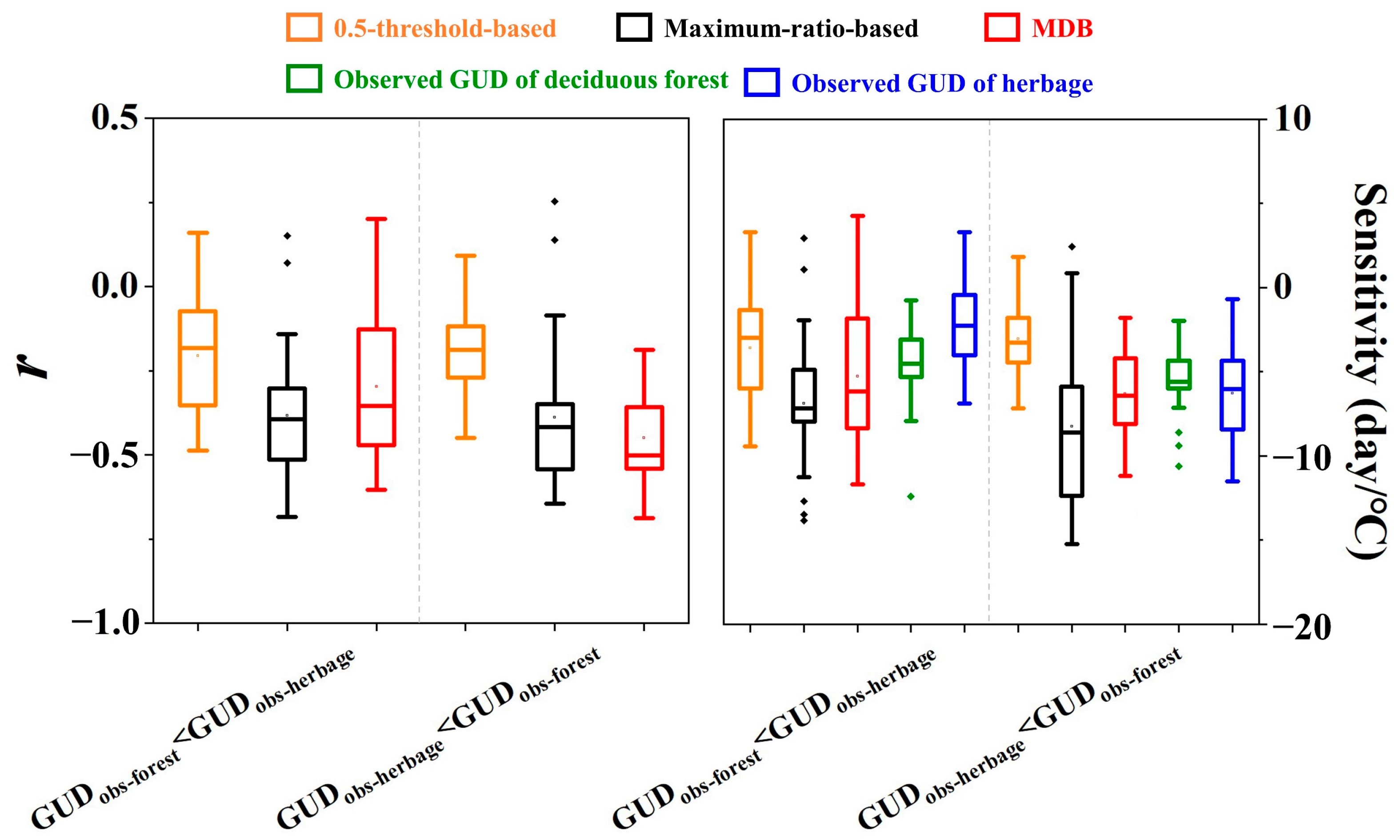
3.2. Climate Factors Sensitivity of Observed GUD

To explore the sensitivity of observed vegetation GUD to climate factors gradients, we acquired the GUDs of deciduous forest and herbages from all the FHM sites in each observed year and plotted them along with the annual mean temperature (Figure 4) and annual precipitation (Figure S3), respectively. Temperature and precipitation are always considered the major driving factors for the spatial and temporal patterns of GUD in temperate regions. However, our results show that the GUD_obs of deciduous forests and herbages were all found earlier with higher temperatures, with correlation coefficients (r) of 0.53 and 0.44 (p < 0.001) for FHM sites with GUD_obs-forest < GUD_obs-herbage, 0.50 and 0.51 (p < 0.001) for FHM sites with GUD_obs-herbage < GUD_obs-forest, respectively. However, these significant negative correlations could be different between deciduous forests and herbages and even their sequential order of green-up onset date. On one hand, the GUDs of deciduous forest would advance by about 4.54 ± 0.38 days/°C, while the GUDs of herbages would advance by over 2.35 ± 0.46 days/°C for FHM sites with GUD_obs-forest < GUD_obs-herbage. On the other hand, observed GUDs also showed significant negative relationships with annual temperature for both vegetation types in FHM sites with GUD_obs-herbage < GUD_obs-forest, and about 5.61 ± 0.35 and 6.29 ± 0.54-day advancement along with 1 °C increase in spring green-up onset for deciduous forest and herbages, respectively. In addition, no significant changes were found in the GUDs of deciduous forests and herbages along the annual precipitation gradient (Figure S3). This indicates that GUDs of deciduous forest and herbages may be more sensitive to annual mean temperature than annual precipitation, and the asynchronization of GUDs between these two vegetation types show an increasing trend as global warming intensifies.

3.3. Comparison and Evaluation among GUD Predictive Methods

GUDs extracted from three turning point identification methods based on a six-degree polynomial function were compared with multi-year ground observation of each FHM site both spatially and temporally. Estimation using the MDB method showed significant relationships (R² = 0.25, p < 0.001) with ground observation in GUDs prediction of deciduous forest (Figure S4c), while all the methods produced a non-significant relationship (p > 0.05) between estimation and ground observation in GUDs prediction of herbages (Figure S4d,e). Results in the above show a significant difference in the GUD between deciduous forests and herbages (Figure 3 and Figure 4). Thus, the magnitude of the difference and even the sequential order of the vegetation green-up onset would lead to considerable uncertainty by using satellite-based turning point detection methods for identifying GUD at a FHM site. Here, we evaluated the performance of three predictive methods by comparing the spatial and temporal variability of estimated GUD with ground observed GUD through all FHM sites.

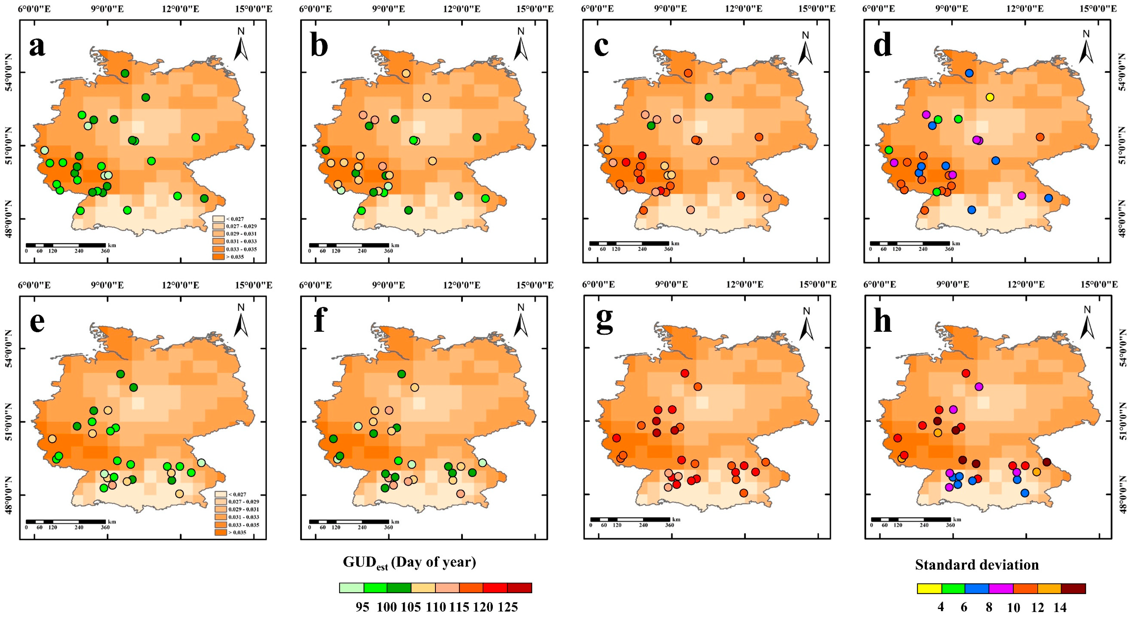
3.3.1. Evaluation on the Spatial Variations of GUD

Results showed that the 0.5-threshold-based method explained poorly the spatial variations of GUD when compared to observations of deciduous forests and herbages at all FHM sites (Figure 5a,d,g,j). For the sites with the GUD of deciduous forest earlier than herbage, GUD derived using the Maximum-ratio-based method showed the highest correlation with ground observed GUDs of forest (R² = 0.26, RMSE = 6.34) (Figure 5b). For the mean absolute difference (MAD) between observed and estimated GUD (|GUD_obs−GUD_est|), the Maximum-ratio-based method also produced lower values (5.02 ± 0.50) than the MDB method (6.64 ± 0.63) (

Table 1. Mean absolute differences between observed GUD of deciduous forest and herbage, and estimated GUD (|GUD_obs − GUD_est|) (Mean ± SE) derived from three predicted methods.

	Site Type	Vegetation Type	0.5-Threshold-Based Method		Maximum-Ratio-Based Method		MDB Method
			Mean	SE	Mean	SE	Mean	SE
Spatial |GUDobs − GUDest|	F < H	DF	9.00	0.53	5.02	0.50	6.64	0.63
		HE	20.13	0.73	14.99	0.72	5.92	0.47
	H < F	DF	18.06	0.79	14.95	0.97	2.79	0.24
		HE	7.64	0.65	5.84	0.63	13.43	0.41
Temporal |GUDobs − GUDest|	F < H	DF	13.40	0.21	9.65	0.18	12.04	0.23
		HE	21.67	0.29	16.90	0.27	9.24	0.22
	H < F	DF	19.45	0.29	16.92	0.31	5.84	0.15
		HE	12.81	0.22	10.52	0.25	14.13	0.23

F < H, FHM sites with GUD_obs-forest < GUD_obs-herbage; H < F, FHM sites with GUD_obs-herbage < GUD_obs-forest; DF, Deciduous Forest; HE, Herbage; MDB method, Maximum-derivative-based method.

, Figure S5a). Contrarily, the MDB method explained relatively higher observed GUDs of herbages compared to the Maximum-ratio-based method, with RMSEs of 6.96 (R² = 0.29, MAD = 5.92 ± 0.47) and 16.01 (R² = 0.10, MAD = 14.99 ± 0.72), respectively (Table 1, Figure 5e,f). For the sites with GUDs of herbage earlier than deciduous forest, however, the MDB method can better explain the spatial variations of GUD compared to the observation of deciduous forest (R² = 0.79, RMSE = 3.25, MAD = 2.79 ± 0.24), whereas the Maximum-ratio-based method performed better for identifying GUDs of herbage (R² = 0.56, RMSE = 7.37, MAD = 5.84 ± 0.63) (Table 1, Figure 5i,k). We also discovered that significant variation in GUD_est between the three methods always occurred in the region with annual mean temperature having a higher increasing trend over the 32-year study periods (Figure 6d,h).

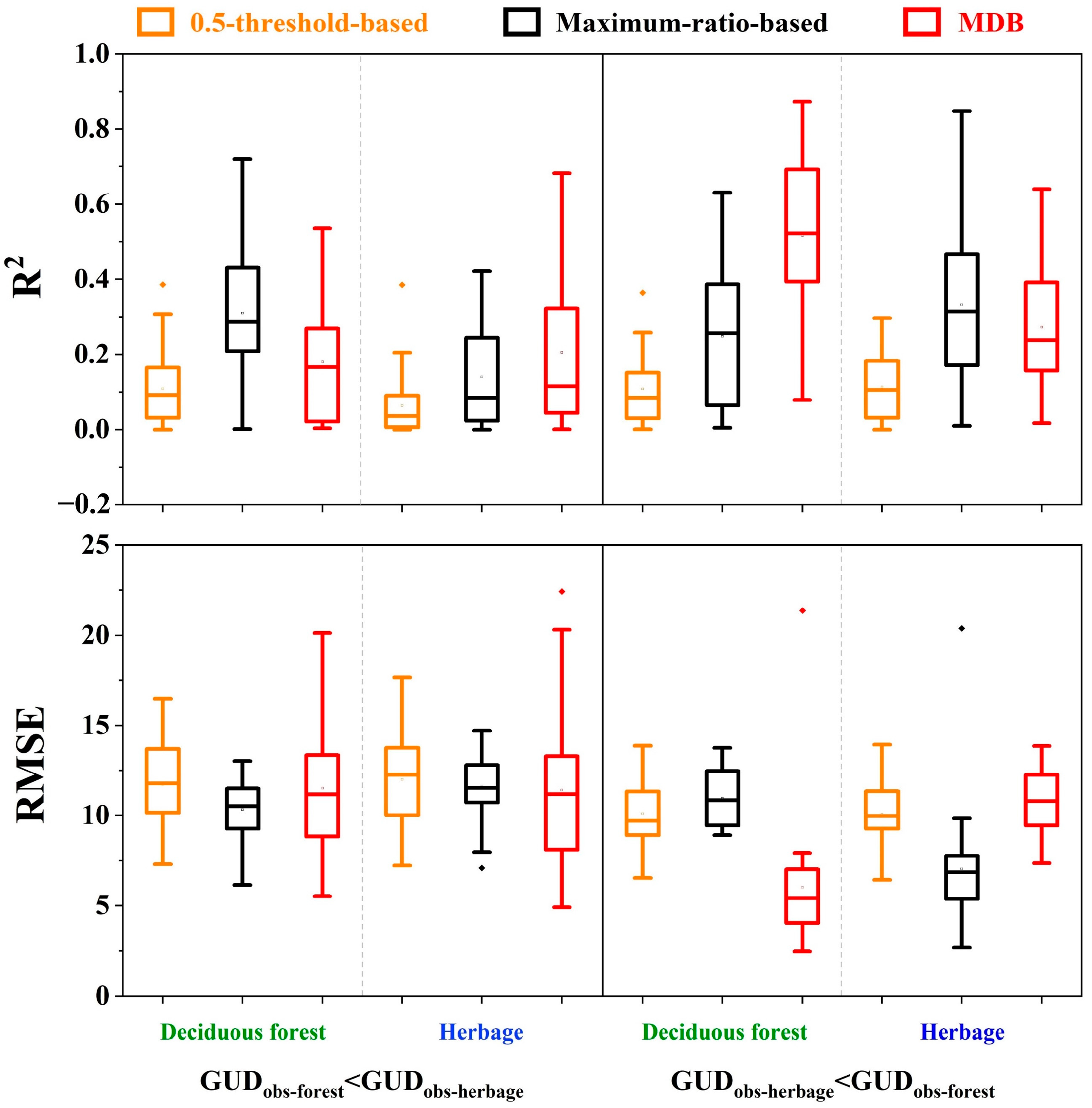
3.3.2. Evaluation on the Temporal Variances of GUD

We also evaluated the estimation performance of three methods for identifying interannual variation in GUDs at all FHM sites with more than 25 years of ground observational data. For the sites with the GUDs of deciduous forest earlier than herbage, similarly, Maximum-ratio-based method showed better performance for identifying GUD of deciduous forest among the three predicted methods, with an R² of 0.24 and RMSE of 12.09 (Figure 7b and Figure 8). However, three predicted methods poorly explained the temporal variations of GUD of herbage and showed low correlations with R² ranging from 0.02 to 0.11 (Figure 7d–f). However, for sites with GUDs of herbage earlier than deciduous forest, the MDB method outperformed the other two methods in identifying GUDs of deciduous forest (Figure 7 and Figure S5). It is notable that predicted results derived from the 0.5-threshold-based method and the Maximum-ratio-based method tended to give earlier GUD compared with ground observations of deciduous forest, while the slopes of the regression line derived from the MDB method were closer to 1 (Figure 7g–i), which indicated that the new method shows better performance than traditional methods for identifying GUD of deciduous forest when the green-up onset of herbage occurs earlier. On the other hand, Maximum-ratio-based method also showed better performance for identifying GUDs of herbage, with an R² of 0.30 and RMSE of 14.15 (Figure 7 and Figure 8).

In addition, we also evaluated the performance of estimated GUD temperature sensitivity identified by the three predictive methods at each FHM site. The three methods showed poor performance in reconstituting the sensitivities to annual mean temperature compared with ground observed GUD of deciduous forest and herbage at sites with the GUD of deciduous forest earlier than herbage (Figure 9). However, the MDB method showed the best performance in reproducing the temperature sensitivity of GUD compared to the observed range at the sites with the GUDs of herbage earlier than deciduous forest (Figure 9).

4. Discussion

The spring vegetation phenology (e.g., GUD) of forests has strong control over carbon capture and storage, and even plays an important role in the productivity and nutrient cycling in terrestrial ecosystems [40,48,49]. Therefore, accurate estimation of regional or global forest phenology has become an urgently needed task for better understanding carbon exchange in the context of global warming, especially because a mismatch in previously synchronized phenological cycles could lead to inaccurate estimates of plant productivity or carbon sequestration [19,50,51]. Using satellite-derived time-series vegetation indices (e.g., NDVI) to predict plant phenology and linking it with environmental and climate variables over regional and global scales has been the primary method for phenological research in recent years. However, it is important to note that large uncertainties still occurred in the predicted GUD using the traditional satellite-derived methods over an ecoregion mixed with different vegetation types (e.g., a site mixed with deciduous forests and herbages in our study). Our analysis found that the GUDs derived from traditional methods, including the 0.5-threshold-based method and the Maximum-ratio-based method, were much less correlated with ground observations of the subsequent-green-up vegetation (Figure 5 and Figure 7). One reason for such uncertainties could be that a satellite vegetation index potentially represents a greenness mixture of different vegetation types, which might have asynchronous GUD [29,42]. That is, it is unclear which leaf emergence in the heterogeneous ecoregion corresponds to a change in the satellite-derived NDVI, and the NDVI time-series dataset frequently shows a rather low temporal resolution with an irregular increase from minimum to maximum values but no notable turn in the reconstructed curve [39,52,53]. It therefore makes it challenging for us to use an absolute NDVI threshold value or a simple maximum change ratio of NDVI time series for the annual onset date of green-up identification [39].

Another possible reason for such poor performance might be the inaccuracy in estimating the phenological transition point in spring. Estimating the turning point from satellite-derived NDVI time series using appropriate methods is an important step in determining the accuracy of the predicted green-up date [29,54]. Results showed that the GUDs derived from the 0.5-threshold-based method were mainly related to the maximum and minimum NDVI values of the entire year Equation (2). Therefore, the premise for applying this method is that the daily NDVI values should be interpolated by a reconstructed growth curve with the daily temporal resolution. However, focusing on temporal resolution may result in over-fitting of the growth curve, leading to unrealistic turning point identification [19]. The other limitation of this method is that the NDVI absolute threshold values always show a departure from reality. Previous studies have confirmed that changes in geographical and meteorological factors (e.g., latitude zones; elevation; hydrologic cycle, rainfall anomaly, etc.) would have a significant effect on different vegetation growth and the annual NDVI peak values [5,15,55,56]. Our study indicated that the Maximum-ratio-based method, which mainly focuses on the changing ratio in the NDVI time series, showed a relatively better performance for reproducing the spatial and temporal variabilities of GUDs of the headmost-green-up vegetation among the three predictive methods (Figure 5 and Figure 7). However, the maximum rate calculated by this method is mainly based on the original temporal resolution (e.g., biweekly NDVI values) by multi-year mean values [16]. Even if the temporal resolution is increased, fluctuations will still occur in the annual NDVI time series due to the asynchronous phenology between deciduous forests and the adjacent and understory herbaceous species [39,40], and each fluctuation will generate a disturbance of changing ratio, which might be potentially misidentified as the turning point of GUD.

We developed and applied a new MDB method to identify the turning point and predicted the GUDs of subsequent-green-up vegetation types, especially in the FHM sites, with GUD_obs-herbage < GUD_obs-forest. Results showed that the predicted green-up dates based on the new MDB method are generally matched to the ground observations in the FHM sites with GUDs of herbage earlier than in deciduous forest. This new method takes account of the interannual variation and temporal resolution (i.e., daily), and more importantly, it improves the identification of the turning point threshold when deciduous forests start to green up after herbaceous cover by integrating the first and second derivatives of the curve function. This makes the new method largely different from the two traditional methods. Instead of using the NDVI time series at the original biweekly temporal resolution by the Maximum-ratio-based method, the MDB method uses the sixth-degree polynomial function to drive the daily interpolated NDVI values for threshold determination by fitting the 32-year mean NDVI time series at each FHM site. In addition, asynchronous phenological onset date errors derived by advanced GUD of herbage and mixed-greenness effects all existed in the two traditional methods. These issues were considered in the MDB method by calculating the first and second derivatives of the fitting curve function, which improved the accuracy of inflection point detection on a secondary change in greenness within a given pixel and allowed a relatively good match between NDVI threshold and the corresponding green-up date of subsequent-green-up vegetation type.

Many previous studies have found an earlier spring phenology in response to global warming [26,34,57]. Temperature is the main driver of vegetation growth, and in many cases rising temperatures have been proved to accelerate vegetation growth and result in an earlier arrival at the next phenological phase [58,59]. Different views also expressed that a delayed onset of spring grassland phenology also occurred, and geographical or hydrometeorological factors can certainly be recognized as the dominant factor rather than temperature increment [4]. However, our study confirmed that the interannual precipitation did not affect the variability of GUD but it showed a significant negative trend with the annual mean temperature (p < 0.05) for both deciduous forests and herbages (Figure 4). Interannual analysis also showed a significant advanced trend of GUD_obs both for deciduous forest and herbages (Figure 3). The above results have implied that higher annual mean temperature would advance the GUDs of deciduous forest and herbage, but it should be noticed that different vegetation types have inconsistent sensitive trends to annual mean temperature in the same FHM site. Significant deviation in predicted results between the three methods were observed as temperatures rose (Figure 6), indicating that the asynchronous phenological phases between deciduous forests and herbages would become more pronounced, making it more difficult to identify the GUD in a given pixel and scale up plant phenology from species to ecoregion level in the context of global warming [17,60].

5. Conclusions

Unsatisfactory accuracy of satellite-based methods in identifying GUDs within a heterogeneous ecoregion, caused primarily by mixed greenness and asynchronous vegetation phenological phases, might induce considerable uncertainties when predicting vegetation phenological responses to future climate change, and thereby also in the simulations of terrestrial water, energy, and carbon balance [17,40,61]. The critical step in predicting the GUD is determining the onset date of the inflection point using either a predetermined threshold or a change ratio [62]. Based on the precondition that the predicted ecoregion is mainly covered with deciduous forests and herbages. We developed a new inflection point identifying method (the MDB method) and then provided inter-comparisons between the MDB method and the traditional methods with ground-observed GUDs of deciduous forest and herbages. Traditional methods for detecting the onset date of infection point and thereby the GUD prediction from the GIMMS NDVI3g time series are not sufficiently flexible or accurate. Our comparisons showed that the MDB method outperformed the other two traditional methods in estimating the GUD of deciduous forest when it was later than that of herbage. However, there remain some uncertainties in the new MDB method that should be considered.

One concern is that the coarse spatial and temporal resolutions could inevitably reduce the accuracy in identifying the vegetation phenological phases. In this study, we have selected the ideal sites mainly covered with deciduous forest and herbages beforehand, and the onset date of green up in herbages is earlier or later than that of deciduous forests, which is known in advance. However, in many cases, more than two species are present in the same ecoregion, which means that the GUD estimated by the new improved method might be ineffective for such complex scenes [63]. Consequently, there would be an urgent need for reasonable methods to discriminate among different spring phenological phases for different vegetation types by reconstructing the time-series dataset of vegetation indices with finer spatial-temporal resolution. Further studies about the preferable satellite-derived vegetation indices (e.g., enhanced vegetation index (EVI), Medium Resolution Imaging Spectrometer Terrestrial Chlorophyll index (MTCI), etc.) and reasonable fitting models for time-series vegetation index smoothing should be conducted in future phenological research [29,51].

Another concern is that the empirical statistical relationships simply analyze the underlying mechanistic processes governing plant spring green-up date. The onset of spring vegetation green up has been confirmed to be correlated with annual temperature [64,65,66]. Our results also found that the green-up dates of both deciduous forests and herbages have a significant relationship with annual air temperature (Figure 4), yet these relationships vary largely across different ecoregions and vegetation types. Previous studies have found that the temperature sensitivity of spring phenology in temperate forests has decreased along with the climate warming over Europe [63]. This is primarily due to the complex interaction of environmental factors and temperature, as well as the insufficient chilling caused by the associated winter warming [67,68]. Consequently, understanding of how climate warming interacts with other factors, such as photoperiod, precipitation, drought, and so on, and the underlying mechanisms might enhance our capacity to predict plant phenological phase changes over an ecoregion-scale under future, ongoing climate warming.

Our study highlights the limitation of current inflection point identification algorithms in predicting the GUD inferred from satellite-derived vegetation indexes time series in an ecoregion with heterogeneous vegetation types and asynchronous phenological phases, as well as suggesting the importance of applying appropriate methods for larger-scale spring phenology events reproducing with consideration of the asynchronization of onset dates both in different vegetation types and species.

References

1. Barr, A.G.; Black, T.A.; Hogg, E.H.; Griffis, T.J.; Morgenstern, K.; Kljun, N.; Theede, A.; Nesic, Z. Climate controls on the carbon and water balances of a boreal aspen forest, 1994–2003. Glob. Chang. Biol. 2007, 13, 561–576. [Google Scholar] [CrossRef]
2. Ganguly, S.; Friedl, M.A.; Tan, B.; Zhang, X.; Verma, M. Land surface phenology from MODIS: Characterization of the Collection 5 global land cover dynamics product. Remote Sens. Environ. 2010, 114, 1805–1816. [Google Scholar] [CrossRef]
3. Wu, C.Y.; Hou, X.H.; Peng, D.L.; Gonsamo, A.; Xu, S.G. Land surface phenology of China’s temperate ecosystems over 1999–2013: Spatial-temporal patterns, interaction effects, covariation with climate and implications for productivity. Agric. Forest Meteorol. 2016, 216, 177–187. [Google Scholar] [CrossRef]
4. Rajan, H.; Jeganathan, C. Understanding Spatio-temporal Pattern of Grassland Phenology in the western Indian Himalayan State. J. Indian Soc. Remote 2019, 47, 1137–1151. [Google Scholar] [CrossRef]
5. Singh, B.; Jeganathan, C.; Rathore, V.S. Improved NDVI based proxy leaf-fall indicator to assess rainfall sensitivity of deciduousness in the central Indian forests through remote sensing. Sci. Rep. 2020, 10, 17638. [Google Scholar] [CrossRef]
6. Liu, Z.J.; Wu, C.Y.; Liu, Y.S.; Wang, X.; Fang, B.; Yuan, W.; Ge, Q. Spring green-up date derived from GIMMS3g and SPOT-VGT NDVI of winter wheat cropland in the North China Plain. ISPRS J. Photogram. Remote Sens. 2017, 130, 81–91. [Google Scholar] [CrossRef]
7. Richardson, A.D.; Keenan, T.F.; Migliavacca, M.; Ryu, Y.; Sonnentag, O.; Toomey, M. Climate change, phenology, and phenological control of vegetation feedbacks to the climate system. Agric. Forest Meteorol. 2013, 169, 156–173. [Google Scholar] [CrossRef]
8. Wang, L.; De Boeck, H.J.; Chen, L.; Song, C.; Chen, Z.; McNulty, S.; Zhang, Z. Urban warming increases the temperature sensitivity of spring vegetation phenology at 292 cities across China. Sci. Total Environ. 2022, 834, 155154. [Google Scholar] [CrossRef]
9. Piao, S.; Tan, J.; Chen, A.; Fu, Y.H.; Ciais, P.; Liu, Q.; Janssens, I.A.; Vicca, S.; Zeng, Z.; Jeong, S.J.; et al. Leaf onset in the northern hemisphere triggered by daytime temperature. Nat. Commum. 2015, 6, 6911. [Google Scholar] [CrossRef]
10. Piao, S.; Wang, X.; Ciais, P.; Zhu, B.; Wang, T.; Liu, J. Changes in satellite-derived vegetation growth trend in temperate and boreal Eurasia from 1982 to 2006. Glob. Chang. Biol. 2011, 17, 3228–3239. [Google Scholar] [CrossRef]
11. Barichivich, J.; Briffa, K.R.; Myneni, R.B.; Osborn, T.J.; Melvin, T.M.; Ciais, P.; Piao, S.; Tucker, C. Large-scale variations in the vegetation growing season and annual cycle of atmospheric CO2. Glob. Chang. Biol. 2013, 19, 3167–3183. [Google Scholar] [CrossRef] [PubMed]
12. Piao, S.; Ciais, P.; Friedlingstein, P.; Peylin, P.; Reichstein, M.; Luyssaert, L.; Margolis, H.; Fang, J.; Barr, A.; Chen, A.; et al. Net carbon dioxide losses of northern ecosystems in response to autumn warming. Nature 2008, 451, 49–52. [Google Scholar] [CrossRef]
13. Keenan, T.F.; Gray, J.; Friedl, M.A.; Toomey, M.; Bohrer, G.; Hollinger, D.Y.; Munger, J.W.; O’Keefe, J.; Schmid, H.P.; Wing, I.S.; et al. Net carbon uptake has increased through warming-induced changes in temperate forest phenology. Nat. Clim. Chang. 2014, 4, 598–604. [Google Scholar] [CrossRef]
14. Zeng, Z.; Piao, S.; Li, L.Z.X.; Zhou, L.; Ciais, P.; Wang, T.; Li, Y.; Lian, X.; Wood, E.F.; Friedlingstein, P.; et al. Climate mitigation from vegetation biophysical feedbacks during the past three decades. Nat. Clim. Chang. 2017, 7, 432–436. [Google Scholar] [CrossRef]
15. Shen, R.; Chen, X.; Chen, L.; He, B.; Yuan, W. Regional evaluation of satellite-based methods for identifying leaf unfolding date. ISPRS J. Photogram. Remote Sens. 2021, 175, 88–98. [Google Scholar] [CrossRef]
16. Piao, S.; Fang, J.; Zhou, L.; Ciais, P.; Zhu, B. Variations in satellite-derived phenology in China’s temperate vegetation. Glob. Chang. Biol. 2006, 12, 672–685. [Google Scholar] [CrossRef]
17. Piao, S.; Liu, Q.; Chen, A.; Janssens, I.A.; Fu, Y.; Dai, J.; Liu, L.; Lian, X.; Shen, M.; Zhu, Z. Plant phenology and global climate change: Current progresses and challenges. Glob. Chang. Biol. 2019, 25, 1922–1940. [Google Scholar] [CrossRef]
18. Reed, B.C.; Brown, J.F.; VanderZee, D.; Loveland, T.R.; Merchant, J.W.; Ohlen, D. Measuring phenological variability from satellite imagery. J. Veg. Sci. 1994, 5, 703–714. [Google Scholar] [CrossRef]
19. Wu, C.Y.; Peng, D.L.; Soudani, K.; Siebicke, L.; Gough, C.M.; Arain, M.A.; Bohrer, G.; Lafleur, P.M.; Peichl, M.; Gonsamo, A.; et al. Land surface phenology derived from normalized difference vegetation index (NDVI) at global FLUXNET sites. Agric. For. Meteorol. 2017, 233, 171–182. [Google Scholar] [CrossRef]
20. Heck, E.; de Beurs, K.M.; Owsley, B.C.; Henebry, G.M. Evaluation of the MODIS collections 5 and 6 for change analysis of vegetation and land surface temperature dynamics in North and South America. ISPRS J. Photogram. Remote Sens. 2019, 156, 121–134. [Google Scholar] [CrossRef]
21. White, M.A.; de Beurs, K.M.; Didan, K.; Inouye, D.W.; Richardson, A.D.; Jensen, O.P.; O’Keefe, J.; Zhang, G.; Nemani, R.R.; Van Leeuwen, W.J.D.; et al. Intercomparison, interpretation, and assessment of spring phenology in North America estimated from remote sensing for 1982–2006. Glob. Chang. Biol. 2009, 15, 2335–2359. [Google Scholar] [CrossRef]
22. Friedl, M.A.; Gray, J.M.; Melaas, E.K.; Richardson, A.D.; Hufkens, K.; Keenan, T.F.; Bailey, A.; O’Keefe, J. A tale of two springs: Using recent climate anomalies to characterize the sensitivity of temperate forest phenology to climate change. Environ. Res. Lett. 2014, 9, 054006. [Google Scholar] [CrossRef]
23. Peng, D.L.; Wu, C.Y.; Li, C.J.; Zhang, X.; Liu, Z.; Ye, H.; Luo, S.; Liu, X.; Hu, Y.; Fang, B. Spring green-up phenology products derived from MODIS NDVI and EVI: Intercomparison, interpretation and validation using National Phenology Network and AmeriFlux observations. Ecol. Indic. 2017, 77, 323–336. [Google Scholar] [CrossRef]
24. Chen, J.; Jönsson, P.; Tamura, M.; Gu, Z.; Matsushita, B.; Eklundh, L. A simple method for reconstructing a high-quality NDVI time-series data set based on the Savitzky-Golay filter. Remote Sens. Environ. 2004, 91, 332–344. [Google Scholar] [CrossRef]
25. Cong, N.; Piao, S.; Chen, A.; Wang, X.; Lin, X.; Chen, S.; Han, S.; Zhou, G.; Zhang, X. Spring vegetation green-up date in China inferred from SPOT NDVI data: A multiple model analysis. Agric. For. Meteorol. 2012, 165, 104–113. [Google Scholar] [CrossRef]
26. Wang, J.; Wu, C.; Wang, X.; Zhang, X. A new algorithm for the estimation of leaf unfolding date using MODIS data over China’s terrestrial ecosystems. ISPRS J. Photogram. Remote Sens. 2019, 149, 77–90. [Google Scholar] [CrossRef]
27. Cao, R.; Chen, Y.; Shen, M.; Chen, J.; Zhou, J.; Wang, C.; Yang, W. A simple method to improve the quality of NDVI time-series data by integrating spatiotemporal information with the Savitzky-Golay filter. Remote Sens. Environ. 2018, 217, 244–257. [Google Scholar] [CrossRef]
28. Li, Y.; Zhang, Y.; Gu, F.; Liu, S. Discrepancies in vegetation phenology trends and shift patterns in different climatic zones in middle and eastern Eurasia between 1982 and 2015. Ecol. Evol. 2019, 9, 8664–8675. [Google Scholar] [CrossRef]
29. Cao, R.; Chen, J.; Shen, M.; Tang, Y. An improved logistic method for detecting spring vegetation phenology in grasslands from MODIS EVI time-series data. Agric. Forest Meteorol. 2015, 200, 9–20. [Google Scholar] [CrossRef]
30. Yu, H.Y.; Luedeling, E.; Xu, J.C. Winter and spring warming result in delayed spring phenology on the Tibetan Plateau. Proc. Natl. Acad. Sci. USA 2010, 107, 22151–22156. [Google Scholar] [CrossRef] [Green Version]
31. Lloyd, D. A phenological classification of terrestrial vegetation cover using shortwave vegetation index imagery. Int. J. Remote Sens. 1990, 11, 2269–2279. [Google Scholar] [CrossRef]
32. Suzuki, R.; Nomaki, T.; Yasunari, T. West–east contrast of phenology and climate in northern Asia revealed using a remotely sensed vegetation index. Int. J. Biometeorol. 2003, 47, 126–138. [Google Scholar] [CrossRef] [PubMed]
33. Yu, S.; Xia, J.; Yan, Z.; Yang, K. Changing spring phenology dates in the Three-Rivers Headwater Region of the Tibetan Plateau during 1960–2013. Adv. Atmos. Sci. 2018, 35, 116–126. [Google Scholar] [CrossRef]
34. Buitenwerf, R.; Rose, L.; Higgins, S. Three decades of multi-dimensional change in global leaf phenology. Nat. Clim. Chang. 2015, 5, 364–368. [Google Scholar] [CrossRef]
35. Shen, M.; Zhang, G.; Cong, N.; Wang, S.; Kong, W.; Piao, S. Increasing altitudinal gradient of spring vegetation phenology during the last decade on the Qinghai-Tibetan Plateau. Agric. For. Meteorol. 2014, 189, 71–80. [Google Scholar] [CrossRef]
36. White, M.A.; Thornton, P.E.; Running, S.W. A continental phenology model for monitoring vegetation responses to interannual climatic variability. Glob. Biogeochem. Cycles 1997, 11, 217–234. [Google Scholar] [CrossRef]
37. Chen, X.; Wang, D.; Chen, J.; Wang, C.; Shen, M. The mixed pixel effect in land surface phenology: A simulation study. Remote Sens. Environ. 2018, 211, 338–344. [Google Scholar] [CrossRef]
38. Liu, L.; Cao, R.; Shen, M.; Chen, J.; Wang, J.; Zhang, X. How dose scale effect influence spring vegetation phenology estimated from satellite-derived vegetation indexes? Remote Sens. 2019, 11, 2137. [Google Scholar] [CrossRef]
39. Badeck, F.W.; Bondeau, A.; Böttcher, K.; Doktor, D.; Lucht, W.; Schaber, J.; Sitch, S. Responses of spring phenology to climate change. New Phytol. 2004, 162, 295–309. [Google Scholar] [CrossRef]
40. Fridley, J.D. Extended leaf phenology and the autumn niche in deciduous forest invasions. Nature 2012, 485, 359–362. [Google Scholar] [CrossRef]
41. Augspurger, C.K.; Cheeseman, J.M.; Salk, C.F. Light gains and physiological capacity of understory woody plants during phenological avoidance of canopy shade. Funct. Ecol. 2005, 19, 537–547. [Google Scholar] [CrossRef]
42. Richardson, A.D.; O’Keefe, J. Phenological differences between understory and overstory: A case study using the long-term Harvard Forest records. In Phenology of Ecosystem Processes; Noormets, A., Ed.; Springer: New York, NY, USA, 2009; pp. 87–117. [Google Scholar]
43. Zhang, X.; Liu, L.; Chen, X.; Gao, Y.; Xie, S.; Mi, J. GLC_FCS30: Global land-cover product with fine classification system at 30 m using time-series Landsat imagery. Earth Syst. Sci. Data 2021, 13, 2753–2776. [Google Scholar] [CrossRef]
44. Sobrino, J.A.; Julien, Y.; Atitar, M.; Nerry, F. NOAA-AVHRR orbital drift correction from solar zenithal angle data. IEEE Trans. Geosci. Remote 2008, 46, 4014–4019. [Google Scholar] [CrossRef]
45. Wang, J.; Wu, C.Y.; Zhang, C.H.; Ju, W.; Wang, X.; Chen, Z.; Fang, B. Improved modeling of gross primary productivity (GPP) by better representation of plant phenological indicators from remote sensing using a process model. Ecol. Ind. 2018, 88, 332–340. [Google Scholar] [CrossRef]
46. Viovy, N. CRUNCEP Version 7-Atmospheric Forcing Data for the Community Land Model; Research Data Archive at the National Center for Atmospheric Research, Computational and Information Systems Laboratory: Boulder, CO, USA, 2018. [Google Scholar] [CrossRef]
47. Zhu, L.; Meng, J. Determining the relative importance of climatic drivers on spring phenology in grassland ecosystems of semi-arid areas. Int. J. Biometeorol. 2014, 59, 237–248. [Google Scholar] [CrossRef]
48. Polgar, C.A.; Primack, R.B. Leaf-out phenology of temperate woody plants: From trees to ecosystems. New Phytol. 2011, 191, 926–941. [Google Scholar] [CrossRef]
49. Richardson, A.D.; Black, T.A.; Ciais, P.; Delbart, N.; Friedl, M.A.; Gobron, N.; Hollinger, D.Y.; Kutsch, W.L.; Longdoz, B.; Luyssaet, S.; et al. Influence of spring and autumn phenological transitions on forest ecosystem productivity. Phil. Trans. R. Soc. B. 2010, 365, 3227–3246. [Google Scholar] [CrossRef]
50. Morisette, J.T.; Richardson, A.D.; Knapp, A.K.; Fisher, J.I.; Graham, E.A.; Abatzoglou, J.; Wilson, B.E.; Breshears, D.D.; Henebry, G.M.; Hanes, J.M.; et al. Tracking the rhythm of the seasons in the face of global change: Phenological research in the 21st century. Front. Ecol. Environ. 2009, 7, 253–260. [Google Scholar] [CrossRef]
51. Atkinson, P.M.; Jeganathan, C.; Dash, J.; Dash, J.; Atzberger, C. Inter-comparison of four models for smoothing satellite sensor time-series data to estimate vegetation phenology. Remote Sen. Environ. 2012, 123, 400–417. [Google Scholar] [CrossRef]
52. Chen, X.Q.; Pan, W.F. Relationships among phenological growing season, time-integrated normalized difference vegetation index and climate forcing in the temperate region of eastern China. Int. J. Climatol. 2002, 22, 1781–1792. [Google Scholar] [CrossRef]
53. Fisher, J.I.; Richardson, A.D.; Mustard, J.F. Phenology model from surface meteorology does not capture satellite-based greenup estimations. Global Chang. Biol. 2007, 13, 707–721. [Google Scholar] [CrossRef]
54. Fisher, J.I.; Mustard, J.F. Cross-scalar satellite phenology from ground, Landsat, and MODIS data. Remote Sens. Environ. 2007, 109, 261–273. [Google Scholar] [CrossRef]
55. Yuan, W.; Zheng, Y.; Piao, S.; Ciais, P.; Lombardozzi, D.; Wang, Y.; Ryu, Y.; Chen, G.; Dong, W.; Hu, Z.; et al. Increased atmospheric vapor pressure deficit reduces global vegetation growth. Sci. Adv. 2019, 5, eaax1396. [Google Scholar] [CrossRef]
56. Jeganathan, C.; Dash, J.; Atkinson, P.M. Remotely sensed trends in the phenology of northern high latitude terrestrial vegetation, controlling for land cover change and vegetation type. Remote Sen. Environ. 2014, 143, 154–170. [Google Scholar] [CrossRef]
57. Chuine, I.; Morin, X.; Bugmann, H. Warming, photoperiods, and tree phenology. Science 2010, 329, 277–278. [Google Scholar] [CrossRef]
58. Cleland, E.E.; Chuine, I.; Menzel, A.; Mooney, H.A.; Schwartz, M.D. Shifting plant phenology in response to global change. Trends Ecol. Evol. 2007, 22, 357–365. [Google Scholar] [CrossRef]
59. Kobayashi, H.; Yunus, A.P.; Nagai, S.; Sugiura, K.; Kim, Y.; Van Dam, B.; Nagano, H.; Zona, D.; Harazono, Y.; Bret-Harte, M.S.; et al. Latitudinal gradient of spruce forest understory and tundra phenology in Alaska as observed from satellite and ground-based data. Remote Sens. Environ. 2016, 177, 160–170. [Google Scholar] [CrossRef]
60. Jeong, S.J.; Schimel, D.; Frankenberg, C.; Drewry, D.T.; Fisher, J.B.; Verma, M.; Berry, J.A.; Lee, J.E.; Joiner, J. Application of satellite solar-induced chlorophyll fluorescence to understanding large-scale variations in vegetation phenology and function over northern high latitude forests. Remote Sens. Environ. 2017, 190, 178–187. [Google Scholar] [CrossRef]
61. Richardson, A.D.; Anderson, R.S.; Arain, A.M.; Barr, A.G.; Bohrer, G.; Chen, G.; Chen, J.M.; Ciais, P.; Davis, K.J.; Desai, A.R.; et al. Terrestrial biosphere models need better representation of vegetation phenology: Results from the North American carbon program site synthesis. Glob. Chang. Biol. 2012, 18, 566–584. [Google Scholar] [CrossRef] [Green Version]
62. Liu, Q.; Fu, Y.H.; Liu, Y.; Janssens, I.A.; Piao, S. Simulating the onset of spring vegetation growth across the Northern Hemisphere. Glob. Chang. Biol. 2018, 24, 1342–1356. [Google Scholar] [CrossRef]
63. Fu, Y.H.; Piao, S.; Zhao, H.; Jeong, S.J.; Wang, X.; Vitasse, Y.; Ciais, P.; Janssens, I.A. Unexpected role of winter precipitation in determining heat requirement for spring vegetation green-up at northern middle and high latitudes. Glob. Chang. Biol. 2014, 20, 3743–3755. [Google Scholar] [CrossRef] [PubMed]
64. Peñuelas, J.; Rutishauser, T.; Filella, I. Phenology feedbacks on climate change. Science 2009, 324, 887–888. [Google Scholar] [CrossRef] [PubMed]
65. Rossi, S.; Isabel, N. Bud break responds more strongly to daytime than night-time temperature under asymmetric experimental warming. Glob. Chang. Biol. 2017, 23, 446–454. [Google Scholar] [CrossRef] [PubMed]
66. Sun, Q.; Li, B.; Jiang, Y.; Chen, X.; Zhou, G. Declined trend in herbaceous plant green-up dates on the Qinghai–Tibetan Plateau caused by spring warming slowdown. Sci. Total Environ. 2021, 772, 145039. [Google Scholar] [CrossRef]
67. Flynn, D.F.B.; Wolkovich, E.M. Temperature and photoperiod drive spring phenology across all species in a temperate forest community. New Phytol. 2018, 219, 1353–1362. [Google Scholar] [CrossRef]
68. Vitasse, Y.; Signarbieux, C.; Fu, Y.H. Global warming leads to more uniform spring phenology across elevations. Proc. Natl. Acad. Sci. USA 2018, 115, 1004–1008. [Google Scholar] [CrossRef] [Green Version]
Figure 1. Multi-years average value of normalized difference vegetation index (NDVI) time-series data and the observed green-up date (GUD) (Green dash line for deciduous forest and blue dash line for herbage, respectively) in site PEP_ID_2672 (a) and site PEP_ID_2879 (b) of the Pan European Phenology (PEP) Database. The red line is the fitted curve based on the six-degree polynomial function (Equation (1)). The frequency histogram (c) shows the multi-year average difference values of observed GUD between deciduous forest (GUDobs-forest) and herbage (GUDobs-herbage) in the selected forest-herbage-mixed (FHM) sites in our study.
Remotesensing 14 04349 g001
Figure 2. The distribution of the forest-herbage-mixed (FHM) sites were obtained from the Pan European Phenology Database (PEP725).
Remotesensing 14 04349 g002
Figure 3. Interannual variation and trends in vegetation green-up dates (GUD) for deciduous forest and herbages, and annual mean temperature from 1982 to 2013 over the selected 58 forest-herbage-mixed (FHM) sites.
Remotesensing 14 04349 g003
Figure 4. Relationships between annual observed green-up dates (GUDobs) of deciduous forest (green) and herbages (blue) and annual mean temperature for all forest-herbage-mixed (FHM) sites with GUDobs-forest < GUDobs-herbage (a) and with GUDobs-herbage < GUDobs-forest (b) The embedded box plots show the correlation coefficients (r) and slope (s) of regression lines, which indicate the change trend of GUD with the increased annual mean temperature for each FHM site.
Remotesensing 14 04349 g004
Figure 5. Comparisons between multi-year average observed green-up dates (GUDobs) of deciduous forest (green) and herbages (blue) and estimated green-up dates (GUDest) of three methods (0.5-threshold-based method, Maximum-ratio-based method, and Maximum-derivative-based (MDB) method) for forest-herbage-mixed (FHM) sites with GUDobs-forest < GUDobs-herbage (af) and with GUDobs-herbage < GUDobs-forest (gl). The gray dashed line represents the 1:1 line, and the red lines are the regression lines. The root mean square error (RMSE) was also used to evaluate the predictive performance.
Remotesensing 14 04349 g005
Figure 6. The spatial distribution of the multi-year average estimated green-up dates (GUDest) of three methods (0.5-threshold-based method, Maximum-ratio-based methods, and Maximum-derivative-based (MDB) method) for forest-herbage-mixed (FHM) sites with GUDobs-forest < GUDobs-herbage (ac) and with GUDobs-herbage < GUDobs-forest (eg), (d,h) show the standard deviation of three methods. Gradients in the base map indicated the increasing trend of annual mean temperature from 1982 to 2013.
Remotesensing 14 04349 g006
Figure 7. Comparisons between annual observed green-up dates (GUDobs) of deciduous forest (green) and herbages (blue) and estimated green-up dates (GUDest) of three methods (0.5-threshold-based method, Maximum-ratio-based method, and Maximum-derivative-based (MDB) method) for forest-herbage-mixed (FHM) sites with GUDobs-forest < GUDobs-herbage (af) and with GUDobs-herbage < GUDobs-forest (gl). The gray dashed line represents the 1:1 line, and the red lines are the regression lines. The root mean square error (RMSE) was also used to evaluate the predictive performance.
Remotesensing 14 04349 g007
Figure 8. Comparisons of three predicted methods (0.5-threshold-based method, Maximum-ratio-based method, and Maximum-derivative-based (MDB) method) for reproducing temporal variations of green-up date (GUD) by using coefficient of determination (R2) and the root mean square error (RMSE) between estimated GUD and observed GUDs of deciduous forest and herbage across all forest-herbage-mixed (FHM) sites with GUDobs-forest < GUDobs-herbage and with GUDobs-herbage < GUDobs-forest.
Remotesensing 14 04349 g008
Figure 9. Sensitivity of estimated green-up date (GUDest) derived from three predictive methods (0.5-threshold-based method, Maximum-ratio-based method, Maximum-derivative-based (MDB) method), and ground observed GUD (GUDobs) of deciduous forest and herbage to annual mean temperature in the forest-herbage-mixed (FHM) sites with GUDobs-forest < GUDobs-herbage and with GUDobs-herbage < GUDobs-forest.
Remotesensing 14 04349 g009