

On the Use of Sentinel-2 NDVI Time Series and Google Earth Engine to Detect Land-Use/Land-Cover Changes in Fire-Affected Areas

 ,
,
Abstract
:1. Introduction
- (i)
- (ii)
- Multi-temporal analysis methods can be split into: (i) temporal segmentation algorithms, such as CCDC (continuous change detection and classification), VERDeT (vegetation regeneration and disturbance estimates through time), and LandTrend [41,42,43,44,45,46,47,48]; and (ii) trend analysis [49,50,51,52,53,54,55,56] to detect land-use/land-cover changes by analyzing the pixel-in-time signal [47,57,58,59,60].
2. Materials and Methods
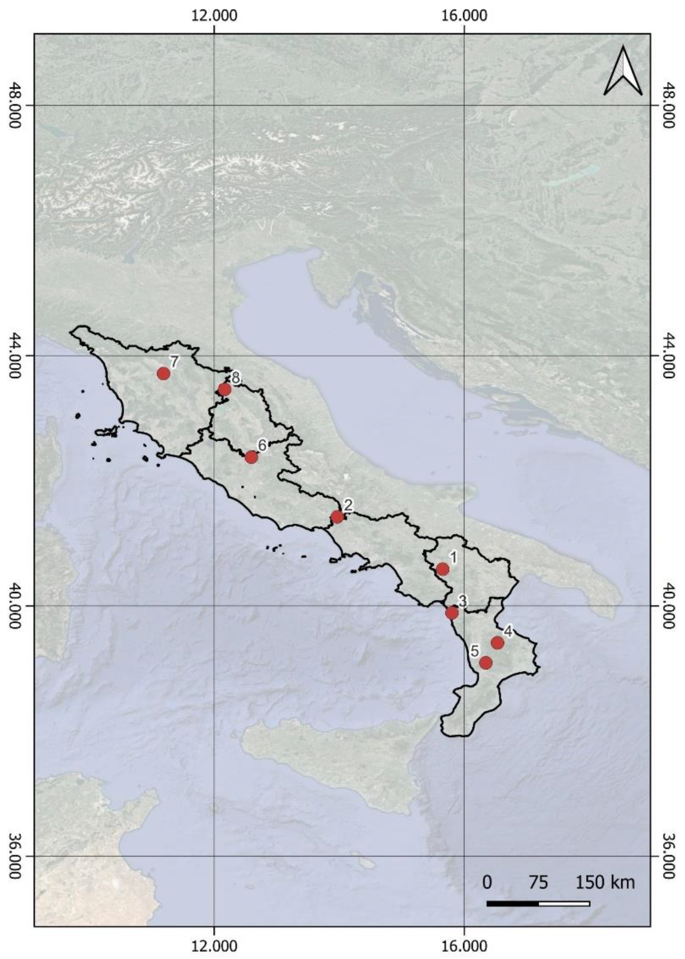
2.1. Study Area
2.2. Methodological Approach Rationale, Tools, and Datasets
- (i)
- What type of data processing can be adopted to suitably transform spectral information into vegetation parameters?
- (ii)
- What is the minimum mapping unit (pixel, cadastral parcel, or segment level) to be considered from satellite Sentinel-2?
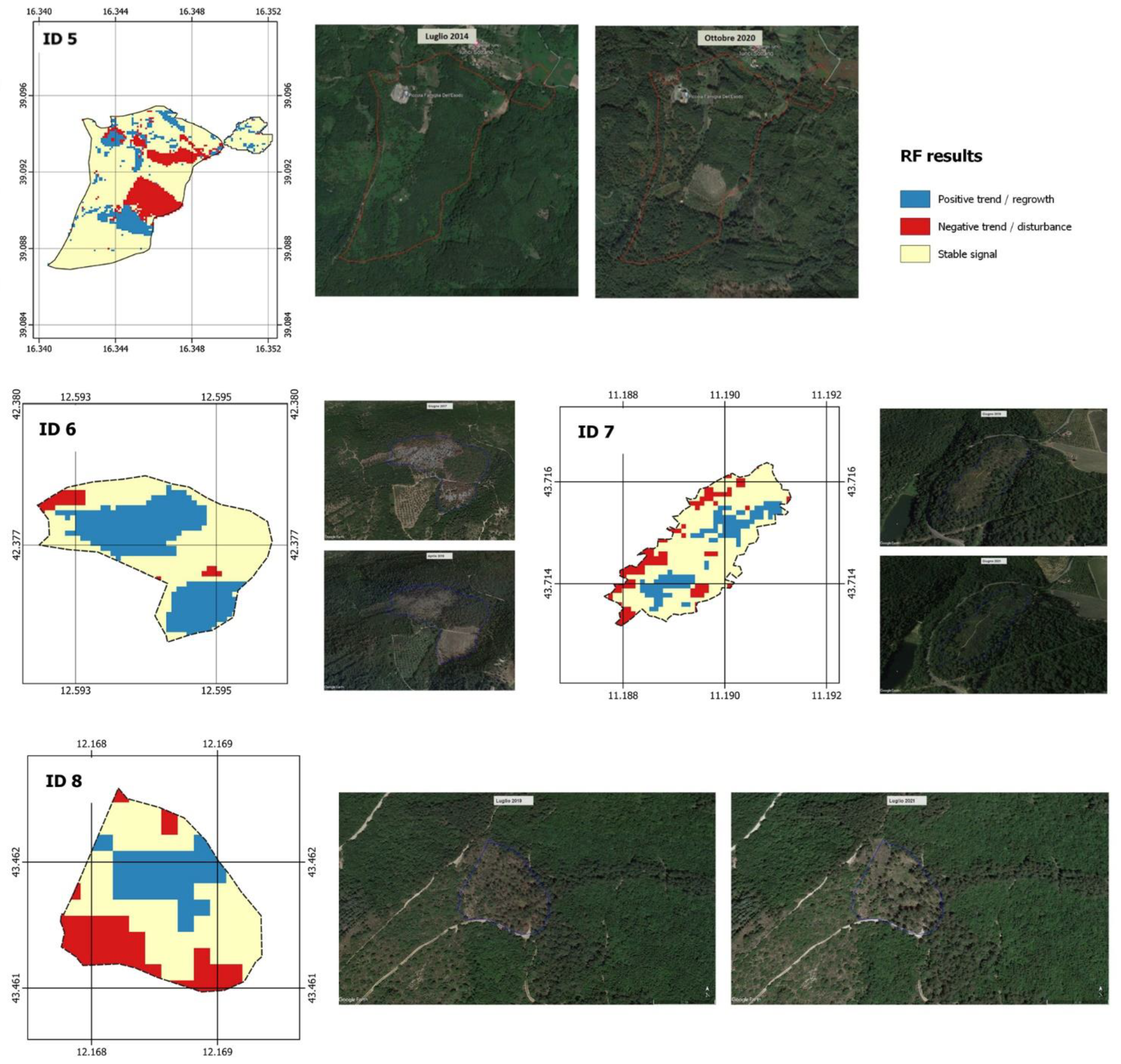
2.3. Methods
3. Results and Discussion
4. Conclusions
Author Contributions
Funding
Data Availability Statement
Acknowledgments
Conflicts of Interest
References
- Hermosilla, T.; Wulder, M.A.; White, J.C.; Coops, N.C.; Hobart, G.W. Disturbance-Informed Annual Land Cover Classification Maps of Canada’s Forested Ecosystems for a 29-Year Landsat Time Series. Can. J. Remote Sens. 2018, 44, 67–87. [Google Scholar] [CrossRef]
- Wulder, M.A.; Loveland, T.R.; Roy, D.P.; Crawford, C.J.; Masek, J.G.; Woodcock, C.E.; Allen, R.G.; Anderson, M.C.; Belward, A.S.; Cohen, W.B.; et al. Current Status of Landsat Program, Science, and Applications. Remote Sens. Environ. 2019, 225, 127–147. [Google Scholar] [CrossRef]
- Woodcock, C.E.; Allen, R.; Anderson, M.; Belward, A.; Bindschadler, R.; Cohen, W.; Gao, F.; Goward, S.N.; Helder, D.; Helmer, E.; et al. Free Access to Landsat Imagery. Science 2008, 320, 1011. [Google Scholar] [CrossRef]
- Wulder, M.A.; Masek, J.G.; Cohen, W.B.; Loveland, T.R.; Woodcock, C.E. Opening the Archive: How Free Data Has Enabled the Science and Monitoring Promise of Landsat. Remote Sens. Environ. 2012, 122, 2–10. [Google Scholar] [CrossRef]
- Zhu, Z.; Wulder, M.A.; Roy, D.P.; Woodcock, C.E.; Hansen, M.C.; Radeloff, V.C.; Healey, S.P.; Schaaf, C.; Hostert, P.; Strobl, P.; et al. Benefits of the Free and Open Landsat Data Policy. Remote Sens. Environ. 2019, 224, 382–385. [Google Scholar] [CrossRef]
- Wulder, M.A.; White, J.C.; Loveland, T.R.; Woodcock, C.E.; Belward, A.S.; Cohen, W.B.; Fosnight, E.A.; Shaw, J.; Masek, J.G.; Roy, D.P. The Global Landsat Archive: Status, Consolidation, and Direction. Remote Sens. Environ. 2016, 185, 271–283. [Google Scholar] [CrossRef]
- Malenovský, Z.; Rott, H.; Cihlar, J.; Schaepman, M.E.; García-Santos, G.; Fernandes, R.; Berger, M. Sentinels for Science: Potential of Sentinel-1, -2, and -3 Missions for Scientific Observations of Ocean, Cryosphere, and Land. Remote Sens. Environ. 2012, 120, 91–101. [Google Scholar] [CrossRef]
- Belenguer-Plomer, M.A.; Tanase, M.A.; Fernandez-Carrillo, A.; Chuvieco, E. Burned Area Detection and Mapping Using Sentinel-1 Backscatter Coefficient and Thermal Anomalies. Remote Sens. Environ. 2019, 233, 111345. [Google Scholar] [CrossRef]
- Amitrano, D.; Martino, G.D.; Iodice, A.; Mitidieri, F.; Papa, M.N.; Riccio, D.; Ruello, G. Sentinel-1 for Monitoring Reservoirs: A Performance Analysis. Remote Sens. 2014, 6, 10676–10693. [Google Scholar] [CrossRef]
- Caballero, I.; Ruiz, J.; Navarro, G. Sentinel-2 Satellites Provide Near-Real Time Evaluation of Catastrophic Floods in the West Mediterranean. Water 2019, 11, 2499. [Google Scholar] [CrossRef] [Green Version]
- De Luca, G.; Modica, G.; Fattore, C.; Lasaponara, R. Unsupervised Burned Area Mapping in a Protected Natural Site. An Approach Using SAR Sentinel-1 Data and K-Mean Algorithm. In Proceedings of the Computational Science and Its Applications—ICCSA 2020, Cagliari, Italy, 1–4 July 2020; Gervasi, O., Murgante, B., Misra, S., Garau, C., Blečić, I., Taniar, D., Apduhan, B.O., Rocha, A.M.A.C., Tarantino, E., Torre, C.M., et al., Eds.; Springer: Cham, Switzerland, 2020; pp. 63–77. [Google Scholar]
- Fletcher, K. Sentinel 1: ESA‘s Radar Observatory Mission for GMES Operational Services; European Space Agency: Paris, France, 2012.
- Fabre, S.; Elger, A.; Riviere, T. Exploitation of sentinel-2 images for long-term vegetation monitoring at a former ore processing site. Int. Arch. Photogramm. Remote Sens. Spat. Inf. Sci. 2020, XLIII-B3-2020, 1533–1537. [Google Scholar] [CrossRef]
- Nguyen, T.T.H.; Chau, T.N.Q.; Pham, T.A.; Tran, T.X.P.; Phan, T.H.; Pham, T.M.T. Mapping Land Use/Land Cover Using a Combination of Radar Sentinel-1A and Sentinel-2A Optical Images. IOP Conf. Ser. Earth Environ. Sci. 2021, 652, 012021. [Google Scholar] [CrossRef]
- Bruzzone, L.; Bovolo, F.; Paris, C.; Solano-Correa, Y.T.; Zanetti, M.; Fernandez-Prieto, D. Analysis of Multitemporal Sentinel-2 Images in the Framework of the ESA Scientific Exploitation of Operational Missions. In Proceedings of the 2017 9th International Workshop on the Analysis of Multitemporal Remote Sensing Images (MultiTemp), Brugge, Belgium, 27–29 June 2017; pp. 1–4. [Google Scholar]
- Copernicus Open Access Hub. Available online: https://scihub.copernicus.eu/ (accessed on 7 February 2022).
- Nguyen, N.V.; Trinh, T.H.T.; Pham, H.T.; Tran, T.T.T.; Pham, L.T.; Nguyen, C.T. Land Cover Classification Based on Cloud Computing Platform. J. Southwest Jiaotong Univ. 2020, 55, 61. [Google Scholar] [CrossRef]
- Fattore, C.; Abate, N.; Faridani, F.; Masini, N.; Lasaponara, R. Google Earth Engine as Multi-Sensor Open-Source Tool for Supporting the Preservation of Archaeological Areas: The Case Study of Flood and Fire Mapping in Metaponto, Italy. Sensors 2021, 21, 1791. [Google Scholar] [CrossRef]
- Healey, S.P.; Cohen, W.B.; Yang, Z.; Kenneth Brewer, C.; Brooks, E.B.; Gorelick, N.; Hernandez, A.J.; Huang, C.; Joseph Hughes, M.; Kennedy, R.E.; et al. Mapping Forest Change Using Stacked Generalization: An Ensemble Approach. Remote Sens. Environ. 2018, 204, 717–728. [Google Scholar] [CrossRef]
- Long, T.; Zhang, Z.; He, G.; Jiao, W.; Tang, C.; Wu, B.; Zhang, X.; Wang, G.; Yin, R. 30 m Resolution Global Annual Burned Area Mapping Based on Landsat Images and Google Earth Engine. Remote Sens. 2019, 11, 489. [Google Scholar] [CrossRef]
- Li, W.; Du, Z.; Ling, F.; Zhou, D.; Wang, H.; Gui, Y.; Sun, B.; Zhang, X. A Comparison of Land Surface Water Mapping Using the Normalized Difference Water Index from TM, ETM+ and ALI. Remote Sens. 2013, 5, 5530–5549. [Google Scholar] [CrossRef]
- Guariglia, A.; Buonamassa, A.; Losurdo, A.; Saladino, R.; Trivigno, M.L.; Zaccagnino, A.; Colangelo, A. A Multisource Approach for Coastline Mapping and Identification of Shoreline Changes. Ann. Geophys. 2006, 49, 295–304. [Google Scholar] [CrossRef]
- Pulvirenti, L.; Squicciarino, G.; Fiori, E.; Fiorucci, P.; Ferraris, L.; Negro, D.; Gollini, A.; Severino, M.; Puca, S. An Automatic Processing Chain for Near Real-Time Mapping of Burned Forest Areas Using Sentinel-2 Data. Remote Sens. 2020, 12, 674. [Google Scholar] [CrossRef]
- Schmid, J.N. Using Google Earth Engine for Landsat NDVI Time Series Analysis to Indicate the Present Status of Forest Stands. Bachelor’s Thesis, Georg-August-Universität Göttingen, Göttingen, Germany, 2017. [Google Scholar] [CrossRef]
- Xiong, J.; Thenkabail, P.S.; Gumma, M.K.; Teluguntla, P.; Poehnelt, J.; Congalton, R.G.; Yadav, K.; Thau, D. Automated Cropland Mapping of Continental Africa Using Google Earth Engine Cloud Computing. ISPRS J. Photogramm. Remote Sens. 2017, 126, 225–244. [Google Scholar] [CrossRef]
- Vanama, V.S.K.; Mandal, D.; Rao, Y.S. GEE4FLOOD: Rapid Mapping of Flood Areas Using Temporal Sentinel-1 SAR Images with Google Earth Engine Cloud Platform. J. Appl. Remote Sens. 2020, 14, 034505. [Google Scholar] [CrossRef]
- Parente, L.; Mesquita, V.; Miziara, F.; Baumann, L.; Ferreira, L. Assessing the Pasturelands and Livestock Dynamics in Brazil, from 1985 to 2017: A Novel Approach Based on High Spatial Resolution Imagery and Google Earth Engine Cloud Computing. Remote Sens. Environ. 2019, 232, 111301. [Google Scholar] [CrossRef]
- Tamiminia, H.; Salehi, B.; Mahdianpari, M.; Quackenbush, L.; Adeli, S.; Brisco, B. Google Earth Engine for Geo-Big Data Applications: A Meta-Analysis and Systematic Review. ISPRS J. Photogramm. Remote Sens. 2020, 164, 152–170. [Google Scholar] [CrossRef]
- Tsai, Y.H.; Stow, D.; Chen, H.L.; Lewison, R.; An, L.; Shi, L. Mapping Vegetation and Land Use Types in Fanjingshan National Nature Reserve Using Google Earth Engine. Remote Sens. 2018, 10, 927. [Google Scholar] [CrossRef]
- Khelifi, L.; Mignotte, M. Deep Learning for Change Detection in Remote Sensing Images: Comprehensive Review and Meta-Analysis. arXiv 2020, arXiv200605612. [Google Scholar] [CrossRef]
- Jaturapitpornchai, R.; Matsuoka, M.; Kanemoto, N.; Kuzuoka, S.; Ito, R.; Nakamura, R. Newly Built Construction Detection in SAR Images Using Deep Learning. Remote Sens. 2019, 11, 1444. [Google Scholar] [CrossRef]
- Yang, M.; Jiao, L.; Liu, F.; Hou, B.; Yang, S. Transferred Deep Learning-Based Change Detection in Remote Sensing Images. IEEE Trans. Geosci. Remote Sens. 2019, 57, 6960–6973. [Google Scholar] [CrossRef]
- Lyu, H.; Lu, H.; Mou, L. Learning a Transferable Change Rule from a Recurrent Neural Network for Land Cover Change Detection. Remote Sens. 2016, 8, 506. [Google Scholar] [CrossRef]
- Vaglio Laurin, G.; Francini, S.; Luti, T.; Chirici, G.; Pirotti, F.; Papale, D. Satellite Open Data to Monitor Forest Damage Caused by Extreme Climate-Induced Events: A Case Study of the Vaia Storm in Northern Italy. For. Int. J. For. Res. 2021, 94, 407–416. [Google Scholar] [CrossRef]
- Kislov, D.E.; Korznikov, K.A.; Altman, J.; Vozmishcheva, A.S.; Krestov, P.V. Extending Deep Learning Approaches for Forest Disturbance Segmentation on Very High-resolution Satellite Images. Remote Sens. Ecol. Conserv. 2021, 7, 355–368. [Google Scholar] [CrossRef]
- Milodowski, D.T.; Mitchard, E.T.A.; Williams, M. Forest Loss Maps from Regional Satellite Monitoring Systematically Underestimate Deforestation in Two Rapidly Changing Parts of the Amazon. Environ. Res. Lett. 2017, 12, 094003. [Google Scholar] [CrossRef]
- Saheed, S.O.; Igbokwe, J.I.; Ojiako, J.C. Comparative Analysis of Change Detection Techniques In Landuse / Landcover Mapping of Oyo Town, Oyo State, Nigeria. Int. J. Sci. Res. Sci. Technol. 2020, 44–62. [Google Scholar] [CrossRef]
- Hu, Y.; Dong, Y.; Batunacun. An Automatic Approach for Land-Change Detection and Land Updates Based on Integrated NDVI Timing Analysis and the CVAPS Method with GEE Support. ISPRS J. Photogramm. Remote Sens. 2018, 146, 347–359. [Google Scholar] [CrossRef]
- Jianguang, L.; Danfeng, S.; Feng, H.; Weiwei, Z.; Xiaoke, G. Land Use/Cover Classification with Classification and Regression Tree Applied to MODIS Imagery. J. Appl. Sci. 2013, 13, 3770–3773. [Google Scholar]
- Liu, H.; Zhou, Q. Accuracy Analysis of Remote Sensing Change Detection by Rule-Based Rationality Evaluation with Post-Classification Comparison. Int. J. Remote Sens. 2004, 25, 1037–1050. [Google Scholar] [CrossRef]
- Hughes, M.; Kaylor, S.; Hayes, D. Patch-Based Forest Change Detection from Landsat Time Series. Forests 2017, 8, 166. [Google Scholar] [CrossRef]
- Huang, C.; Goward, S.N.; Masek, J.G.; Thomas, N.; Zhu, Z.; Vogelmann, J.E. An Automated Approach for Reconstructing Recent Forest Disturbance History Using Dense Landsat Time Series Stacks. Remote Sens. Environ. 2010, 114, 183–198. [Google Scholar] [CrossRef]
- Tao, X.; Huang, C.; Zhao, F.; Schleeweis, K.; Masek, J.; Liang, S. Mapping Forest Disturbance Intensity in North and South Carolina Using Annual Landsat Observations and Field Inventory Data. Remote Sens. Environ. 2019, 221, 351–362. [Google Scholar] [CrossRef]
- Chirici, G.; Giannetti, F.; Mazza, E.; Francini, S.; Travaglini, D.; Pegna, R.; White, J.C. Monitoring Clearcutting and Subsequent Rapid Recovery in Mediterranean Coppice Forests with Landsat Time Series. Ann. For. Sci. 2020, 77, 40. [Google Scholar] [CrossRef]
- Kennedy, R.E.; Yang, Z.; Cohen, W.B. Detecting Trends in Forest Disturbance and Recovery Using Yearly Landsat Time Series: 1. LandTrendr—Temporal Segmentation Algorithms. Remote Sens. Environ. 2010, 114, 2897–2910. [Google Scholar] [CrossRef]
- Cohen, W.B.; Yang, Z.; Kennedy, R. Detecting Trends in Forest Disturbance and Recovery Using Yearly Landsat Time Series: 2. TimeSync—Tools for Calibration and Validation. Remote Sens. Environ. 2010, 114, 2911–2924. [Google Scholar] [CrossRef]
- Kennedy, R.; Yang, Z.; Gorelick, N.; Braaten, J.; Cavalcante, L.; Cohen, W.; Healey, S. Implementation of the LandTrendr Algorithm on Google Earth Engine. Remote Sens. 2018, 10, 691. [Google Scholar] [CrossRef]
- Mugiraneza, T.; Nascetti, A.; Ban, Y. Continuous Monitoring of Urban Land Cover Change Trajectories with Landsat Time Series and LandTrendr-Google Earth Engine Cloud Computing. Remote Sens. 2020, 12, 2883. [Google Scholar] [CrossRef]
- Grabska, E.; Hawryło, P.; Socha, J. Continuous Detection of Small-Scale Changes in Scots Pine Dominated Stands Using Dense Sentinel-2 Time Series. Remote Sens. 2020, 12, 1298. [Google Scholar] [CrossRef]
- Zhu, Z.; Woodcock, C.E. Continuous Change Detection and Classification of Land Cover Using All Available Landsat Data. Remote Sens. Environ. 2014, 144, 152–171. [Google Scholar] [CrossRef]
- Arévalo, P.; Bullock, E.L.; Woodcock, C.E.; Olofsson, P. A Suite of Tools for Continuous Land Change Monitoring in Google Earth Engine. Front. Clim. 2020, 2, 576740. [Google Scholar] [CrossRef]
- Jahanifar, K.; Amirnejad, H.; Mojaverian, M.; Azadi, H. Land Change Detection and Effective Factors on Forest Land Use Changes: Application of Land Change Modeler and Multiple Linear Regression. J. Appl. Sci. Environ. Manag. 2018, 22, 1269. [Google Scholar] [CrossRef]
- Morisette, J.T.; Khorram, S.; Mace, T. Land-Cover Change Detection Enhanced with Generalized Linear Models. Int. J. Remote Sens. 1999, 20, 2703–2721. [Google Scholar] [CrossRef]
- Millington, J.D.A.; Perry, G.L.W.; Romero-Calcerrada, R. Regression Techniques for Examining Land Use/Cover Change: A Case Study of a Mediterranean Landscape. Ecosystems 2007, 10, 562–578. [Google Scholar] [CrossRef]
- Khwarahm, N.R.; Qader, S.; Ararat, K.; Fadhil Al-Quraishi, A.M. Predicting and Mapping Land Cover/Land Use Changes in Erbil /Iraq Using CA-Markov Synergy Model. Earth Sci. Inform. 2021, 14, 393–406. [Google Scholar] [CrossRef]
- Ye, J.; Hu, Y.; Zhen, L.; Wang, H.; Zhang, Y. Analysis on Land-Use Change and Its Driving Mechanism in Xilingol, China, during 2000–2020 Using the Google Earth Engine. Remote Sens. 2021, 13, 5134. [Google Scholar] [CrossRef]
- Kennedy, R.E.; Yang, Z.; Cohen, W.B.; Pfaff, E.; Braaten, J.; Nelson, P. Spatial and Temporal Patterns of Forest Disturbance and Regrowth within the Area of the Northwest Forest Plan. Remote Sens. Environ. 2012, 122, 117–133. [Google Scholar] [CrossRef]
- Cohen, W.B.; Yang, Z.; Healey, S.P.; Kennedy, R.E.; Gorelick, N. A LandTrendr Multispectral Ensemble for Forest Disturbance Detection. Remote Sens. Environ. 2018, 205, 131–140. [Google Scholar] [CrossRef]
- Schneibel, A.; Stellmes, M.; Röder, A.; Frantz, D.; Kowalski, B.; Haß, E.; Hill, J. Assessment of Spatio-Temporal Changes of Smallholder Cultivation Patterns in the Angolan Miombo Belt Using Segmentation of Landsat Time Series. Remote Sens. Environ. 2017, 195, 118–129. [Google Scholar] [CrossRef]
- Kennedy, R.E.; Yang, Z.; Braaten, J.; Copass, C.; Antonova, N.; Jordan, C.; Nelson, P. Attribution of Disturbance Change Agent from Landsat Time-Series in Support of Habitat Monitoring in the Puget Sound Region, USA. Remote Sens. Environ. 2015, 166, 271–285. [Google Scholar] [CrossRef]
- Canty, M.J.; Nielsen, A.A.; Conradsen, K.; Skriver, H. Statistical Analysis of Changes in Sentinel-1 Time Series on the Google Earth Engine. Remote Sens. 2020, 12, 46. [Google Scholar] [CrossRef]
- Hamunyela, E.; Rosca, S.; Mirt, A.; Engle, E.; Herold, M.; Gieseke, F.; Verbesselt, J. Implementation of BFASTmonitor Algorithm on Google Earth Engine to Support Large-Area and Sub-Annual Change Monitoring Using Earth Observation Data. Remote Sens. 2020, 12, 2953. [Google Scholar] [CrossRef]
- Colin, B.; Mengersen, K. Estimating Spatial and Temporal Trends in Environmental Indices Based on Satellite Data: A Two-Step Approach. Sensors 2019, 19, 361. [Google Scholar] [CrossRef]
- Gorelick, N. Google Earth Engine; American Geophysical Union: Vienna, Austria, 2013; p. 11997. [Google Scholar]
- Gorelick, N.; Hancher, M.; Dixon, M.; Ilyushchenko, S.; Thau, D.; Moore, R. Google Earth Engine: Planetary-Scale Geospatial Analysis for Everyone. Remote Sens. Environ. 2017, 202, 18–27. [Google Scholar] [CrossRef]
- Kumar, S.; Arya, S. Change Detection Techniques for Land Cover Change Analysis Using Spatial Datasets: A Review. Remote Sens. Earth Syst. Sci. 2021, 4, 172–185. [Google Scholar] [CrossRef]
- Kumar, L.; Mutanga, O. Google Earth Engine Applications Since Inception: Usage, Trends, and Potential. Remote Sens. 2018, 10, 1509. [Google Scholar] [CrossRef]
- Wang, L.; Diao, C.; Xian, G.; Yin, D.; Lu, Y.; Zou, S.; Erickson, T.A. A Summary of the Special Issue on Remote Sensing of Land Change Science with Google Earth Engine. Remote Sens. Environ. 2020, 248, 112002. [Google Scholar] [CrossRef]
- Mahdianpari, M.; Salehi, B.; Mohammadimanesh, F.; Homayouni, S.; Gill, E. The First Wetland Inventory Map of Newfoundland at a Spatial Resolution of 10 m Using Sentinel-1 and Sentinel-2 Data on the Google Earth Engine Cloud Computing Platform. Remote Sens. 2019, 11, 43. [Google Scholar] [CrossRef]
- Mutanga, O.; Kumar, L. Google Earth Engine Applications. Remote Sens. 2019, 11, 591. [Google Scholar] [CrossRef]
- Campos-Taberner, M.; Moreno-Martínez, Á.; García-Haro, F.J.; Camps-Valls, G.; Robinson, N.P.; Kattge, J.; Running, S.W. Global Estimation of Biophysical Variables from Google Earth Engine Platform. Remote Sens. 2018, 10, 1167. [Google Scholar] [CrossRef]
- Deines, J.M.; Kendall, A.D.; Crowley, M.A.; Rapp, J.; Cardille, J.A.; Hyndman, D.W. Mapping Three Decades of Annual Irrigation across the US High Plains Aquifer Using Landsat and Google Earth Engine. Remote Sens. Environ. 2019, 233, 111400. [Google Scholar] [CrossRef]
- DeVries, B.; Huang, C.; Armston, J.; Huang, W.; Jones, J.W.; Lang, M.W. Rapid and Robust Monitoring of Flood Events Using Sentinel-1 and Landsat Data on the Google Earth Engine. Remote Sens. Environ. 2020, 240, 111664. [Google Scholar] [CrossRef]
- Horowitz, F. MODIS Daily Land Surface Temperature Estimates in Google Earth Engine as an Aid in Geothermal Energy Siting. In Proceedings of the World Geothermal Congress, Melbourne, Australia, 19–25 April 2015. [Google Scholar]
- Bey, A.; Jetimane, J.; Lisboa, S.N.; Ribeiro, N.; Sitoe, A.; Meyfroidt, P. Mapping Smallholder and Large-Scale Cropland Dynamics with a Flexible Classification System and Pixel-Based Composites in an Emerging Frontier of Mozambique. Remote Sens. Environ. 2020, 239, 111611. [Google Scholar] [CrossRef]
- Lemoine, G.; Leo, O. Crop Mapping Applications at Scale: Using Google Earth Engine to Enable Global Crop Area and Status Monitoring Using Free and Open Data Sources. In Proceedings of the 2015 IEEE International Geoscience and Remote Sensing Symposium (IGARSS), Milan, Italy, 26–31 July 2015; pp. 1496–1499. [Google Scholar]
- Sazib, N.; Mladenova, I.; Bolten, J. Leveraging the Google Earth Engine for Drought Assessment Using Global Soil Moisture Data. Remote Sens. 2018, 10, 1265. [Google Scholar] [CrossRef]
- Sidhu, N.; Pebesma, E.; Câmara, G. Using Google Earth Engine to Detect Land Cover Change: Singapore as a Use Case. Eur. J. Remote Sens. 2018, 51, 486–500. [Google Scholar] [CrossRef]
- Orengo, H.A.; Conesa, F.C.; Garcia-Molsosa, A.; Lobo, A.; Green, A.S.; Madella, M.; Petrie, C.A. Automated Detection of Archaeological Mounds Using Machine-Learning Classification of Multisensor and Multitemporal Satellite Data. Proc. Natl. Acad. Sci. USA 2020, 117, 18240–18250. [Google Scholar] [CrossRef] [PubMed]
- Hansen, M.C.; Potapov, P.V.; Moore, R.; Hancher, M.; Turubanova, S.A.; Tyukavina, A.; Thau, D.; Stehman, S.V.; Goetz, S.J.; Loveland, T.R.; et al. High-Resolution Global Maps of 21st-Century Forest Cover Change. Science 2013, 342, 850–853. [Google Scholar] [PubMed]
- Hansen, C.H. Google Earth Engine as a Platform for Making Remote Sensing of Water Resources a Reality for Monitoring Inland Waters; Department of Civil and Environmental Engineering: Suite, UT, USA, 2015. [Google Scholar] [CrossRef]
- Lasaponara, R.; Abate, N.; Masini, N. On the Use of Google Earth Engine and Sentinel Data to Detect “Lost” Sections of Ancient Roads. The Case of Via Appia. IEEE Geosci. Remote Sens. Lett. 2021, 19. [Google Scholar] [CrossRef]
- Pekel, J.-F.; Cottam, A.; Gorelick, N.; Belward, A.S. High-Resolution Mapping of Global Surface Water and Its Long-Term Changes. Nature 2016, 540, 418–422. [Google Scholar] [CrossRef]
- Pepe, M.; Parente, C. Recognition of Burned Area Change of Detection Analysis Using Images Derived from Satellite Sentinel-2: Case Studio of Sorrento Penisola, Italy. J. Appl. Eng. Sci. 2018, 16, 225–232. [Google Scholar] [CrossRef]
- Khairani, N.A.; Sutoyo, E. Application of K-Means Clustering Algorithm for Determination of Fire-Prone Areas Utilizing Hotspots in West Kalimantan Province. Int. J. Adv. Data Inf. Syst. 2020, 1, 9–16. [Google Scholar] [CrossRef]
- Candra, D.S.; Phinn, S.; Scarth, P. Cloud and Cloud Shadow Masking for Sentinel-2 Using Multitemporal Images in Global Area. Int. J. Remote Sens. 2020, 41, 2877–2904. [Google Scholar] [CrossRef]
- Telesca, L.; Lasaponara, R. Analysis of Time-Scaling Properties in Forest-Fire Sequence Observed in Italy. Ecol. Model. 2010, 221, 90–93. [Google Scholar] [CrossRef]
- Telesca, L. Time-Clustering of Natural Hazards. Nat. Hazards 2007, 40, 593–601. [Google Scholar] [CrossRef]
- Telesca, L.; Lasaponara, R. Discriminating Dynamical Patterns in Burned and Unburned Vegetational Covers by Using SPOT-VGT NDVI Data. Geophys. Res. Lett. 2005, 32, L21401. [Google Scholar] [CrossRef]
- Lanorte, A.; Lasaponara, R.; Lovallo, M.; Telesca, L. Fisher–Shannon Information Plane Analysis of SPOT/VEGETATION Normalized Difference Vegetation Index (NDVI) Time Series to Characterize Vegetation Recovery after Fire Disturbance. Int. J. Appl. Earth Obs. Geoinf. 2014, 26, 441–446. [Google Scholar] [CrossRef]
- Telesca, L.; Lasaponara, R. Quantifying Intra-Annual Persistent Behaviour in SPOT-VEGETATION NDVI Data for Mediterranean Ecosystems of Southern Italy. Remote Sens. Environ. 2006, 101, 95–103. [Google Scholar] [CrossRef]
- Jiang, Z.; Huete, A.R. Linearization of NDVI Based on Its Relationship with Vegetation Fraction. Photogramm. Eng. Remote Sens. 2010, 76, 965–975. [Google Scholar] [CrossRef]
- Rouse, J.; Haas, R.H.; Deering, D.; Schell, J.A.; Harlan, J. Monitoring the Vernal Advancement and Retrogradation (Green Wave Effect) of Natural Vegetation; BSC 5-21857; Texas A&M University: College Station, TX, USA, 1974. [Google Scholar]
- Justice, C.O.; Townshend, J.R.G.; Holben, B.N.; Tucker, C.J. Analysis of the Phenology of Global Vegetation Using Meteorological Satellite Data. Int. J. Remote Sens. 1985, 6, 1271–1318. [Google Scholar] [CrossRef]
- Mbatha, N.; Xulu, S. Time Series Analysis of MODIS-Derived NDVI for the Hluhluwe-Imfolozi Park, South Africa: Impact of Recent Intense Drought. Climate 2018, 6, 95. [Google Scholar] [CrossRef]
- Forkel, M.; Carvalhais, N.; Verbesselt, J.; Mahecha, M.D.; Neigh, C.S.R.; Reichstein, M. Trend Change Detection in NDVI Time Series: Effects of Inter-Annual Variability and Methodology. Remote Sens. 2013, 5, 2113–2144. [Google Scholar] [CrossRef]
- Buchhorn, M.; Smets, B.; Bertels, L.; Lesiv, M.; Tsendbazar, N.-E.; Herold, M.; Fritz, S. Copernicus Global Land Service: Land Cover 100m: Collection 2: Epoch 2015: Globe 2019. Available online: https://land.copernicus.eu/global/products/lc (accessed on 3 August 2022).
- Buchhorn, M.; Lesiv, M.; Tsendbazar, N.-E.; Herold, M.; Bertels, L.; Smets, B. Copernicus Global Land Cover Layers—Collection 2. Remote Sens. 2020, 12, 1044. [Google Scholar] [CrossRef]
- Copernicus Land Monitoring Service—Corine Land Cover—European Environment Agency. Available online: https://www.eea.europa.eu/data-and-maps/data/copernicus-land-monitoring-service-corine (accessed on 7 February 2022).
- Farr, T.G.; Rosen, P.A.; Caro, E.; Crippen, R.; Duren, R.; Hensley, S.; Kobrick, M.; Paller, M.; Rodriguez, E.; Roth, L.; et al. The Shuttle Radar Topography Mission. Rev. Geophys. 2007, 45. [Google Scholar] [CrossRef]
- Tarquini, S.; Isola, I.; Favalli, M.; Mazzarini, F.; Bisson, M.; Pareschi, M.T.; Boschi, E. TINITALY/01: A New Triangular Irregular Network of Italy. Ann. Geophys. 2009, 50. [Google Scholar] [CrossRef]
- Tarquini, S.; Isola, I.; Favalli, M.; Battistini, A. TINITALY, a Digital Elevation Model of Italy with a 10 Meters Cell Size 2007, about 3000 M grid cells, about 17 Gb of disk memory. Available online: https://tinitaly.pi.ingv.it/ (accessed on 3 August 2022).
- Tarrio, K.; Tang, X.; Masek, J.G.; Claverie, M.; Ju, J.; Qiu, S.; Zhu, Z.; Woodcock, C.E. Comparison of Cloud Detection Algorithms for Sentinel-2 Imagery. Sci. Remote Sens. 2020, 2, 100010. [Google Scholar] [CrossRef]
- Ujaval, G. End-to-End Google Earth Engine Course. Spatial Thoughts. Available online: https://courses.spatialthoughts.com/end-to-end-gee.html (accessed on 3 August 2022).
- Shumway, R.H.; Stoffer, D.S. Time Series Analysis and Its Applications: With R Examples, 4th ed.; Springer Texts in Statistics; Springer International Publishing: Berlin/Heidelberg, Germany, 2017; ISBN 978-3-319-52451-1. [Google Scholar]
- Wessels, K.J.; Van den Bergh, F.; Roy, D.P.; Salmon, B.P.; Steenkamp, K.C.; MacAlister, B.; Swanepoel, D.; Jewitt, D. Rapid Land Cover Map Updates Using Change Detection and Robust Random Forest Classifiers. Remote Sens. 2016, 8, 888. [Google Scholar] [CrossRef]
- Amini, S.; Saber, M.; Rabiei-Dastjerdi, H.; Homayouni, S. Urban Land Use and Land Cover Change Analysis Using Random Forest Classification of Landsat Time Series. Remote Sens. 2022, 14, 2654. [Google Scholar] [CrossRef]
- Breiman, L. Random Forests. Mach. Learn. 2001, 45, 5–32. [Google Scholar] [CrossRef]
- Millard, K.; Richardson, M. On the Importance of Training Data Sample Selection in Random Forest Image Classification: A Case Study in Peatland Ecosystem Mapping. Remote Sens. 2015, 7, 8489–8515. [Google Scholar] [CrossRef] [Green Version]


| Region | Year | Area (ha) Approx. | ID |
|---|---|---|---|
| Basilicata | 2015 | 13,176 | 1 |
| Campania | 2015 | 9180 | 2 |
| Calabria | 2017 | 33,249 | 3 |
| Calabria | 2017 | 43,692 | 4 |
| Calabria | 2012 | 39,495 | 5 |
| Lazio | 2017 | 6104 | 6 |
| Toscana | 2016 | 5284 | 7 |
| Umbria | 2017 | 8464 | 8 |
| ID (Referring to IDs in Table 1) | Test Accuracy | Test Kappa |
|---|---|---|
| 1 | 0.88 | 0.82 |
| 2 | 0.92 | 0.89 |
| 3 | 0.92 | 0.83 |
| 4 | 0.89 | 0.84 |
| 5 | 0.91 | 0.86 |
| 6 | 0.9 | 0.84 |
| 7 | 0.95 | 0.90 |
| 8 | 0.86 | 0.79 |
Publisher’s Note: MDPI stays neutral with regard to jurisdictional claims in published maps and institutional affiliations. |
© 2022 by the authors. Licensee MDPI, Basel, Switzerland. This article is an open access article distributed under the terms and conditions of the Creative Commons Attribution (CC BY) license (https://creativecommons.org/licenses/by/4.0/).
Share and Cite
Lasaponara, R.; Abate, N.; Fattore, C.; Aromando, A.; Cardettini, G.; Di Fonzo, M. On the Use of Sentinel-2 NDVI Time Series and Google Earth Engine to Detect Land-Use/Land-Cover Changes in Fire-Affected Areas. Remote Sens. 2022, 14, 4723. https://doi.org/10.3390/rs14194723
Lasaponara R, Abate N, Fattore C, Aromando A, Cardettini G, Di Fonzo M. On the Use of Sentinel-2 NDVI Time Series and Google Earth Engine to Detect Land-Use/Land-Cover Changes in Fire-Affected Areas. Remote Sensing. 2022; 14(19):4723. https://doi.org/10.3390/rs14194723
Chicago/Turabian StyleLasaponara, Rosa, Nicodemo Abate, Carmen Fattore, Angelo Aromando, Gianfranco Cardettini, and Marco Di Fonzo. 2022. "On the Use of Sentinel-2 NDVI Time Series and Google Earth Engine to Detect Land-Use/Land-Cover Changes in Fire-Affected Areas" Remote Sensing 14, no. 19: 4723. https://doi.org/10.3390/rs14194723