
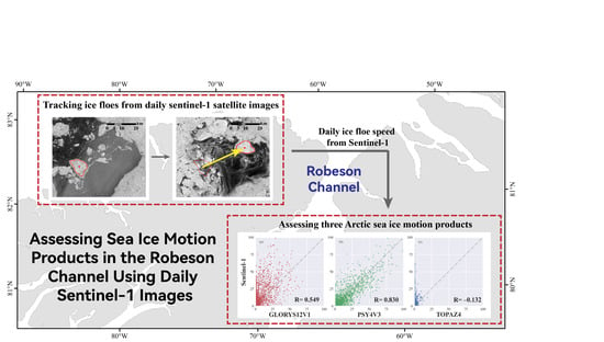
An Assessment of Sea Ice Motion Products in the Robeson Channel Using Daily Sentinel-1 Images


1
The Chinese Antarctic Center of Surveying and Mapping, Wuhan University, Wuhan 430079, China
2
Key Laboratory of Polar Surveying and Mapping, MNR, Wuhan University, Wuhan 430079, China
3
The School of Geospatial Engineering and Science, Sun Yat-Sen University, Zhuhai 519000, China
4
The Science and Technology Branch, Environment and Climate Change Canada, Government of Canada, Downsview, ON M3H 5T4, Canada
5
The Key Laboratory for Polar Science of the MNR, Polar Research Institute of China, Shanghai 200136, China
6
The School of Oceanography, Shanghai Jiao Tong University, Shanghai 200240, China
*
Author to whom correspondence should be addressed.
Remote Sens. 2022, 14(2), 329; https://doi.org/10.3390/rs14020329
Submission received: 16 November 2021
/
Revised: 1 January 2022
/
Accepted: 5 January 2022
/
Published: 11 January 2022
(This article belongs to the Special Issue Remote Sensing of Environmental Changes in Cold Regions Ⅱ)
Abstract
:Sea ice motion is an essential parameter when determining sea ice deformation, regional advection, and the outflow of ice from the Arctic Ocean. The Robeson Channel, which is located between Ellesmere Island and northwest Greenland, is a narrow but crucial channel for ice outflow. Only three Eulerian sea ice motion products derived from ocean/sea ice reanalysis are available: GLORYS12V1, PSY4V3, and TOPAZ4. In this study, we used Lagrangian ice motion in the Robeson Channel derived from Sentinel-1 images to assess GLORYS12V1, PSY4V3, and TOPAZ4. The influence of the presence of ice arches, and wind and tidal forcing on the accuracies of the reanalysis products was also investigated. The results show that the PSY4V3 product performs the best as it underestimates the motion the least, whereas TOPAZ4 grossly underestimates the motion. This is particularly true in regimes of free drift after the formation of the northern arch. In areas with slow ice motion or grounded ice floes, the GLORYS12V1 and TOPAZ4 products offer a better estimation. The spatial distribution of the deviation between the products and ice floe drift is also presented and shows a better agreement in the Robeson Channel compared to the packed ice regime north of the Robeson Channel.
1. Introduction
Sea ice motion, which is primarily driven by wind and oceanic forcing, is an essential parameter for characterizing ice advection and deformation [1,2]. The outflow of sea ice from the Arctic Ocean to the North Atlantic Ocean plays a crucial role for both the annual variation of the Arctic sea ice mass [3,4] and the formation of deep water in the North Atlantic Ocean [5]. The Arctic sea ice motion products are also important for initializing and/or verifying sea ice–ocean coupling model simulations [6].
The Robeson Channel, which is located between Ellesmere Island and northwest Greenland, is a narrow but significant gate for sea ice and freshwater outflow from the Arctic Ocean (Figure 1). This channel has contributed to the recent loss of multiyear sea ice since the majority of this type of ice in the Arctic is located north of the Robeson Channel [7,8]. The characteristics of the sea ice motion through the channel have strong intermittency and seasonal dependency [9], because of the interruption of the Arctic ice outflow during periods when an ice arch exists either at the entrance of the Robeson Channel or at the southern location of Smith Sound (the locations are shown in Figure 1). From September 2016 to August 2017, the ice influx in the Robeson Channel was blocked by the northern arch for ~110 days, while the southern arch failed to form; therefore, the ice floe is free to drift in the channel in the rest of the year. However, the phenomenon that the southern and northern arches exist simultaneously almost never happens. Essentially, the ice motion can become blocked in the channel after the development of the ice arch at Smith Sound, or accelerated after the formation of the northern arch at the entrance of the channel [10]. In addition, a few other factors affect the ice motion in the Robeson Channel. Northerly wind prevails in this region, which is conducive to the outflow of sea ice [7]. The relatively large tidal range in this area, compared with other regions in the Arctic Ocean, is another potential factor causing sea ice breakup and the enhanced oscillation of the ice motion [11]. Furthermore, the outflow of sea ice through the Nares Strait plays a crucial role in a wide range of perspectives, e.g., in the formation and cessation of the North Water Polynya in the northern Baffin Bay [12], as well as the physical and biological processes in the southern Nares Strait [13,14].
A variety of sea ice motion products are available from different sources with various spatial and temporal resolutions. These products are generally estimated from a combination of numerical simulations and observations, including buoy data and satellite observations when using data assimilation techniques (e.g., reanalysis products), or directly estimated from satellite observations, which is the case for the Ocean and Sea Ice Satellite Application Facility (OSI SAF) product and the French Research Institute for Exploitation of the Sea (IFREMER)/CERSAT product. However, only three ocean–sea ice reanalysis products are available to characterize the sea ice motion in the Robeson Channel, because of its narrow width (~30–40 km): (1) GLORYS12V1, which was derived from the Copernicus Marine Environment Monitoring Service (CMEMS) global ocean eddy-resolving reanalysis, providing sea ice motion data with a spatial resolution of 1/12° for the period of 1993–2019 [15]; (2) PSY4V3R1 (referred to as PSY4V3 here), which was derived from a global ocean analysis and prediction system implemented by CMEMS, with a horizontal resolution of 2 km near the poles for the period of 2016–2021 [16]; and (3) TOPAZ4, which was released by the Arctic—Monitoring Forecasting Centre (ARC MFC), led by the Nansen Environmental and Remote Sensing Center (NERSC), providing sea ice velocities with a spatial resolution of 35 km for the period of 1991–2019 [17]. However, uncertainties in the forcing and initial conditions of the numerical models, incomplete physical parameterization schemes, the limitation in model resolution, and uncertainties in observation data can all induce errors in the reanalysis products [18]. Therefore, these products should be assessed against observations before being applied to ice motion related studies, such as the monitoring of ice advection and ice flux, as well as before being used as the initial fields for sea ice–ocean models.
An assessment of the Arctic sea ice motion products has been conducted in a few studies, but usually either at the large scale of the Arctic Basin or in certain crucial regions, such as the Fram Strait, which is the primary gate of ice outflow to southern latitudes. Hwang and Lavergne [19] assessed the OSI SAF low- and medium-resolution products and the IFREMER/CERSAT products using in situ measurements from ice-tethered profilers. They found that the OSI SAF (medium-resolution) products have relatively low statistical errors when compared with the IFREMER product. Rozman et al. [20] compared the sea ice motion products from IFREMER, OSI SAF, and the Advanced Synthetic Aperture Radar (ASAR) instrument with in situ measurements of ice drift from moored acoustic doppler current profilers in the Laptev Sea in the winter of 2007/08. The results indicated that IFREMER has a relatively high correlation with the measurements and a low standard deviation compared to the other two products. Sumata et al. [18] investigated four coarse-resolution remotely sensed ice drift products in the Arctic Ocean, excluding narrow straits. Their results, which were derived from an intercomparison between the products and comparisons with buoy data, indicated that the differences between the products can be related to the differences in the ice conditions, including the sea ice concentration (SIC) and thickness. Ricker et al. [4] investigated the performance of sea ice motion products in the Fram Strait. Their results demonstrated clear uncertainties in the estimations of ice flux obtained using the sea ice motion products from OSI-405-c, IFREMER/CERSAT, and the National Snow and Ice Data Center (NSIDC). The accuracies of the sea ice motion products provided by NSIDC and OSI SAF have been validated using data recorded by ice drifters that were deployed in the western section of the Arctic Ocean [21]. This study concluded that the uncertainties in these products are relatively large during the ice melt season and in the marginal ice zone, compared to during the freezing season and in the pack ice zone.
However, the uncertainties of the sea ice motion products in the Robeson Channel (or any narrow channel for that matter) have not yet been assessed, partly due to a lack of direct observations of sea ice motion. Data measured by ice drifters are extremely scarce in the Robeson Channel compared with the Arctic Basin and the Fram Strait (e.g., Lei et al. [22]). To date, the intercomparison of the sea ice motion products has been a common approach, using the mean value of all the products located in the same grid [4,23,24]. However, this method is only feasible when the uncertainties of each product are well known. Moreover, remote sensing data have also been used to evaluate a few sea ice motion products [25]. Gui et al. [21] revealed that the accuracy of the sea ice motion products can be expected to be relatively low for regions close to the coast, because of shore constraints and the coarse resolution of the products. Therefore, an assessment of ice motion in narrow channels requires validation data acquired at fine spatial and temporal resolutions. Synthetic aperture radar (SAR) images can be suitable for this purpose, if daily (or more frequent) data are available. For example, Kwok et al. [26] tracked sea ice motion using the classic maximum cross-correlation (MCC) technique from sequences of SAR images acquired by the European Remote Sensing (ERS) satellites every 3 days in the Arctic Ocean and daily in the Fram Strait and Baffin Bay. The results were then used to assess the sea ice motion products derived from satellite passive microwave observations. Sumata et al. [25] assessed the errors in low-resolution sea ice motion products in the Arctic Ocean using the high-resolution sea ice motion product from the RADARSAT Geophysical Processor System (RGPS). In general, ice motion information obtained from SAR data is being increasingly used, and can be expected to have high potential for validating sea ice motion products.
The objective of this study is to assess the sea ice motion obtained from three reanalysis products in the Robeson Channel, using the drift of individual ice floes tracked from daily Sentinel-1 images covering two periods, from September 2016 to August 2017, and from January 2018 to March 2018. The influence of free versus constrained motion (i.e., linked to the presence/absence of an ice arch), regional dependence, wind speed, ice speed, as well as tidal forcing on the bias of the sea ice motion products was evaluated. The unique contribution of this study is the assessment of ice motion in a narrow channel exposed to interruption and release of ice flux due to the formation or absence of ice arches, using daily SAR data, which enabled manual Lagrangian tracking of individual ice floes. We believe that this approach of manual tracking of individual ice floes can offer the most accurate data to validate reanalysis-based or satellite-derived Eulerian sea ice motion products.
2. Materials and Methods
2.1. Study Area
The Robeson Channel, which is located between Ellesmere Island and northwest Greenland, is one of five main gates for Arctic sea ice and freshwater outflow, through which sea ice drifts southward from the Arctic Basin to Baffin Bay (Figure 1). The Robson Channel is a relatively narrow (~30–40 km), short (~80 km), and deep channel (>400 m along its axis). Local sea ice drift in the Robeson Channel is primarily driven by wind and currents. In particular, the sea ice velocity is significantly affected by meridional wind [27].
2.2. Data
2.2.1. Sea Ice Motion Products
In this study, three sea ice motion products(GLORYS12V1, PSY4V3, and TOPAZ4) were assessed. The basic information for each product is summarized in Table 1.
GLORYS12V1
The GLORYS12V1 product was generated from Version 3.1 of the Nucleus for European Modelling of the Ocean (NEMO) model, coupled with a prognostic thermodynamic-dynamic sea ice model based on Version 2 of the Louvain-la-Neuve Ice model (LIM2). The assimilated observational data include altimeter data, sea surface temperature (SST) and SIC data from satellite observations, and Coriolis Ocean dataset for Reanalysis (CORA) 4.1 temperature and salinity (T/S) data from CMEMS [15]. The atmospheric forcing for the NEMO/LIM2 model was derived from the European Centre for Medium-Range Weather Forecasts (ECMWF) reanalysis (ERA-Interim). It has been shown that the previous version of this product (GLORYS2V4) can reproduce the seasonal cycles of Arctic sea ice extent and area well [28].
This product includes three datasets and provides daily and monthly mean data for temperature, salinity, sea level, mixed layer depth, and sea ice parameters, e.g., SIC, thickness, and velocity. The daily and monthly sea ice velocity data are available from 1993 to 2019, defined on a standard regular grid of 1/12° (approximately 9 km (meridional) × 1.5 km (zonal) in our study region).
PSY4V3
The PSY4V3 product was derived from a global ocean analysis and prediction system that was implemented by CMEMS. This product was also produced by the use of a coupled ocean–sea ice model based on NEMO 3.1 and LIM2. The assimilated observational data include CORA 4.1 T/S data, Operational Sea Surface Temperature and Sea Ice Analysis (OSTIA) SST data, and OSI-450/430 SIC data. This product provides daily sea ice velocity from 2016 to 2021 on a standard regular grid, also with a resolution of 1/12°. The effectiveness of PSY4V3 in reproducing the physical variables of Arctic sea ice, e.g., the Lagrangian drift trajectory of sea ice, was assessed in Bertosio et al. [29].
TOPAZ4
The TOPAZ4 product is a subsystem released by ARC MFC that is based on an advanced sequential data assimilation method [30]. This product was produced by the use of the global Hybrid Coordinate Ocean Model (HYCOM) coupled with an elastic–viscous–plastic sea ice model. The TOPAZ4 reanalysis dataset includes both three-dimensional variables (such as current, temperature, and salinity) and two-dimensional variables (such as sea surface height, SIC, thickness, and velocity), and is ultimately interpolated onto standard grids and depths. The sea ice drift data used for the assimilation were provided by the IFREMER/CERSAT dataset for 2002–2010 [31], followed by the OSI SAF near real-time (NRT) product from 2011 onwards. Compared to buoy measurements from the basin region of the Arctic Ocean, the bias of the TOPAZ4 ice motion product shows seasonal dependence, i.e., generally overestimation in the winter months and underestimation in the summer months [32]. This dataset provides daily and monthly sea ice velocities from 1991 to 2019, with a spatial resolution of approximately 14 km (meridional) × 2.2 km (zonal) in our study region.
2.2.2. Sentinel-1 Data
Sentinel-1A and -1B are two near-polar sun-synchronous satellites developed as part of the satellite constellation of the European Space Agency’s (ESA’s) Copernicus program. The Sentinel-1A and -1B satellites were launched on 3 April 2014 and 25 April 2016, respectively. Both instruments operate at the C-band (central frequency of 5.405 GHz) with single or dual polarization. The two satellites have four operational modes: Stripmap, Interferometric Wide swath (IW), Extra-Wide swath (EW), and Wave. The EW mode products, which cover a 400 km swath at a median resolution of 20 m × 40 m, offer near-daily coverage of the Robeson Channel. In addition, the IW mode products, which cover a 250 km swath at a spatial resolution of 5 m × 20 m, have a revisit cycle of 6 days for the Robeson Channel. By combining the EW and IW modes, an approximately one-day repeat cycle can be obtained, which is suitable for monitoring the sea ice motion in the Robeson Channel. Therefore, in this study, the EW and IW mode products were chosen to track the ice floes in this region on a daily basis. Since thin ice cannot be identified in HV polarization [33], the Level-1 Ground Range Detected products of the EW and IW modes acquired in HH polarization were used in this study.
Consequently, 589 sequential Sentinel-1A and -1B images, from 1 September 2016 to 31 August 2017, and 156 sequential Sentinel-1A and -1B images, from 1 January 2018 to 21 March 2018, were used to extract the ice floe-based motion data. All images were calibrated to the backscatter coefficient in decibels and then georeferenced and resampled to 50 m × 50 m to reduce the speckle noise.
2.2.3. Wind Speed and Tide Level Data
The near-surface wind speed (10 m) data used in the assessment were obtained from ERA5 [34], which is the successor to ERA-Interim. The data were generated by combining simulated data and observations at a spatial resolution of 0.25° × 0.25° (4.3 km (meridional) × 27.8 km (zonal) for the study area). The higher accuracy of ERA5 for the wind speed has been proven via comparisons with other reanalysis data from the US National Centers for Environmental Prediction/National Center for Atmospheric Research (NCEP/NCAR), the NCEP/Department of Energy (NCEP/DOE) reanalysis, and ERA-Interim in the region of the Robeson Channel [10].
Tidal forcing can regulate the magnitude of sea ice velocity by strengthening the semidiurnal oscillation and promoting the fragmentation of large floes, which, in turn, can be expected to affect the accuracy of sea ice motion products. In this study, the influence of year-round tidal forcing on the accuracy of the sea ice motion products was evaluated using data obtained from tidal gauge measurements, taken between 1 September 2016 and 31 August 2017, at the Wrangel Bay tide station (Figure 1) in the Robeson Channel [35]. Qualitatively, the daily tidal range was used to assess the influence of tidal forcing on the accuracy of the sea ice motion products.
2.3. Methods
2.3.1. Estimation of Sea Ice Motion Using Sentinel-1A/-1B Images
As mentioned before, generating ice floe motion using the widely applied MCC technique is not applicable in narrow water passages. Accordingly, we estimated the velocity of individual ice floes during their lifetime within the Robeson Channel. This was performed by tracking selected ice floes in the daily Sentinel-1A/-1B images. A detailed procedure of ice floe tracking method is presented in [10].
In this study, two datasets of Sentinel-1A/-1B images were used to estimate the daily ice floe drift. The first dataset covered a period of one year from 1 September 2016 to 31 August 2017 with 589 Sentinel-1A/-1B images. In this dataset, 129 ice floes were tracked. A total of 1830 samples of ice floe locations were obtained from this dataset, from which the sea ice velocity vectors were estimated, with most being obtained in October and November of 2016 (Table 2). Since the northern ice arch formed on 25 January 2017, the ice floe stopped moving in the Robeson Channel until 11 May 2017. Therefore, the second dataset was used to study ice floe motion covering the period of January to March 2018. In this dataset, 156 Sentinel-1A/-1B images were used, 85 ice floes were tracked, and a total of 582 samples of ice floe locations were obtained. The southern ice arch existed between 28 February and 1 July 2018.
2.3.2. Grouping of the Ice Motion Data
For the purpose of assessing the reanalysis products of sea ice motion, the ice floe speed data obtained from the daily Sentinel-1 images were grouped into three groups: (1) ice motion in the Robeson Channel in the absence of an ice arch; (2) ice motion in the Robeson Channel in the presence of the northern arch; and (3) ice motion in the Robeson Channel in the presence of the southern arch. In the absence of an ice arch, the channel usually features a high SIC, with thick floes as the ice influxes from the Lincoln Sea. This results in a relatively slow ice motion, except for the ice floes that are surrounded by open water. The data in this group were available for the periods of September–December in 2016, June–August in 2017, and 1 January to 21 February in 2018. When the northern ice arch was formed on 25 January 2017 and until it collapsed on 11 May 2017, the ice influx was blocked. This resulted in the formation of a polynya-like ice field with fewer ice floes (mostly thin), leading to a nearly free drift regime. Under this condition, the impacts of the wind and oceanic forcing on the ice motion were enhanced, resulting in faster ice motion [10,36]. After the formation of the southern arch between 22 February and 1 July 2018, the ice slowed down in the channel until it eventually came to a stop.
2.3.3. Assessment of the Sea Ice Motion Products
The gridded ice motion from the three reanalysis products was generated for 12:00 UTC. To match this, we should emphasize again that the ice floe speed from Sentinel-1 was calculated at the same time, by assuming that the ice floe drift was linear between the two satellite revisit times. The calculated ice floe drift along the trajectory (magnitude and direction) was then compared to the product’s drift at the nearest grid point. Since the time span of the two successive Sentinel-1 images used to calculate the ice floe motion was not a fixed value (~24 h), due to the deviation of the satellite revisit time, the orientation of the ice floe drift was not taken into account when evaluating the ice motion speed from the reanalysis products.
In this study, the correlation coefficient (R), mean absolute error (MAE), root-mean-square error (RMSE), and skewness were used to quantify the differences in the magnitudes between the ice drift from each of the examined sea ice motion products and that from Sentinel-1. In addition, histograms of the ice motion, kernel density estimation, and box plots were also provided. Two parameters (the bin width and the end points of the bins) need to be considered in the construction of a histogram. Kernel density estimation, as one of the most commonly used non-parametric estimation methods, can provide useful information about the features in a dataset without the uncertainty of the bin widths and end points [37]. A box plot, which is a way of characterizing a dataset based on an interval scale, can represent the shape of a distribution, and the maximum, minimum, and upper and lower quartiles in a dataset.
3. Results
3.1. Daily Ice Floe Speed
Figure 2 presents the daily ice floe speed obtained using the sequential Sentinel-1 images, as well as the wind speed. Each red point represents the daily average ice drift from all the identifiable ice floes inside the Robeson Channel. Each green point represents the daily average wind speed from ERA5 for the four grid points closest to the ice floe. The blue areas in the figure mark the periods of presence of the northern or southern ice arch.
Figure 2 shows that the daily average ice floe speed fluctuates significantly within a short period (and even between successive days). However, it should be kept in mind that not all the ice floes in the channel on any given day were tracked and used to calculate the motion in the sequential daily Sentinel-1 images. This can partly explain the fluctuations. However, the main cause is likely the combined actions of the wind and current forcing, given their possible different directions, as well as the interaction between ice floes, which varies according to the variable SIC surrounding the ice floes. In addition, some ice floes used in the calculation may have been slowed down as a result of friction with the coastline or fast ice. Fluctuations of ice floe speed can still be observed during the periods of the northern and southern ice arches.
Figure 2a shows the data from September 2016 to August 2017, covering the period of the northern arch, and Figure 2b shows the data from January to March 2018, covering the period of the southern arch. During the period of the northern ice arch (the blue area in Figure 2a), the SIC in the Robeson Channel can be expected to be low, with thin ice dominating. The average ice floe speed during this period was 30.77 km/d, which is slightly higher than the average speed of 26.98 km/d observed outside this period. This is a confirmation of the enhanced ice motion in ice cover with a lower SIC and ice floe thickness. During the period of the southern ice arch (the blue area in Figure 2b), the ice floe speed continued to decelerate as the ice continued to accumulate in the channel, until the ice drift came to a complete stop on 21 March 2018.
Figure 2 also shows that the ice floe speed is correlated with the wind speed peak-to-peak daily variability, in most cases. Before the formation of the northern ice arch, the correlation between the ice floe speed and wind speed was 0.782 at a confidence level of 0.01. This increased to 0.827 during the period of the northern arch. After the collapse of the northern arch on 11 May 2017, the ice flux from the Lincoln Sea resumed, which enhanced the interactions between the ice floes and reduced the correlation to 0.706.
Some ice floe speed anomalies (>75 km/d) are also apparent in Figure 2. On 13 and 18 December 2016, the ice floe speed reached 89.99 km/d and 81.78 km/d, respectively. These anomalies occurred because several ice floes were located at the entrance of or in Hall Basin (Figure 1), which is a relatively open water area compared with the overall ice floe situation in the Robeson Channel. Moreover, a strong southerly wind of 19.79 km/h prevailed during that period (Figure 3). The highest ice floe speed of 99.1 km/d was observed between 21 and 22 February 2017, during the period of the northern ice arch formation. This was triggered by strong southerly wind gusting to 49.90 km/h. The ratio of the ice floe to wind speed in this case was 0.083.
After the collapse of the northern ice arch on 11 May 2017, a large fast ice area attached to the coast of Greenland north of the Robeson Channel (marked by the reddish area in Figure 4) broke off and induced ice floes that drifted at an anomalous speed of >75 km/d. Breakoff occurred twice on 23 and 31 May 2017, and was instigated by a steady and gradually enhanced wind of 9.49 km/h (mean value) blowing parallel to the axis of the channel (Figure 5). The underlying point from this information is the variability of the ice floe motion, which cannot be captured by the gridded model results. Therefore, while model results can be useful for the calculation of ice flux and other climatological parameters, they should be considered with caution when it comes to marine operation applications.
In the open sea, ice typically drifts at a speed of approximately 2% of the wind speed and about 25° to the right of the wind in the Northern Hemisphere [38]. However, the ice floe speed data from the present dataset shows that this ratio is significantly larger, as it fluctuates between 0 and 60%. In general, the wind has more of an effect on ice drift in narrow channels than in the open sea, particularly when the wind direction coincides with the constrained geographic orientation of the channel. The cohesion of the ice cover is also an important factor when studying the influence of the direction and magnitude of the wind on the movement of ice floes. The cohesion of the ice cover related to ice thickness and concentration; it is relatively low in this study since only individual floes with the relatively low surrounding sea ice concentration and abundant leads or open water were tracked. In addition, the sea ice movement would be affected by current stress, horizontal gradient (sloping sea surface) stress, Coriolis stress, and ice internal stress. In the strait regions, even if the sea ice concentration is low, the ice internal stress can be ignored, and the current stress still can play a strong role due to the gorge effect (e.g., [22,39]). In the study region, the role of the current, especially tidal current [11], cannot be ignored. Therefore, although the ice floes are mainly related to wind force, it can also be affected by other factors, especially current stress. During the time with relative weak wind forcing, the contribution of current stress would be enhanced. The air temperature would play trivial roles on the ice motion through regulating the consolidation of sea ice, and the water temperature is not a factor that affect motion because the water covered by the ice would have a small temperature variation.
3.2. Overall Assessment
For an overall assessment of the three sea ice motion products, the data were compared to the Sentinel-1 ice floe speed from the entire datasets for 2016/2017 and 2018. Figure 6 presents scatter plots of the ice floe drift versus the gridded ice motion from each reanalysis product. The frequency distributions of the ice speed derived from the three sea ice motion products, as well as Sentinel-1, are also shown.
The scatter plot obtained using the GLORYS12V1 data shows that this product underestimates the ice drift speed, and most of the speeds from this reanalysis product do not exceed 27 km/d. Uotila et al. [28] also indicated an underestimation of the freshwater exports through the Fram Strait, Barents Sea, Davis Strait, and Bering Strait using the GLORYS2V4 product. The R value from the GLORYS12V1 product is moderate (0.549), compared with the ice floe speed obtained using the Sentinel-1 images, but still significant at a statistical level of 0.01. The scatter plot and the distribution of the PSY4V3 product present the best agreement with the ice floe speed obtained using the Sentinel-1 images. Moreover, a relatively high correlation between the two datasets is shown, with an R value of 0.830 (p < 0.001). Conversely, the TOPAZ4 product performs poorly as it gives extremely low motion values (<5 km/d), with a very low R value of −0.132, and is insignificant at a statistical confidence level of 0.05. This product is a near-complete mismatch with the results derived from the Sentinel-1 imagers. According to Simonsen et al. [17], the TOPAZ4 product assimilates ice drift data from OSI-405-c. This dataset covers most of the central Arctic Ocean, but often has a data gap in the region of the Robeson Channel.
The kernel density and the three parameters (MAE, RMSE, and Skewness) representing the deviation of the sea ice motion product from the ice floe drift are presented in Figure 7. Among the three products, PSY4V3 has the lowest MAE and RMSE when compared to the ice floe speed obtained from the Sentinel-1 images, with values of 6.35 km/d and 9.67 km/d, respectively. The probability distribution of the deviation of the PSY4V3 product from the estimated ice floe drift peaks near 0 km/d, with a lowest absolute skewness of −0.27, suggesting a near-normal distribution. The negative skewness from the data of the three products indicates that the ice motion is generally underestimated by these products, especially the TOPAZ4 product. As a result of the deviation between the ice motion data derived from the TOPAZ4 product and that from Sentinel-1 is quite large, the data from the TOPAZ4 product were not used in the assessments described below. The TOPAZ4 product is not deemed suitable for depicting the sea ice motion in the region of the Robeson Channel.
The above assessment was conducted without considering the ice motion direction in relation to the wind direction. In the rest of this Section, we discuss the difference between the direction of the ice floe drift obtained from Sentinel-1 and that from the GLORYS12V1 and PSY4V3 products. This is represented using rose diagrams in Figure 8a–c for the data north of the Robeson Channel, and in Figure 8d–f for the data inside the Robeson Channel. The length of each spoke around the circle in the diagram indicates the amount of time that the ice floe drifts in a particular direction. The colors of the spokes indicate the categories of wind speed.
From Figure 8a–c, it can be seen that the dominant orientation of the ice floe motion is from south-southeast (SSE) to south or southwest (SW). However, ice drift heading north is observed in the ice floe drift data from Sentinel-1. This is the only difference between the ice motion reanalysis data (GLORYS12V1 and PSY4V3) and the ice floe drift data from Sentinel-1. The PSY4V3 product is slightly superior to the GLORYS12V1 product. In the orientation from SSE to SW, the ice floes from Sentinel-1 and PSY4V3 have similar motion speeds and orientation distributions, whereas GLORYS12V1 clearly underestimates the speed. As for the situation inside the Robeson Channel, due to the limitation of the coastal landform, the ice floe motion is concentrated to the SW and south-southwest (SSW). Similar to the area north of the Robeson Channel, the GLORYS12V1 and PSY4V3 products are unable to simulate the northward ice motion.
4. Discussion
4.1. Impact of the Ice Arches on the Bias of the Sea Ice Motion Products
As mentioned in Section 2.3.2, the presence or absence of an ice arch impacts the ice types and SIC in the Robeson Channel. The presence of the northern ice arch causes more free ice drift, whereas the southern arch causes the congestion of the channel with thick ice, and eventually leads to stagnation. Figure 9 shows scatter plots of the Sentinel-1 ice floe speed versus the sea ice motion product for three situations of ice in the Robeson Channel: (1) without an ice arch; (2) in the presence of the northern arch; and (3) in the presence of the southern arch. Table 3 lists the correlation coefficient (R) values of the data under the aforementioned conditions.
Under the no arch condition, R is 0.826 and 0.524 for PSY4V3 and GLORYS12V1, respectively. This is not significantly different from the values resulting from the use of the entire dataset. Under the presence of the northern arch, where the surface is covered with sparse and thin ice floes, the R value for GLORYS12V1 increases slightly to 0.563 and decreases slightly to 0.786 for PSY4V3. These are marginal changes, so we do not consider that the behavior of the two products is affected by the presence of the northern arch. When the southern arch forms, the R value decreases remarkably to 0.544 for PSY4V3 and remains at nearly the same value (0.554) for the GLORYS12V1 product. The formation of the southern arch causes the jamming of the ice floes in the channel. The lower R value for the PSY4V3 product means that the product fails to account for the interactions between the floes in a compacted ice regime. On the other hand, the tendency of the GLORYS12V1 product to underestimate the motion makes it insensitive to the motion of a jammed ice field. The results listed in Table 3 show the superiority of the PSY4V3 product over the GLORYS12V1 product under both the conditions of the presence and absence of the northern arch, with no difference between the behavior of either product under the presence of the southern arch. It is worth noting that a period of no ice motion was encountered between 21 March 2018 and 1 July 2018, shortly after the formation of the southern ice arch. During this period, GLORYS12V1 produced an average motion speed of 0.06 km/d, while PSY4V3 produced an average motion of 15.64 km/d. Once again, this does not mean that the GLORYS12V1 product is better overall, but rather that it produces better results in situations of slow or no ice motion. In fact, the TOPAZ4 product reproduces the correct zero motion during the period of stagnation, although it is not reliable when the ice floe starts to drift.
4.2. Influence of the Wind Speed on the Accuracy of the Sea Ice Motion Products
Wind is an important factor affecting ice drift, with an increasing influence in regions with a low SIC and thin ice [10]. In this section, the influence of wind on the accuracies of the sea ice motion products is evaluated. The wind speed is grouped into two categories separated by the median value of 9.86 km/h. The accuracies of each product compared to the ice floe speed from Sentinel-1 are then compared for each wind category in Table 4.
All of the statistics listed in Table 4 indicate that the PSY4V3 product performs better than the GLORYS12V1 product under the different wind speed regimes. The atmospheric forcing used in the PSY4V3 product is taken from the ECMWF Integrated Forecast System [40], while the forcing in the GLORYS12V1 product is taken from the ERA-Interim Reanalysis in earlier years and the ERA5 Reanalysis in recent years. The relatively high uncertainty of ERA-Interim for the wind fields compared to ERA5 has been demonstrated by Shokr et al. [10]. Assimilating the data of ERA-Interim in the early stage is a potential error source for the GLORYS12V1 product.
Note that the accuracies of the sea ice motion products are slightly better (especially for the GLORYS12V1 product) in the low-speed wind range than in the high-speed range. This is likely because stronger wind forcing can enhance the interactions between the ice floes and weaken the ice motion response to wind forcing [41]. This mechanism is primarily related to high-frequency processes, which are likely to be ignored in the numerical models (e.g., Heil and Hibler [42]). However, the influence of the different wind regimes on the accuracy of the products is moderate because the differences in the accuracies under the two wind regimes are much lower than the accuracies themselves, especially for the PSY4V3 product. For example, the difference in the RMSE values of PSY4V3 corresponding to the two wind regimes is 0.15 km/d (or −4.50%).
4.3. Influence of Ice Floe Speed on the Deviation of the Sea Ice Motion Products
Does the sea ice speed itself influence the accuracy of the PSY4V3 and GLORYS12V1 products? Sumata et al. [25] indicated that the uncertainty of several sea ice motion products versus the estimation from RGPS observations in the Arctic Ocean depends on the sea ice speed. To further explore the influence of ice floe speed on the deviation in the sea ice motion products, the speed was grouped into 10 bins ranging from 0 to 100 km/d, as shown in Figure 10.
The deviation of the PSY4V3 and GLORYS12V1 products from the ice floe speed (measured in terms of the MAE) is negligible when the ice floe drift does not exceed 10 km/d. The MAE then increases with the increasing ice floe speed. A significant positive relationship (R2 = 0.984, p < 0.001) between the GLORYS12V1 MAE and the ice floe speed can be identified in Figure 10. When the ice floe speed is between 90 km/d and 100 km/d, the GLORYS12V1 MAE is ~73 km/d, which is approximately 15 times larger than the value when the ice floe speed is less than 10 km/d. Conversely, the MAE from the PSY4V3 data is relatively stable when the ice floe speed is greater than 30 km/d. However, the PSY4V3 MAE shows fluctuations when the ice floe speed is between 70 and 100 km/d. This can be partly attributed to the limited samples of ice floe speed records from the Sentinel-1 images, with only 3 and 11 tracked ice floes having ice speeds of 90–100 km/d and 80–90 km/d, respectively. In general, the influence of the ice floe speed on the accuracies of the products is smaller for PSY4V3 than for GLORYS12V1. As previously mentioned, the data used in the assimilation of the GLORYS12V1 product are mainly obtained from reanalysis data, which differ from the satellite image-based ice speed results. Conversely, the PSY4V3 product partly assimilates satellite data (Special Sensor Microwave Imager Sounder (SSMIS) data in recent years), which are more similar to the satellite image-based estimated ice speed.
4.4. Influence of Tidal Forcing on the Bias of the Sea Ice Motion Products
The Nares Strait (including the Robeson Channel) has a relatively large tidal range compared with other regions in the Arctic Ocean. Davis et al. [11] indicated that the strongest M2 and S2 tides occur in the Kane Basin and to the south. Whether the accuracies of the reanalysis products are influenced by the tides in the Robeson Channel is unknown. Therefore, this study combined the analysis of the deviation of the PSY4V3 and GLORYS12V1 products with that of the tidal range data to investigate the influence of year-round tidal forcing on these products.
A significant correlation between the tidal range and the ice floe speed from the Sentinel-1 images is apparent, only in certain months (Figure 11). For example, the negative R value (−0.771, p < 0.01) in February 2017 indicates that the ice motion was greatly influenced by the strong tidal effect for some ice floes. Around 12 February, the large tidal range induced a low ice floe speed. Davis et al. [11] observed strong tides in the Nares Strait resulting from a standing wave with a semidiurnal tide cycle. Therefore, the horizontal motion of an ice floe can be slowed under the forcing of a standing wave. However, the monthly correlation is not stable, and the correlation is insignificant for 7 months at the statistical level of 0.05.
Furthermore, the relationship between the tidal range and the deviation between the sea ice motion products and the ice drift data is insignificant for most months (Figure 12). This is because the tidal frequency in the Robeson Channel is twice per day (M2 tide). Therefore, it cannot be captured in the daily data from the Sentinel-1 images. Accordingly, further studies need to be conducted using satellite images with a higher temporal resolution.
4.5. Spatial Differences in the Accuracy of the Sea Ice Motion Products
As the SIC regulates the interactions between ice floes, it constitutes another factor affecting ice drift [43], and consequently influences the accuracy of the remote sensing based products for sea ice motion [21]. The SIC is different for regions inside and outside the Robeson Channel, with higher values outside (Figure 13). Therefore, we assessed the performance of each product separately in the two sub-regions.
Violin plots, which combine a box plot and kernel density, are used to represent the probability distributions of the deviation between the sea ice motion products and the ice floe speed obtained from the Sentinel-1 images in Figure 14. Outside the Robeson Channel, the probability distributions of the deviation of the PSY4V3 and GLORYS12V1 products versus the ice floe speed estimated using the Sentinel-1 images are similar, with a single steep peak and a normal distribution. However, the peak of the GLORYS12V1 product is slightly lower than 0 km/d, which indicates that the ice motion is slightly underestimated by the GLORYS12V1 product in this sub-region.
Inside the Robeson Channel, the distributions of the deviation of the PSY4V3 and GLORYS12V1 products also approximate a normal distribution. However, they have a larger standard deviation and a broader peak compared to the distributions found outside the Robeson Channel. The data from GLORYS12V1 also peak at a value that is lower than 0 km/d, and the probability distribution reveals an asymmetric pattern, with the absolute value of the upper quartile being lower than that of the lower quartile. Both statistical patterns indicate that the ice motion is underestimated by the GLORYS12V1 product inside the Robeson Channel, which is generally consistent with the distribution of the kernel density shown in Figure 7a. Table 5 includes a few statistical parameters to summarize the accuracy of each product inside and outside the Robeson Channel. The different SICs between the outer and inner sub-regions result in different mean ice speeds of 7.00 km/d and 28.99 km/d, respectively. To remove the influence of the ice speed itself, the ratios of both MAE and RMSE to the mean speed were calculated. The ratio of MAE to mean speed is called the relative deviation. The PSY4V3 product has lower MAE, RMSE, and relative deviation values than GLORYS12V1 for both sub-regions, which suggests that the PSY4V3 product provides a more accurate representation of the sea ice motion for both regions.
The ratios of the MAE/mean speed and RMSE/mean speed present opposite characteristics, when compared to the MAE and RMSE values. That is to say, both ratios are smaller inside than outside the Robeson Channel for both products. Therefore, the differences in the MAE and RMSE values for the two sub-regions are primarily caused by the differences in ice speed, which are in turn related to the differences in the SIC. Outside the Robeson Channel, the ice motion pattern is not free drift, but is impacted by the internal stress, to a high degree, which is not easy to accurately capture in the reanalysis products. This likely leads to greater relative MAE and RMSE values, compared with the sub-region inside the channel.
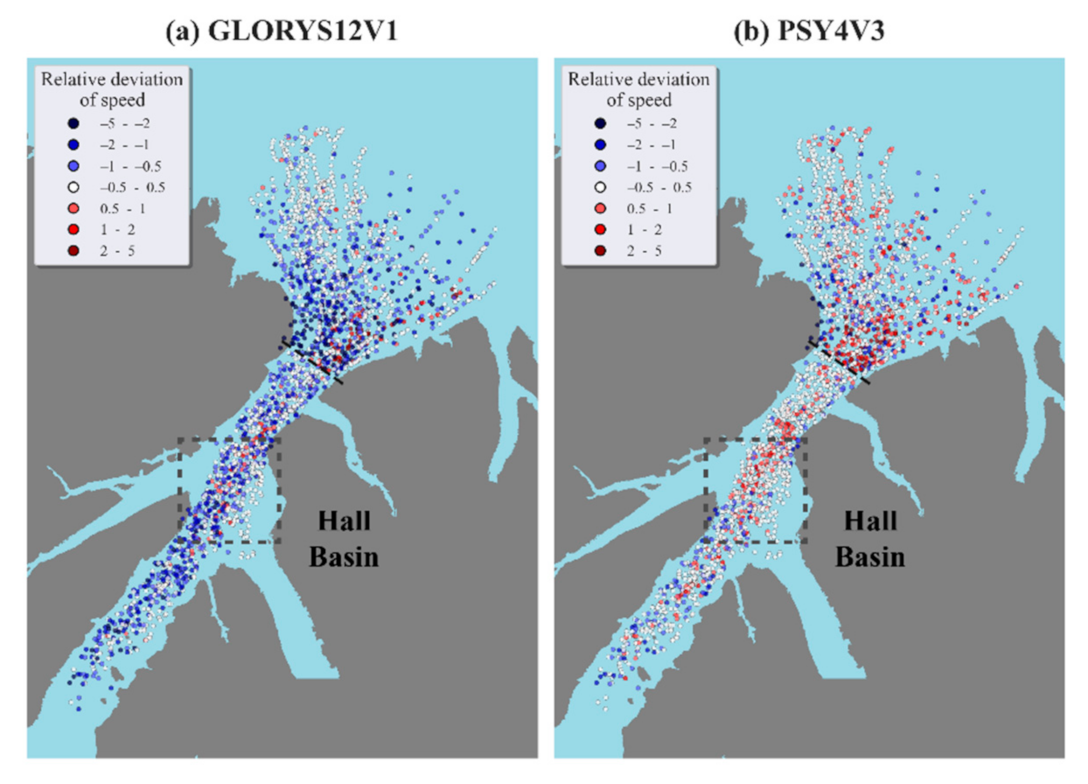
Figure 15 presents the spatial distribution of the relative deviation of each product, compared with the ice floe speed from the Sentinel-1 images. Outside the Robeson Channel, and especially in the region near the entrance from the Lincoln Sea to the Robeson Channel, the negative deviations are larger than the positive relative deviations (Figure 15a), which also indicates that the ice motion is generally underestimated by the GLORYS12V1 product in this sub-region. Conversely, the positive and negative relative deviations are comparable in the sub-region outside the channel for the PSY4V3 product (Figure 15b), which agrees with the near-normal probability distribution of the deviation (Figure 14). Note that the relative deviation of the PSY4V3 product is also relatively large near the entrance, which can be due to the instability of the SIC in this sub-region.
Inside the Robeson Channel, it is clear that the PSY4V3 product performs better than the GLORYS12V1 product, with a smaller relative deviation error. However, the distributions of the relative deviation are different for the two products. The GLORYS12V1 product performs worse in the region south of Hall Basin, while the PSY4V3 product performs worse within Hall Basin. This can be due to regional differences in the atmospheric forcing or currents, which is difficult to assess quantitatively. More specifically, the relative deviation of the speed is between −0.5 and 0.5 for the PSY4V3 product (in Figure 15b) near the gate inside the Robeson Channel, which indicates that the ice motion is accurately simulated at this gate by the PSY4V3 product. Therefore, PSY4V3 has great potential to be used to estimate the ice flux through the Robeson Channel.
5. Conclusions
In this study, we validated the ice motion data from the three ocean–sea ice reanalysis products of PSY4V3, GLORYS12V1, and TOPAZ4 in the Robeson Channel. This is a narrow but significant channel for sea ice and freshwater outflow from the Arctic Ocean. The reanalysis ice motion product within this channel is available only from the three aforementioned products. Ice floe speeds (magnitude and direction) were extracted from daily Sentinel-1 images between September 2016 and March 2018, including periods of ice arch formation at the northern entrance of the channel and the northern location of Smith Sound. These satellite-derived ice floe drift data (Lagrangian representation) were used to validate the gridded reanalysis products (Eulerian representation).
The daily average ice floe speed showed a significant fluctuation (Figure 2), which was probably caused by the complex integrated influence of wind, current forcing, and the floe track being surrounded by different ice concentrations or being close to fast ice edges. Anomalies of ice floe speed (e.g., >75 km/d) were also apparent in the data, which were mainly triggered by the prevailing strong northerly wind in areas of free drift.
The validation of the ice motion reanalysis products showed general underestimation by the three products with respect to the ice floe speed from Sentinel-1 images (Figure 6). The PSY4V3 product showed the least underestimation, with the lowest MAE of 6.35 km/d and RMSE of 9.67 km/d. It also showed the best correlation with the ice floe speed from Sentinel-1 images (R = 0.830, p < 0.001). TOPAZ4 grossly underestimated the ice motion, and it should only be used in areas where the ice motion is negligible. This was likely due to the lack of sea ice data in the process of assimilation of the observations. For this reason, in this study, focus was placed on the evaluation of the PSY4V3 and GLORYS12V1 products.
The ice motion from these two products was evaluated under three situations of ice drift in the Robeson Channel: (1) in the absence of an ice arch; (2) in the presence of the northern arch, where the condition of free drift is more likely; and (3) in the presence of the southern arch, where the condition of compacted ice is likely. While the PSY4V3 product still produced better results in both conditions in terms of deviation and correlation with the ice floe drift data (Figure 9; Table 3), no difference was found between the behaviors of either product in the presence or absence of the northern arch. In contrast, under the condition of the southern arch, the correlation between the PSY4V3 product and the ice floe speed decreased from 0.830 to 0.544, indicating the sensitivity of this product to ice concentration. No similar decrease was found for the GLORYS12V1 product, which provides superior results but only in situations of slow or no ice drift (i.e., compacted ice).
The impacts of the absolute magnitude of the wind and ice floe speed, and that of tidal forcing, on the accuracies of the sea ice motion products were also explored. The impact of wind was found to be moderate, as the differences in the accuracies of each reanalysis product under two wind regimes are much lower than the accuracies themselves, especially for the PSY4V3 product (Table 4). The deviation of the two reanalysis products compared with the ice floe speed was negligible when the ice floe speed was lower than 10 km/d (Figure 10). The deviation then increased linearly at a high rate after 10 km/d for the GLORYS12V1 product and at much less rate for the PSY4V3 product. The impact of tidal forcing on the daily sea ice motion products was not as significant as its influence on the ice floe speed itself, which was primarily related to the relatively coarse temporal resolution of the reanalysis products and the ice floe speed from the Sentinel-1 images (Figure 12).
Furthermore, a spatial difference in the accuracies of the sea ice motion products was identified. The relative deviation from the ice floe speed inside the channel was better than that obtained outside the channel (Figure 14; Table 5). This was essentially related to the differences in the SIC, which is higher outside the channel. The spatial differences in the accuracy of the PSY4V3 product were smaller than those of the GLORYS12V1 product for both sub-regions. Moreover, the PSY4V3 product presented a high performance near the gate to the Robeson Channel (Figure 15), which reveals its high potential for quantifying the ice flux through the Robeson Channel.
Overall, the PSY4V3 product presented better effectiveness, robustness, and accuracy in the Robeson Channel compared to the other two products, and has better potential for characterizing the ice motion and estimating sea ice or freshwater outflow flux through the channel. The quantitative results of this study will provide useful information when choosing products to monitor variations in the ice motion or sea ice flux at various temporal scales in the Robeson Channel or similar narrow channels. Johnson et al. [44] indicated that the assimilation of the sea ice motion can lead to an improvement in the simulation of sea ice thickness in the Arctic Ocean. Therefore, the results of this study can also provide background information when choosing products to simulate sea ice thickness. Furthermore, this study proved the applicability that the ice floe speed from sequential daily Sentinel-1 images can be considered as virtual Lagrangian buoy data, and can be used in a wide variety of studies of sea ice dynamics. However, such data cannot represent all the ice floes drifting in the channel, due to the limitation of manual identification of ice floes from Sentinel-1 images, which are seriously affected by noise.
Author Contributions
T.L. conceived and designed the study, conducted data analyses, and drafted the manuscript. Z.W. collected and analyses data. M.S. participated in the design of some experiments and manuscript writing. R.L. participated in the design of some experiments and revised the paper. Z.Z. participated in the manuscript writing and review. All authors have read and agreed to the published version of the manuscript.
Funding
This work was supported in part by the National Key Research and Development Program of China under Grant 2021YFC2803301 and Grant 2018YFC1406102, in part by the National Natural Science Foundation of China under Grant 41976219 and Grant 41861134040, and in part by the Key Laboratory for Polar Science of the MNR under Grant KP202004.
Institutional Review Board Statement
Not applicable.
Informed Consent Statement
Not applicable.
Data Availability Statement
Sentinel-1A/-1B product (https://scihub.copernicus.eu/, accessed on 5 February 2021); the ERA5 reanalysis products (https://cds.climate.copernicus.eu/cdsapp#!/dataset/reanalysis-era5-single-levels?tab=overview, accessed on 5 February 2021); GLORYS12V1, PSY4V3, and TOPAZ4 products (https://resources.marine.copernicus.eu/?option=com_csw&task=results, accessed on 5 February 2021); and tide data (https://mobilegeographics.com, accessed on 20 November 2020).
Conflicts of Interest
The authors declare no conflict of interest.
References
- Zhang, J.; Woodgate, R.; Moritz, R. Sea ice response to atmospheric and oceanic forcing in the Bering Sea. J. Phys. Oceanogr. 2010, 40, 1729–1747. [Google Scholar] [CrossRef]
- Spreen, G.; Kwok, R.; Menemenlis, D. Trends in Arctic sea ice drift and role of wind forcing: 1992–2009. Geophys. Res. Lett. 2011, 38, L19501. [Google Scholar] [CrossRef] [Green Version]
- Kwok, R. Outflow of Arctic Ocean sea ice into the Greenland and Barents Seas: 1979–2007. J. Clim. 2009, 22, 2438–2457. [Google Scholar] [CrossRef] [Green Version]
- Ricker, R.; Girard-Ardhuin, F.; Krumpen, T.; Lique, C. Satellite-derived sea ice export and its impact on Arctic ice mass balance. Cryosphere 2018, 12, 3017–3032. [Google Scholar] [CrossRef] [Green Version]
- Ionita, M.; Scholz, P.; Lohmann, G.; Dima, M.; Prange, M. Linkages between atmospheric blocking, sea ice export through Fram Strait and the Atlantic Meridional Overturning Circulation. Sci. Rep. UK 2016, 6, 32881. [Google Scholar] [CrossRef] [PubMed] [Green Version]
- Martin, T.; Gerdes, R. Sea ice drift variability in Arctic Ocean Model Intercomparison Project models and observations. J. Geophys. Res. Oceans 2007, 112, C04S10. [Google Scholar] [CrossRef] [Green Version]
- Kwok, R.; Toudal Pedersen, L.; Gudmandsen, P.; Pang, S.S. Large sea ice outflow into the Nares Strait in 2007. Geophys. Res. Lett. 2010, 37, L03502. [Google Scholar] [CrossRef] [Green Version]
- Moore, G.W.K.; Howell, S.E.L.; Brady, M.; Xu, X.; McNeil, K. Anomalous collapses of Nares Strait ice arches leads to enhanced export of Arctic sea ice. Nat. Commun. 2021, 12, 1. [Google Scholar] [CrossRef]
- Kwok, R. Variability of Nares Strait ice flux. Geophys. Res. Lett. 2005, 32, L24502. [Google Scholar] [CrossRef] [Green Version]
- Shokr, M.E.; Wang, Z.; Liu, T. Sea ice drift and arch evolution in the Robeson Channel using the daily coverage of Sentinel-1 SAR data for the 2016–2017 freezing season. Cryosphere 2020, 14, 3611–3627. [Google Scholar] [CrossRef]
- Davis, P.E.D.; Johnson, H.L.; Melling, H. Propagation and vertical structure of the tidal flow in Nares Strait. J. Geophys. Res. Oceans 2019, 124, 281–301. [Google Scholar] [CrossRef] [Green Version]
- Dumont, D.; Gratton, Y.; Arbetter, T. Modeling the dynamics of the North Water polynya ice bridge. J. Phys. Oceanogr. 2009, 39, 1448–1461. [Google Scholar] [CrossRef]
- Barber, D.; Marsden, R.; Minnett, P.; Ingram, G.; Fortier, L. Physical processes within the North Water (NOW) polynya. Atmos. Ocean 2001, 39, 163–166. [Google Scholar] [CrossRef]
- Tremblay, J.É.; Gratton, Y.; Carmack, E.C.; Payne, C.D.; Price, N.M. Impact of the large-scale Arctic circulation and the North Water Polynya on nutrient inventories in Baffin Bay. J. Geophys. Res. Oceans 2002, 107, C8. [Google Scholar] [CrossRef]
- Fernandez, E.; Lellouche, J.M. Product user manual for the Global Ocean Physical Reanalysis Product GLORYS12V1. Copernic. Prod. User Man. 2018, 4, 1–15. [Google Scholar]
- Lellouche, J.M.; Greiner, E.; Galloudec, O.L.; Garric, G.; Regnier, C.; Drevillon, M.; Benkiran, M.; Testut, C.E.; Bourdalle-Badie, R.; Gasparin, F.; et al. Recent updates to the Copernicus Marine Service global ocean monitoring and forecasting real-time 1∕12° high-resolution system. Ocean Sci. 2018, 14, 1093–1126. [Google Scholar] [CrossRef] [Green Version]
- Simonsen, M.; Hackett, B.; Bertino, L.; Røed, L.R.; Waagbø, G.A.; Drivdal, M.; Sutherland, G. Product User Manual for Arctic Ocean Physical and Bio Analysis and Forecasting Products: ARCTIC_ANALYSIS_FORECAST_PHYS_002_001_a, ARCTIC_ANALYSIS_FORECAST_BIO_002_004 and Physical and Bio Reanalysis Products: ARCTIC_REANALYSIS_PHYS_002_003, ARCTIC_REANALYSIS_BIO_002_005; CMEMS: Toulouse, France, 2019. [Google Scholar]
- Sumata, H.; Lavergne, T.; Girard-Ardhuin, F.; Kimura, N.; Tschudi, M.A.; Kauker, F.; Karcher, M.; Gerdes, R. An intercomparison of Arctic ice drift products to deduce uncertainty estimates. J. Geophys. Res. Oceans 2014, 19, 887–4921. [Google Scholar] [CrossRef] [Green Version]
- Hwang, B.; Lavergne, T. Validation and Comparison of OSI SAF Low and Medium Resolution and IFREMER/Cersat Sea Ice Drift Products; CDOP-SG06-VS02; The EUMETSAT Network of Satellite Application Facilities: Darmstadt, Germany, 2010. [Google Scholar]
- Rozman, P.; Hölemann, J.A.; Krumpen, T.; Gerdes, R.; Köberle, C.; Lavergne, T.; Adams, S.; Girard-Ardhuin, F. Validating satellite derived and modelled sea-ice drift in the Laptev Sea with in situ measurements from the winter of 2007/2008. Polar Res. 2011, 30, 7218. [Google Scholar] [CrossRef] [Green Version]
- Gui, D.; Lei, R.; Pang, X.; Hutchings, J.K.; Zuo, G.; Zhai, M. Validation of remote-sensing products of sea-ice motion: A case study in the western Arctic Ocean. J. Glaciol. 2020, 66, 807–821. [Google Scholar] [CrossRef]
- Lei, R.; Heil, P.; Wang, J.; Zhang, Z.; Li, Q.; Li, N. Characterization of sea-ice kinematic in the Arctic outflow region using buoy data. Polar Res. 2016, 35, 22658. [Google Scholar] [CrossRef]
- Ivanova, N.; Johannessen, O.M.; Pedersen, L.T.; Tonboe, R.T. Retrieval of Arctic sea ice parameters by satellite passive microwave sensors: A comparison of eleven sea ice concentration algorithms. IEEE Tran. Geosci. Remote 2014, 52, 7233–7246. [Google Scholar] [CrossRef]
- Chevallier, M.; Smith, G.C.; Dupont, F.; Lemieux, J.F.; Forget, G.; Fujii, Y.; Hernandez, F.; Msadek, R.; Peterson, K.A.; Storto, A.; et al. Intercomparison of the Arctic sea ice cover in global ocean–sea ice reanalyses from the ORA-IP project. Clim. Dynam. 2017, 49, 1137–1138. [Google Scholar] [CrossRef] [Green Version]
- Sumata, H.; Kwok, R.; Gerdes, R.; Kauker, F.; Karcher, M. Uncertainty of Arctic summer ice drift assessed by high-resolution SAR data. J. Geophys. Res. Oceans 2015, 120, 5285–5301. [Google Scholar] [CrossRef] [Green Version]
- Kwok, R.; Schweiger, A.; Rothrock, D.A.; Pang, S.; Kottmeier, C. Sea ice motion from satellite passive microwave imagery assessed with ERS SAR and buoy motions. J. Geophys. Res. Oceans 1998, 103, 8191–8214. [Google Scholar] [CrossRef]
- Samelson, R.M.; Agnew, T.; Melling, H.; Münchow, A. Evidence for atmospheric control of sea-ice motion through Nares Strait. Geophys. Res. Lett. 2006, 33, L02506. [Google Scholar] [CrossRef] [Green Version]
- Uotila, P.; Goosse, H.; Haines, K.; Chevallier, M.; Barthélemy, A.; Bricaud, C.; Carton, J.; Fučkar, N.; Garric, G.; Iovino, D.; et al. An assessment of ten ocean reanalyses in the polar regions. Clim. Dynam. 2019, 52, 1613–1650. [Google Scholar] [CrossRef] [Green Version]
- Bertosio, C.; Provost, C.; Sennechael, N.; Artana, C.; Athanase, M.; Boles, E.; Lellouche, J.M.; Garric, G. The western Eurasian Basin halocline in 2017: Insights from autonomous NO measurements and the Mercator physical system. J. Geophys. Res. Oceans 2020, 125, e2020JC016204. [Google Scholar] [CrossRef]
- Evensen, G. The ensemble Kalman filter: Theoretical formulation and practical implementation. Ocean Dynam. 2003, 53, 343–367. [Google Scholar] [CrossRef]
- Ezraty, R.; Arduin, F.; Piollé, J.F. Sea Ice Drift in the Central Arctic Estimated from Seawinds/Quickscat Backscatter Maps; Users Manual Version 2.2; IFREMER: Bretagne, France, 2006. [Google Scholar]
- Xie, J.; Bertino, L.; Counillon, F.; Lisæter, K.A.; Sakov, P. Quality assessment of the TOPAZ4 reanalysis in the Arctic over the period 1991–2013. Ocean Sci. 2017, 13, 123–144. [Google Scholar] [CrossRef] [Green Version]
- Johansson, M.; Brekke, C.; Spreen, G.; King, J.A. X-, C-, and L-band SAR signatures of newly formed sea ice in Arctic leads during winter and spring. Remote Sens. Environ. 2018, 204, 162–180. [Google Scholar] [CrossRef]
- Hersbach, H.; Bell, B.; Berrisford, P.; Hirahara, S.; Horányi, A.; Muñoz-Sabater, J.; Nicolas, J.; Peubey, C.; Radu, R.; Schepers, D.; et al. The ERA5 global reanalysis. Q. J. R. Meteorol. Soc. 2020, 146, 1999–2049. [Google Scholar] [CrossRef]
- Wrangel Bay Tide Station. Available online: https://tides.mobilegeographics.com/calendar/year/9006.html (accessed on 20 November 2020).
- Olason, E.; Notz, D. Drivers of variability in Arctic sea-ice drift speed. J. Geophys. Res. Oceans 2014, 119, 5755–5775. [Google Scholar] [CrossRef] [Green Version]
- Duong, T.; Cowling, A.; Koch, I.; Wand, M.P. Feature significance for multivariate kernel density estimation. Comput. Stat. Data Anal. 2008, 52, 4225–4242. [Google Scholar] [CrossRef]
- Nansen, F. The oceanography of the North Polar Basin. The Norwegian North Polar Expedition 1893–1896. Scient. Results 1902, 3, 186–188. [Google Scholar]
- Haller, M.; Brümmer, B.; Müller, G. Atmosphere–ice forcing in the transpolar drift stream: Results from the DAMOCLES ice-buoy campaigns 2007–2009. Cryosphere 2014, 8, 275–288. [Google Scholar] [CrossRef] [Green Version]
- Lellouche, J.M.; Legalloudec, O.; Regnier, C.; Levier, B.; Greiner, E.; Drevillon, M. Quality Information Document for Global Sea Physical Analysis and Forecasting Product GLOBAL_ANALYSIS_FORECAST_PHY_001_024; CMEMS: Toulouse, France, 2019. [Google Scholar]
- Lei, R.; Gui, D.; Heil, P.; Hutchings, J.K.; Ding, M. Comparisons of sea ice motion and deformation, and their responses to ice conditions and cyclonic activity in the western Arctic Ocean between two summers. Cold Reg. Sci. Technol. 2020, 170, 102925. [Google Scholar] [CrossRef]
- Heil, P.; Hibler, W.D. Modeling the high-frequency component of Arctic sea ice drift and deformation. J. Phys. Oceanogr. 2002, 32, 3039–3057. [Google Scholar] [CrossRef]
- Yu, X.; Rinke, A.; Dorn, W.; Spreen, G.; Lüpkes, C.; Sumata, H.; Gryanik, V.M. Evaluation of Arctic sea ice drift and its dependency on near-surface wind and sea ice conditions in the coupled regional climate model HIRHAM–NAOSIM. Cryosphere 2020, 14, 1727–1746. [Google Scholar] [CrossRef]
- Johnson, M.; Proshutinsky, A.; Aksenov, Y.; Nguyen, A.T.; Lindsay, R.; Haas, C.; Zhang, J.; Diansky, N.; Kwok, R.; Maslowski, W.; et al. Evaluation of Arctic sea ice thickness simulated by Arctic Ocean Model Intercomparison Project models. J. Geophys. Res. Oceans 2012, 117, 1–21. [Google Scholar] [CrossRef] [Green Version]
Figure 1.
Geographical location of the Robeson Channel. The blue dot denotes the location of the Wrangel Bay tide station where tide gauge data are collected, the blue dotted lines denote the general locations of the northern and southern ice arches that form in some winters, and the red dotted line denotes the gate of the Robeson Channel.
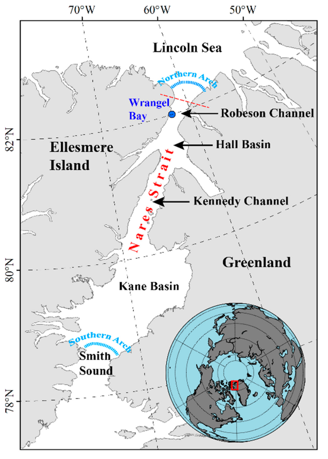
Figure 2.
Daily ice floe speed from Sentinel-1 images and the wind speed. (a) The ice floe speed and wind speed from September 2016 to August 2017. (b) The ice floe speed and wind speed from January 2018 to March 2018.
Figure 2.
Daily ice floe speed from Sentinel-1 images and the wind speed. (a) The ice floe speed and wind speed from September 2016 to August 2017. (b) The ice floe speed and wind speed from January 2018 to March 2018.
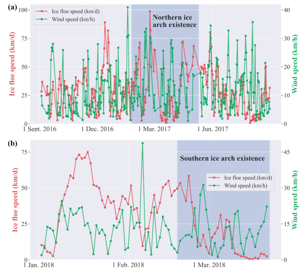
Figure 3.
Wind speed and orientation (3 h) near the north of Hall Basin from 10 December 2016 to 20 December 2016.
Figure 3.
Wind speed and orientation (3 h) near the north of Hall Basin from 10 December 2016 to 20 December 2016.
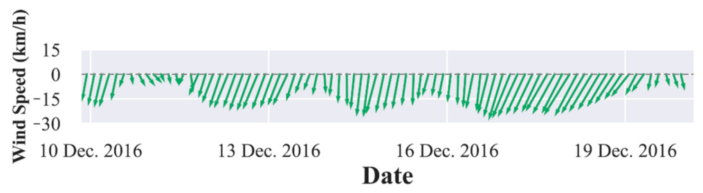
Figure 4.
The process of the breakoff of the consolidated fast ice area attached to the coast of Greenland between 20 and 30 May 2017, after the collapse of the northern arch shown in the image of 14 May 2017. The red triangle marks the area of fast ice area before its breakoff.
Figure 4.
The process of the breakoff of the consolidated fast ice area attached to the coast of Greenland between 20 and 30 May 2017, after the collapse of the northern arch shown in the image of 14 May 2017. The red triangle marks the area of fast ice area before its breakoff.
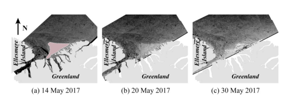
Figure 5.
Wind speed and orientation (3 h) near the northern ice arch from 15 May 2017 to 3 June 2017.
Figure 5.
Wind speed and orientation (3 h) near the northern ice arch from 15 May 2017 to 3 June 2017.

Figure 6.
(a–c) Scatter plots of the ice floe speed calculated from Sentinel-1 versus the speed obtained from sea ice motion products. The diagonal dashed lines are the 1:1 lines. (d–g) Distributions of the ice motion derived from the three products and the corresponding data from the Sentinel-1 images.
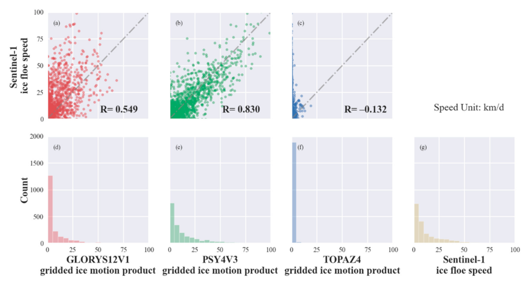
Figure 7.
Kernel density of the deviation in the sea ice motion products (a) GLORYS12V1, (b) PSY4V3, and (c) TOPAZ4 from the ice floe speed extracted from Sentinel-1.
Figure 7.
Kernel density of the deviation in the sea ice motion products (a) GLORYS12V1, (b) PSY4V3, and (c) TOPAZ4 from the ice floe speed extracted from Sentinel-1.

Figure 8.
Rose diagrams for inside and outside the Robeson Channel for (a,d) all the ice floes from Sentinel-1, (b,e) the corresponding ice motion from the GLORYS12V1 product, and (c,f) the corresponding ice motion from the PSY4V3 product.
Figure 8.
Rose diagrams for inside and outside the Robeson Channel for (a,d) all the ice floes from Sentinel-1, (b,e) the corresponding ice motion from the GLORYS12V1 product, and (c,f) the corresponding ice motion from the PSY4V3 product.

Figure 9.
Grouped scatter plots of the ice floe speed from Sentinel-1 versus the speed from the two assessed sea ice motion products (a,c,e) GLORYS12V1 and (b,d,f) PSY4V3. Data in the top, middle and bottom rows are extracted from periods of no arch, northern arch, and southern arch, respectively. The diagonal solid gray lines are the 1:1 lines. The dashed black lines are the fitting lines.
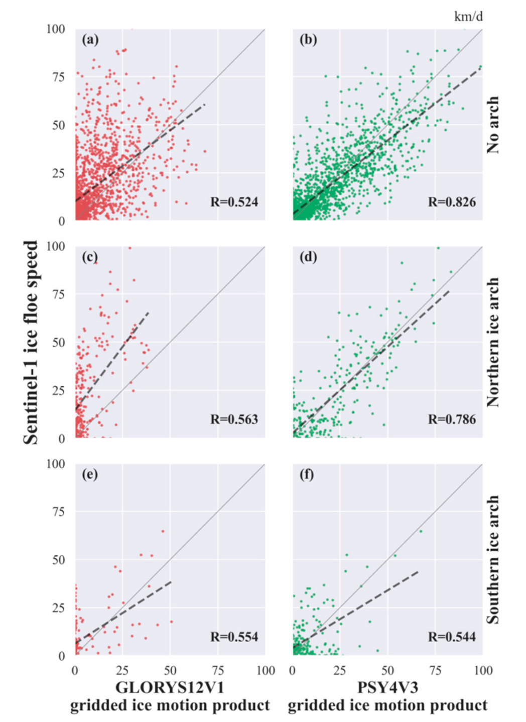
Figure 10.
Variations in the mean absolute errors of the sea ice motion products versus the ice floe speed from Sentinel-1 with changes in ice speed.
Figure 10.
Variations in the mean absolute errors of the sea ice motion products versus the ice floe speed from Sentinel-1 with changes in ice speed.
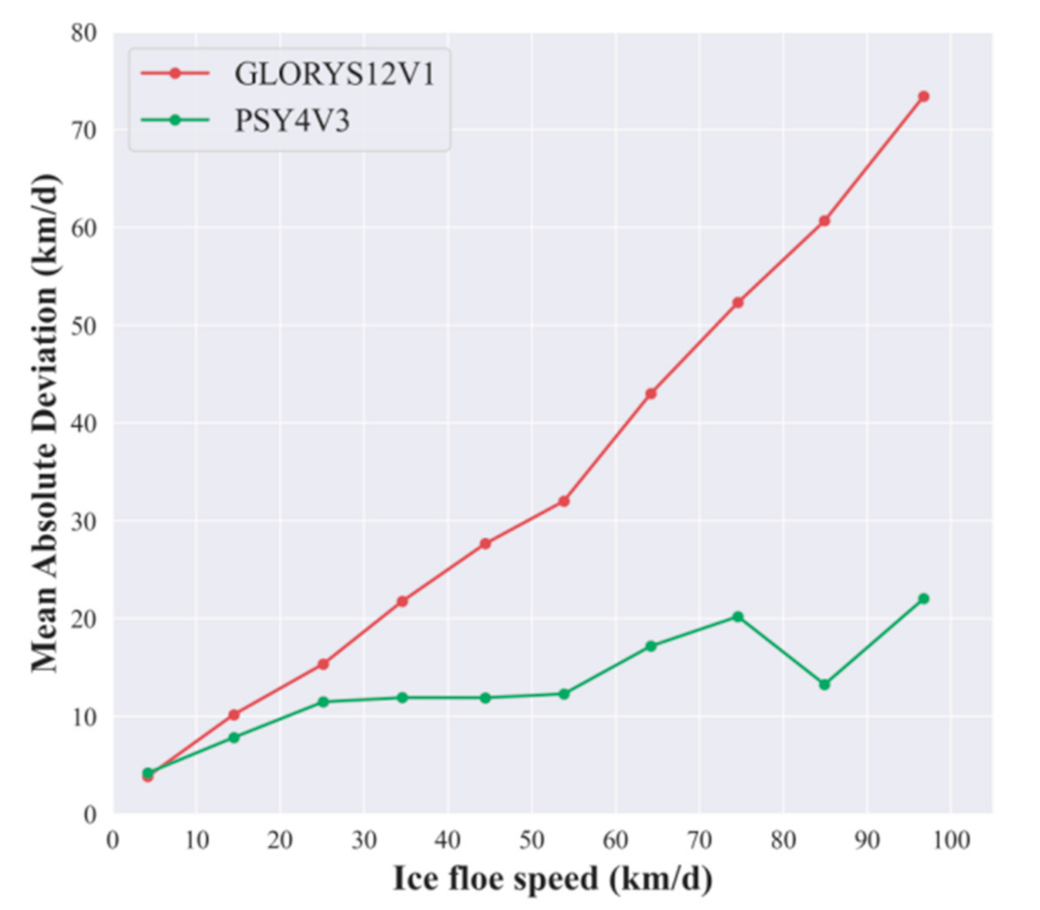
Figure 11.
Daily tidal range and ice floe speed from Sentinel-1 images inside the Robeson Channel (2016–2017).
Figure 11.
Daily tidal range and ice floe speed from Sentinel-1 images inside the Robeson Channel (2016–2017).
Figure 12.
Daily tidal range and deviation between the sea ice motion products and the ice floe speed from Sentinel-1 images inside the Robeson Channel (2016–2017).
Figure 12.
Daily tidal range and deviation between the sea ice motion products and the ice floe speed from Sentinel-1 images inside the Robeson Channel (2016–2017).
Figure 13.
Sea ice conditions in the north of the Robeson Channel on different days during the 2016–2017 sea ice season.
Figure 13.
Sea ice conditions in the north of the Robeson Channel on different days during the 2016–2017 sea ice season.
Figure 14.
Distributions of the deviation of the sea ice motion products for the sea ice floes inside and outside the Robeson Channel.
Figure 14.
Distributions of the deviation of the sea ice motion products for the sea ice floes inside and outside the Robeson Channel.
Figure 15.
Spatial distribution of the relative deviation of (a) the GLORYS12V1 product and (b) the PSY4V3 product, compared with the Sentinel-1-estimated ice floe speed data inside and outside the Robeson Channel. The dots with different colors indicate the different deviation ranges. The black dotted line indicates the entrance from the Lincoln Sea to the Robeson Channel, which separates the two sub-regions. The dotted box indicates Hall Basin.

Table 1.
Basic specifics of the three sea ice motion products assessed in this study.
| Product | Source | Data Source | Methods | Spatial Resolution | Temporal Resolution | Period |
|---|---|---|---|---|---|---|
| GLORYS12V1 | CMEMS | CORA 4.1 T/S, NOAA SST, and CERSAT SIC | NEMO3.1 + LIM2 EVP | 1/12° | Daily | 1993–2019 |
| PSY4V3 | CMEMS | CORA 4.1 T/S, OSTIA SST, and OSI-450/430 SIC | NEMO3.1 + LIM2 EVP | 1/12° | Daily | 2016–2021 |
| TOPAZ4 | ARC MFC | QuickSCAT, AMSR-E, and SSM/I, IFREMER/CERSAT | HYCOM 2.2 + EVP sea ice model | 0.125° | Daily | 1991–2019 |
Table 2.
Monthly samples of ice floes extracted from the Sentinel-1 images for the regions inside and outside the Robeson Channel.
Table 2.
Monthly samples of ice floes extracted from the Sentinel-1 images for the regions inside and outside the Robeson Channel.
| Location | September 2016 | October 2016 | November 2016 | December 2016 | January 2017 | February 2017 | March 2017 | April 2017 |
|---|---|---|---|---|---|---|---|---|
| Outside the Robeson Channel | 24 | 400 | 229 | 83 | 62 | 29 | 15 | 14 |
| Inside the Robeson Channel | 19 | 112 | 72 | 91 | 122 | 39 | 45 | 72 |
| May 2017 | June 2017 | July 2017 | August 2017 | January 2018 | February 2018 | March 2018 | ||
| Outside the Robeson Channel | 48 | 37 | 37 | 24 | 165 | 53 | 86 | |
| Inside the Robeson Channel | 51 | 64 | 71 | 38 | 141 | 73 | 64 |
Table 3.
Correlation coefficient (R) values between the ice floe drift and the sea ice motion products under different conditions in the Robeson Channel.
Table 3.
Correlation coefficient (R) values between the ice floe drift and the sea ice motion products under different conditions in the Robeson Channel.
| Products | All Conditions | No Ice Arch | Northern Ice Arch | Southern Ice Arch |
|---|---|---|---|---|
| GLORYS12V1 | 0.549 | 0.524 | 0.563 | 0.554 |
| PSY4V3 | 0.830 | 0.826 | 0.786 | 0.544 |
Table 4.
Accuracies of the sea ice motion products under the two wind speed regimes separated by the median wind speed of 9.86 km/h.
Table 4.
Accuracies of the sea ice motion products under the two wind speed regimes separated by the median wind speed of 9.86 km/h.
| Wind Speed< 9.86 km/h (Mean Speed of Ice Floe = 16.22 km/d) | Wind Speed> 9.86 km/h (Mean Speed of Ice Floe = 17.12 km/d) | Difference (>9.86 Minus <9.86) | ||
|---|---|---|---|---|
| GLORYS12V1 | MAE | 9.99 km/d | 12.91 km/d | 2.92 km/d |
| RMSE | 14.45 km/d | 20.23 km/d | 5.78 km/d | |
| MAE/mean speed | 61.58% | 73.26% | 11.69% | |
| RMSE/mean speed | 89.07% | 114.81% | 25.74% | |
| PSY4V3 | MAE | 7.48 km/d | 7.31 km/d | −0.16 km/d |
| RMSE | 10.95 km/d | 11.10 km/d | 0.15 km/d | |
| MAE/mean speed | 46.10% | 41.50% | −4.60% | |
| RMSE/mean speed | 67.48% | 62.98% | −4.50% |
Table 5.
Accuracies of each product for the two sub-regions inside and outside the Robeson Channel.
| Outside the Robeson Channel (Mean Speed = 7.00 km/d) | Inside the Robeson Channel (Mean Speed = 28.99 km/d) | ||
|---|---|---|---|
| GLORYS12V1 | MAE | 5.24 km/d | 19.00 km/d |
| RMSE | 7.75 km/d | 24.74 km/d | |
| MAE/mean speed | 74.97% | 65.52% | |
| RMSE/mean speed | 110.73% | 85.33% | |
| PSY4V3 | MAE | 3.98 km/d | 11.55 km/d |
| RMSE | 5.82 km/d | 15.10 km/d | |
| MAE/mean speed | 56.93% | 39.83% | |
| RMSE/mean speed | 83.22% | 52.09% |
Publisher’s Note: MDPI stays neutral with regard to jurisdictional claims in published maps and institutional affiliations. |
© 2022 by the authors. Licensee MDPI, Basel, Switzerland. This article is an open access article distributed under the terms and conditions of the Creative Commons Attribution (CC BY) license (https://creativecommons.org/licenses/by/4.0/).
Share and Cite
MDPI and ACS Style
Liu, T.; Wang, Z.; Shokr, M.; Lei, R.; Zhang, Z. An Assessment of Sea Ice Motion Products in the Robeson Channel Using Daily Sentinel-1 Images. Remote Sens. 2022, 14, 329. https://doi.org/10.3390/rs14020329
AMA Style
Liu T, Wang Z, Shokr M, Lei R, Zhang Z. An Assessment of Sea Ice Motion Products in the Robeson Channel Using Daily Sentinel-1 Images. Remote Sensing. 2022; 14(2):329. https://doi.org/10.3390/rs14020329
Chicago/Turabian StyleLiu, Tingting, Zihan Wang, Mohammed Shokr, Ruibo Lei, and Zhaoru Zhang. 2022. "An Assessment of Sea Ice Motion Products in the Robeson Channel Using Daily Sentinel-1 Images" Remote Sensing 14, no. 2: 329. https://doi.org/10.3390/rs14020329
Note that from the first issue of 2016, this journal uses article numbers instead of page numbers. See further details here.