Article

Development of a Pixel-Wise Forest Transmissivity Model at Frequencies of 19 GHz and 37 GHz for Snow Depth Inversion in Northeast China

1
Northeast Institute of Geography and Agroecology, Chinese Academy of Sciences, No.4888 Shengbei Street, Changchun 130102, China
2
College of Resources and Environment, University of Chinese Academy of Sciences; Beijing 100049, China
3
Changchun Jingyuetan Remote Sensing Experiment Station, Chinese Academy of Sciences, Changchun 130102, China
4
School of Statistics and Data Science, Nanjing Audit University, No. 86 Yushan Western Road, Nanjing 211815, China
5
Shandong Geographical Institute of Land Spatial Data and Remote Sensing Technology, Jinan 250002, China
*
Author to whom correspondence should be addressed.
Remote Sens. 2022, 14(21), 5483; https://doi.org/10.3390/rs14215483
Submission received: 11 September 2022 / Revised: 15 October 2022 / Accepted: 25 October 2022 / Published: 31 October 2022

Abstract

:
Satellite passive microwave remote sensing has been extensively used to estimate snow depth (SD) and snow water equivalent (SWE) across both regional and continental scales. However, the presence of forests causes significant uncertainties in the estimations of snow parameters. Forest transmissivity is one of the most important parameters for describing the microwave radiation and scattering characteristics of forest canopies. Although many researchers have constructed models for the functional relationship between forest transmissivity and forest vegetation parameters (e.g., stand growth and accumulation), such relationships are strongly limited by the inversion accuracy of vegetation parameters, forest distribution types, and scale-transformation effects in terms of regional or global scale applications. In this research, we propose a pixel-wise forest transmissivity estimation model (Pixel-wise γ Model) based on long-term series satellite brightness temperature (TB) data for the satellite remote sensing inversion of snow parameters. The model performance is evaluated and applied in SD inversion. The results show that the SD inversion errors RMSE and Bias are 9.8 cm and −1.5 cm, respectively; the SD inversion results are improved by 41% and 84% after using the Pixel-wise γ Model, compared with the forest transmissivity model applied in the GlobSnow v3.0 product. The proposed forest transmissivity model does not depend on forest cover parameters and other ground measurement parameters, which greatly improves its application scope and simplicity.

1. Introduction

The high-precision inversion of snow depth (SD) and snow water equivalent (SWE) in forest areas is a difficult and open problem in the field of snow remote sensing. Optical remote sensing has advantages for high-resolution mapping of snow covered areas, but it is powerless in the estimation of SD/SWE, and even more so, for the detection of snow under forests, and is also susceptible to cloud influence [1,2]. Passive MicroWave (PMW) remote sensing has unique advantages for SD and SWE inversion and mapping, but mainstream PMW snow remote sensing products, such as the Advanced Microwave Scanning Radiometer 2 (AMSR-2) SD product from the Global Change Observation Mission 1st-Water [3] and the Global Snow Monitoring for Climate Research (GlobSnow) SWE product from the European Space Agency [4,5,6], have not achieved satisfactory accuracy in forest areas [7,8], and cannot meet the requirements of meteorological, hydrological and climate models. Forest snow has a very complex composition; in addition to snow, it also includes dielectric layers such as surface litter, tundra vegetation, shrubs (clumps), trunk (canopy), branches and leaves. The interaction between layers, as well as their radiation and scattering, are factors of interference modeling and signal decoupling. Therefore, in order to realize the high-precision inversion of snow parameters in forest areas, it is necessary to have a clear understanding of the radiation transmission process and the emission and scattering mechanisms of forest snow coupled systems. Quantitatively exploring the relationship between the geometric parameters (such as tree height, diameter at breast height (DBH), canopy density, gap area, etc.,) and physical parameters (such as temperature, etc.) of the forest canopy medium layer and the characteristics of microwave radiation (such as polarization, frequency, etc.), is helpful to further improve and develop the relevant Radiative Transfer (RT) model and provide theoretical support for the inversion of snow parameters in forest areas.
Snow cover is an important scatterer in PMW remote sensing observation, which attenuates the underlying surface microwave signal received by the sensor. Various other components (SD, snow density, frozen/non-frozen soil, etc.), especially in forest parameters, also affect the brightness temperature measured by satellite sensors, which gives the remote sensing inversion of snow parameters under the forest great uncertainty, which in turn seriously limits the accuracy of traditional algorithm inversions of SD and SWE. Therefore, the decoupling of the forest canopy signal and the underlying surface signal (snow, frozen/non-frozen etc.) is particularly important in microwave radiation modeling. In earlier research, the influence of forest terrain on the inversion accuracy of snow parameters has generally been reduced by simply introducing forest coverage parameters into the algorithm as a correction factor [9,10]. However, due to the simplification of the physical process, the universality of the algorithm is unsatisfactory. In recent years, scholars have made some progress in developing and applying empirical or semi-empirical models (including look-up table method, Bayesian assimilation method, etc.) and complex models considering canopy and trunk scattering/absorption effects [11,12,13], but subject to the acquisition of accurate information parameters of vegetation, this is still a significant challenge in the application of satellite remote sensing inversion [14]. Therefore, simplified RT models, such as τ-ω models, are often used to characterize forest radiative transfer processes [15,16,17]. In PMW satellite signals of the forest snow observation scene, forest radiation is a function of microwave frequency, polarization mode, satellite observation angle and forest effective physical temperature, etc. Among these parameters, forest canopy microwave transmissivity (hereinafter referred to as forest transmissivity) is one of the important parameters for describing the absorbing and scattering characteristics of forests. The question of how to parameterize the forest transmissivity accurately is one of the key points to correct the forest effect, and to realize the high-precision inversion of snow parameters under forests.
Among the SD/SWE inversion algorithms based on RTM in forest areas, the previous transmissivity parametric models are often obtained by establishing empirical or semi-empirical functional relationships based on point scale ground measurement data. For example, microwave transmissivity of forest vegetation has been explored through observation [18,19,20,21,22,23,24] and modeling perspectives [25,26,27], respectively. However, scale conversion is rarely considered; that is, when the point scale is extended to the PMW pixel scale, the applicability of the model is uncertain. For example, although the transmissivity model expressed as a function of Growing Stock Volume (GSV) is applied to GlobSnow products, its uncertainty still increases exponentially with the increase of forest coverage [14]. In view of the above limitations, we need to consider how to parameterize or solve the forest transmissivity directly from the pixel scale.
Zeroth order τ–ω models [15,16,17] aim to simplify complex microwave tree interactions into robust, tractable equations, requiring only a small number of parameters, and thereby making them suitable for large-scale applications, especially when there is insufficient auxiliary data, such as canopy structure, that can support higher-order models. Based on the τ–ω model, this study develops a Pixel-wise model to estimate the winter forest transmissivity of horizontal (H) and vertical (V) polarizations at frequencies of 19 GHz and 37 GHz for each year of 2014–2019 in forest area of Northeast China. The model performance is evaluated, and forest transmissivity data sets are applied in SD inversion, and satisfactory results are obtained.

2. Study Area and Data Set

2.1. Study Area

Northeast China (38°72′–53°55′ N, 115°09′–135°52′ E) is located in the mid-latitude of the northern hemisphere, covering a total area of approximately 1.2 million km2 and with an elevation range of 0–2667 m. The climate of Northeast China is controlled by the high latitude East Asian monsoon, which includes warm temperate and cold temperate zones latitudinally, as well as semi-arid, semi-humid and humid zones from west to east. The geographical location and climatic conditions of this region creates a relatively complex surface cover system. According to the GLC_FCS30-2015 global land-cover products [28] (free access at https://doi.org/10.5281/zenodo.3986872, accessed on 8 July 2020), Northeast China is dominated by forests, croplands and grasslands, as shown in Figure 1a, accounting for about 40.4%, 36.9% and 13.1% of the total area, respectively. Forest cover is widely distributed in the mountainous areas, including the Greater Khingan Mountains, Lesser Khingan Mountains and Changbai Mountains areas [29]. The forest cover fraction data within each passive microwave satellite pixel (25 km × 25 km) are calculated (Figure 1b). The areas of deciduous broad-leaved forests and deciduous coniferous forests of forestry land in Northeast China are superior, which are 73.1% and 22.4% of the total, respectively. In addition, Northeast China is one of the three primary snow-covered regions (Xinjiang, Northeast China and the Qinghai-Tibet plateau) in China [30,31]. In winter, snowfall is frequent and evenly distributed, and snow cover lasts from November until April. The maximum snow depth (MSD) in Northeast China forest area generally shows a spatial distribution characteristic, gradually deepening from southwest to northeast, with variations ranging from 5–9 cm incrementally to 21–32 cm [32]. Rich snow resources and forest diversity make Northeast China an ideal region for forest snow research.

2.2. Input Data for Forest Microwave Transmissivity Modeling

The investigation period is from September 2014 to March 2019, covering five winter freezing seasons across Northeast China.

2.2.1. SSMIS Brightness Temperature

Time series TB data from the SSMIS sensor currently operating on board the Defense Meteorological Satellite Program (DMSP) spacecraft F17 were used for solving the transmissivity of 19 GHz and 37 GHz in Northeast China’s forested areas. The TBs at 19, 37 and 91 GHz were obtained from the National Snow and Ice Data Center (NSIDC, https://nsidc.org/data/NSIDC-0032, accessed on 31 July 2019) at the EASE Grid format, with a nominal resolution of 25 km × 25 km [33]. The dynamic range of TBs is 55–320 K, and the ground observation angle is 53.1°. To match the spatial scale of different remote sensing products, the original TB data set was resampled into a standard latitude and longitude gridding (0.25° × 0.25°) format. Only descending (approximately 05:00–07:00, local time) orbital data was applied for reducing the uncertainty caused by wet snow and atmospheric turbulence. The TB values with sudden unrealistic temporal changes had been filtered out according to the criterion d TB > 3 Std ( d TB ) , meaning TBs are chosen as normal values within three standard deviations.

2.2.2. ERA5-Land Daily Air Temperature Data

ERA5-Land is an updated version repeated after a series of improvements based on the reanalysis data of ERA5, with higher spatial resolution (9 km in ERA5-Land vs 31 km in ERA5), and the time span has been from January 1950 to now. The ERA5-land product was generated on the basis of the ERA5 climate dataset by the European Centre for Medium-range Weather Forecasts (https://cds.climate.copernicus.eu/, accessed on 10 June 2021). In this study, the daily air temperature elements (Unit: K) at 2 m from ERA5-Land data set were used, which refers to the air temperature at 2 m above the surface of land and is obtained by interpolating between the lowest layer of the model and the Earth’s surface. Due to the different spatial resolutions of SSMIS (standard latitude and longitude gridding 0.25° × 0.25°) and ERA5-Land (0.1° × 0.1°), the ERA5-Land air temperature product was resampled to the same spatial size as SSMIS. The processing operations of re-griding were necessary for aligning all relevant information sources, including forest cover fraction, land cover type, ERA5-Land derived air temperature, TB observations and Pixel-wise transmissivity model outputs on a coincident grid.

2.3. Validation Data

2.3.1. Microwave Transmissivity Measurement Data

In mid-to-late December 2016, we conducted a series of ground-based microwave radiometric observation experiments in the forest. Downwelling TBs at 19- and 37-GHz for horizontal and vertical polarizations from the forest canopy were measured at 14 tree sample plots using microwave radiometers. The geographical location of the radiometric sites are shown in the red triangle in Figure 1b. Based on the measured data of TBs and air temperature, combined with the sky background TBs data, the in-situ forest transmissivity for each frequency and polarization was calculated, following the simplified approach provided by [19]. A further detailed description of this dataset can be found in [24]. In this study, this dataset is considered as a reference for the actual value of ground measurements of forest transmissivity.

2.3.2. China’s Snow Survey Data

China’s snow survey (also known as Investigation on Characteristics and Distribution of Snow Cover in China) data sets were collected from a total of six snow measuring lines, as well as several quadrats and stations, spanning across Northeast China, Xinjiang, and Qinghai-Tibet plateaus, during the winter period of 2017–2019 [34,35]. In this study, only the line measurement dataset in Northeast China was used, and the experimental area was mainly distributed around the Greater Khingan Mountains, Lesser Khingan Mountains, Sanjiang Plain, Songneng Plain and Changbai Mountains. The entire snow season was divided into three periods, with reference to snowfall frequency and the surface snow accumulation state: accumulation period, stabilization period and melting period, which lasted for two years; the observations were repeated three times a year. The distribution of snow pit sampling sites is illustrated via the blue ink dots in Figure 1b. As of 18 March 2019, 443 snow pit sample sites were collected in Northeast China, of which 329 were located in SSMIS pixels, meeting the condition of forest cover fraction ≥10%. Snow pit profile measurement parameters mainly include SD, snow grain size, snow layer dielectric constant, snow liquid water content, snow layer hardness, snow layer temperature, stratified snow density and overall snowpack density.

3. Models and Methodology

3.1. Zeroth Order τ–ω Radiative Transfer Model

The TB above the forest canopy at certain nadir angles (e.g., 53.1° for SSMIS observations), and with different frequencies and polarizations, can be modeled using a simple microwave vegetation radiative transfer model called the τ–ω model, which calculates the following main contributions (ignoring the subtle atmospheric emission reflected by the underlying surface) as:
T B , a c f , p = T B , underlying f , p + T B , forest f , p + T B , f o r e s t r f , p
where T B , a c f , p is the upwelling microwave emission (unit: K) above forest canopy measured by satellite sensor; T B , underlying f , p is the upwelling emission (unit: K) of the underlying surface (containing soil and snow); T B , forest f , p is the upwelling emission (unit: K) of the forest canopy; T B , f o r e s t r f , p is the downwelling forest vegetation emission (unit: K) reflected by the underlying surface; superscript f represents frequencies 19 and 37 GHz in this study; superscript p is the vertical (V) or horizontal (H) polarization. Following the theory and method proposed by Mo et al. (1982) [15], with vegetation scattering and transmission coefficient (τ–ω) and ground emissivity, Equation (1) can be further expressed as:
T B , a c f , p = γ E f , p T u n d e r l y i n g + 1 ω f , p 1 γ f , p T forest + 1 ω f , p 1 γ f , p γ f , p 1 E f , p T forest
γ f , p = exp τ f , p cos 1 θ
where E is the emissivity of the underlying surface (unitless), T u n d e r l y i n g is the effective underlying surface temperature (unit: K), and T forest is the forest vegetation temperature (unit: K). ω is the forest single-scattering albedo (unitless); γ is the effective forest transmissivity (unitless)which can be represented by the effective forest vegetation optical depth τ, as shown in Equation (3) and θ is the incidence viewing angle toward nadir of the radiometer (unit: Rad).
The parameter E is linked to the dielectric properties of the underlying surface, which are significantly influenced by properties of the ensemble medium, such as soil moisture and various features of snow medium covering the ground, including snow depth, volume fraction, wetness, snow cover fraction [36,37,38], etc. As E is generally unknown, the parameters τ and ω are difficult to retrieve directly from the above equations [15,34]. Nevertheless, the parametric solution for τ (or γ) is achievable under some reasonable assumptions. Due to the relatively small magnitude of ω, we assumed ω to be negligible for this study according to literature practices [39,40,41]. In addition, most previous studies [11,19,42,43,44,45] assumed that T a i r T forest T G r , thereby Equation (2) yields to a simplified relationship:
T B , a c f , p = 1 γ f , p 2 1 E f , p T f o r e s t
Further, the solution of γ is:
γ f , p = T f o r e s t T B , a c f , p 1 E f , p T f o r e s t
In the following, we solved Equation (5) to derive γ at the satellite pixel scale.

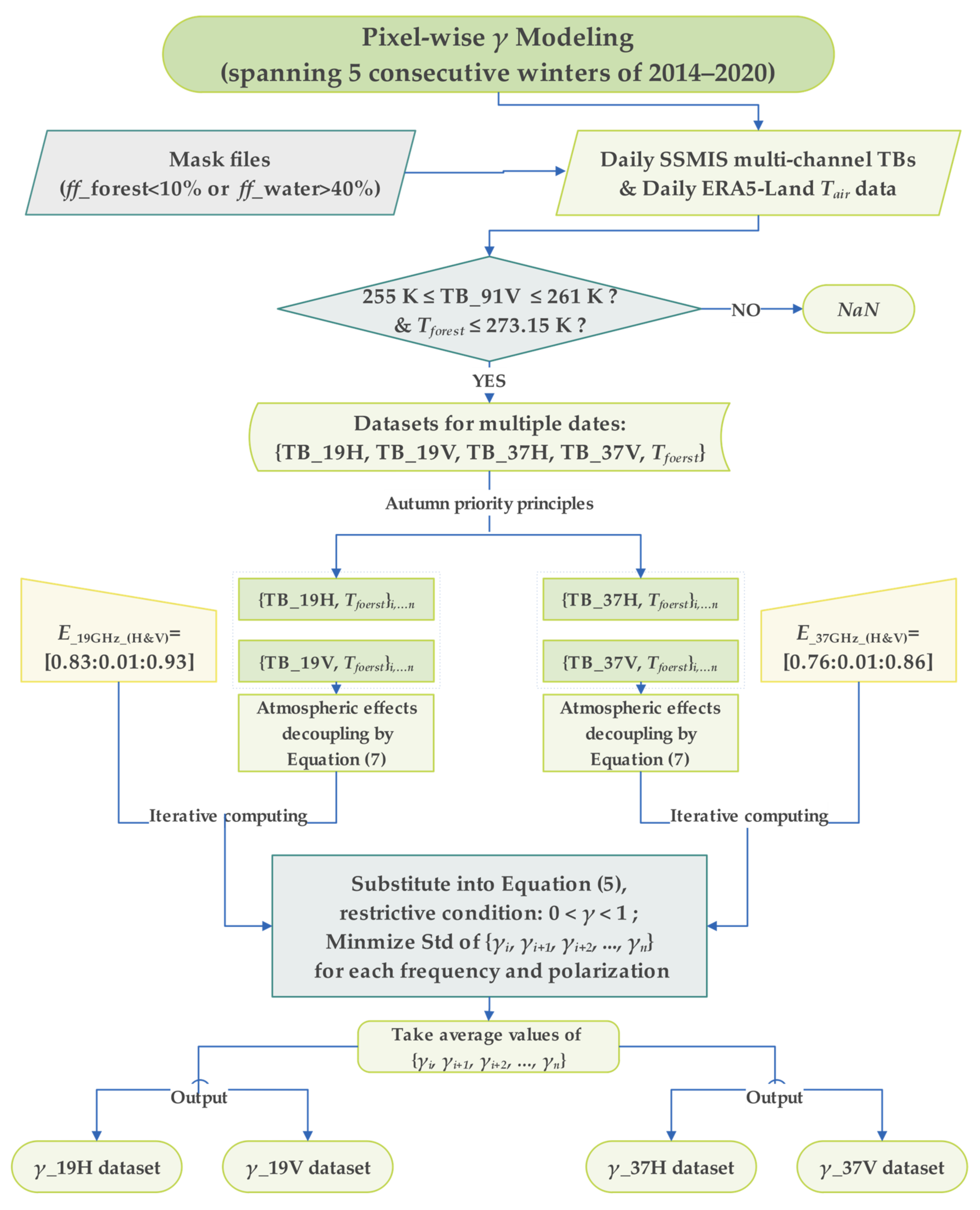
3.2. Pixel-Wise Forest Microwave Transmissivity Modeling

Owing to the large heterogeneity in land surface types within the coverage range of satellite pixels, the retrieved values of forest transmissivity are considered as the “effective transmissivity” at the pixel scale, rather than that at the forest plot scale, which also implies that the outputs of the Pixel-wise forest microwave transmissivity model (hereafter referred to as the “Pixel-wise γ Model”) are not dependent on the forest cover fraction parameter. To build the Pixel-wise γ Model, the following assumptions are given based on the foundation of previous research, in addition to those mentioned in Section 3.1:
(1)
Snow characteristics, effective permafrost emissivity and other environmental parameters are considered to be approximately the same for forest and non-forest areas within the same pixel and are set to equal values in the modeling [43];
(2)
The value of Pixel-wise γ remains almost constant during each winter season (September to March of the following year). This assumption is reasonable since previous studies [40,43,46] usually assumed that the winter γ at 19 and 37 GHz remains fixed over a more extended time period (generally the period of growth cycles in forest growing stock or aboveground biomass).
A flowchart of the modeling Pixel-wise γ for all four frequency and polarization combinations (19 GHz and 37 GHz, H and V polarizations) in freezing conditions is presented in Figure 2.
Three primary steps are included in the retrieval scheme.
Step 1: Determine the dates of a subset of stable dry snow conditions
Considering the feature matching accuracy error of land cover type data products and the improvement of computational efficiency, we took the lead in filtering out pixels with <10% forest cover (i.e., ff_forest <10%); meanwhile, to avoid the retrieval error caused by water bodies and wetlands, we excluded pixels with a total coverage of more than 40% water bodies (i.e., ff_water >40%).
From Equation (5), it can be deduced that the γ retrieval necessarily requires the determination of three parameters, T B , a c f , p , E f , p and T f o r e s t . The parameters T B , a c f , p and T f o r e s t were obtained from the time-series SSMIS TB data and the ERA5-Land air temperature products, respectively, while parameter E f , p needs to be qualified by setting a threshold condition. As aforementioned, E f , p is related to the underlying surface dielectric properties, and therefore the fluctuation range of E f , p for a relatively stable soil/snow state should theoretically be relatively insignificant. Consequently, our primary effort is to determine a relatively stable period or date of the underlying surface state, with a view to providing a constraint on E f , p . Thus, we proposed a rule for determining the dates of soil freezing with dry snow cover by referring to the identification algorithm mentioned in the snow product production specification of AMSRE [47]:
255   K T B _ 91 V 261   K & T f o r e s t 273.15   K ,
where T B _ 91 V is the TB values (unit: K) at 91 GHz V polarization channel, and T f o r e s t is the air temperature (unit: K). The range of values for E f , p will be given in Step 2.
After searching pixel by pixel, and day by day, the datasets ({TB_19H, TB_19V, TB_37H, TB_37V, Tfoerst}) of multiple dates that satisfy the above conditions were acquired. To circumvent the influence of microstructural properties of deep or wet snow (which usually occurs in late winter and early spring) on TBfor example, deep snow weakens the emissivity ( E f , p ) while wet snow enhances it, leaving it in a highly unstable statethe “autumn priority principle” as the screening condition was proposed. Specifically, for those that meet the above discriminatory conditions of Equation (6), we give priority to the data set ({TB_19H, TB_19V, TB_37H, TB_37V, Tfoerst}) in autumn, and the eligible data set before December 31 of each year will be chosen and input to the model.
Since the influence of the atmosphere on the measured PMW TB is particularly pronounced when observations are made at high frequency microwaves (i.e., greater than 10 GHz) [48], the atmospheric decoupling of TBs at 19 GHz and 37 GHz is required. Following the simplified approach [44,49], the corrected TB ( T B , n o a t m ) from the satellite measurements can be derived:
T B , n o a t m = T B , s a t T B , a t m t a t m
where T B , n o a t m (unit: K) corresponds to the parameter T B , a c f , p in Equation (5), T B , s a t represents the TB values (unit: K) acquired from SSMIS, T B , a t m is the upward atmospheric radiations (unit: K) and t a t m is the atmospheric transmissivity (unitless). The parameters T B , a t m and t a t m can be obtained from the atmospheric statistical model [50,51], which will be given in Section 3.3.2.
Step 2: Determine the effective emissivity of dry snow-covered frozen ground
In step 1, we have screened out the state period/date that satisfies the condition (Equation (6)) that the soil is frozen and covered with dry snow, pixel by pixel. Next, we need to determine the range of values for parameter E f , p of the underlying surface in this state. Therefore, it needs to be particularly explicit that E f , p here refers to the “effective emissivity”, meaning the underlying surface containing both snow medium and frozen soil medium is regarded as an integrated medium. Previous studies on the emissivity of snow-free frozen ground or snow surface have been conducted to show that: (1) Based on radiometric experiments in the farmland area of Northeast China, Wu et al. (2017) [52] measured the emissivity of snow-free frozen ground of 19 GHz and 37 GHz horizontal polarization to be 0.92 and 0.93, respectively; (2) Mätzler (1994) [53] pointed out that the polarization difference of permafrost emissivity is very small, and the polarization difference of 19 GHz and 37 GHz is 0.0068 and 0.0009, respectively. (3) Snow emissivity can vary from 0.4 to 1.0 due to complicated snow properties [53,54,55]; (4) Yan and Weng (2003) [56] retrieved the time series of globally mean land emissivity at all of seven SSM/I channels, during 1993–2002, over snow surface, giving the monthly mean emissivity with the value of 0.81, 0.91, 0.75 and 0.84 for 19 GHz (H), 19 GHz (V), 37 GHz (H) and 37GHz (V), respectively. Since the difference in emissivity polarization at the pixel level is not completely clear, this study directly selects the average value at dual polarization of each frequency band as the upper and lower limits of the threshold condition to participate in the model run. In addition, taking into account the complexity of the radiation characteristics of the forest floor, and referring to the results of preliminary trial calculation of the model, we set E f , p as (increment is set to 0.01):
E _ 19   G H z _ ( H a n d V ) = 0.83 :   0.01 :   0.93
E _ 37   G H z _ ( H a n d V ) = 0.76 :   0.01 :   0.86
So far, three input parameters ( T B , a c f , p , T f o r e s t and E f , p ) of the Pixel-wise γ Model have been determined. Following this, substitute Equations (8) and (9) and the filtered data set ({TB_19H, TB_19V, TB_37H, TB_37V, Tforest}) from Step 1 into Equation (5) for iterative operations.
Step 3: Iterative optimization
By processing the first two steps, a matrix of γ retrieval values was generated pixel by pixel. Using hypothesis (2) in Section 3.2 that the Pixel-wise γ retrieved value remains almost unchanged in the winter snow period of each year, the optimization criterion, namely, the standard deviation (Std) of the changing sequence γ, should be minimal. In addition, it is necessary to add the restriction: 0 < γ < 1, to ensure the validity of γ in the iterative process. Ultimately, a multi-day γ series with minimum Std was picked in the matrix and averaged as the model output, i.e., the γ retrieval value.

3.3. Evaluation Approaches

To validate the output of the Pixel-wise γ Model at the satellite pixel scale (~25 km × 25 km), we proposed two validation schemes: one was to directly compare the “model output” with the “true value” using a limited number of measured γ data, and the other was to retrieve snow parameters (including SD and SWE) by embedding the Pixel-wise γ Model into the radiative transfer model system in order to complete indirect validation. The commonly used root mean-square error (RMSE), Bias and correlation coefficient (r) were used as evaluation metrics.

3.3.1. Direct Validation with Measured Data of Transmissivity

Due to spatial scale effects, the difficulty of verifying the retrieved values of γ at the pixel scale using the measured sample point data is undoubtable. Nevertheless, the measured data can visualize the reliability of the retrieved dataset in some ways. The forest microwave transmissivity measurement dataset contained 14 sample sites cumulatively, corresponding to being encapsulated in 8 SSMIS pixels, i.e., some pixels cover 2–3 sample sites. For the calculation of γ in multiple-site pixels, the average value was used. The reliability of the model output dataset is evaluated by directly comparing the difference between the measured and retrieved values.

3.3.2. Indirect Validation with Retrieval of SD and SWE

It is known that the removal of forest effects in the manufacturing framework of the Globsnow SD/SWE product [5,6,57] is based on the τ–ω model, with integrating the forest γ model into the overall RT modeling system. Following the modeling idea of Globsnow, we note that the Pixel-wise γ Model can also be easily incorporated into a snow emission model, such as the HUT model [58], to account for microwave attenuation in a forest canopy. Thus, the indirect validation can be achieved by replacing the parameter γ in the module of its RT modeling system and comparing the SD/SWE retrieval accuracy. Both direct forward modeling of SSMIS TB using in situ data for properties of snow cover and the inversion of forward models to retrieve SD/SWE were applied in this study. Note that, whilst we applied the forward model provided by the GlobSnow SWE product (v3.0), we used a different inversion algorithm (different cost function) to GlobSnow. The forward model information for the satellite measurement of TB simulations was summarized in Table 1.
The atmospheric models used in this study included two types: a physical model with sounding data as input, i.e., the Millimeter Propagation Model (MPM) developed by Liebe (1989) [59], and the other model proposed by Pulliainen et al. (1993) [51], which was an empirical model based on statistical data. However, considering that actual atmospheric measurement data are difficult to obtain simultaneously over a large area, we modified the Atmospheric Statistical Model (ASM) using the MPM model for the practical needs of reducing the computational effort and simplicity of application. The specific expression of the ASM is as follows:
T B atm , ( ) = α ( ) T a i r 1 t a t m
t a t m = τ a t m ( 1 ) + ζ τ a t m ( 2 )
τ a t m ( 1 ) = [ 0.9851 ; 0.9795 ; 0.9211 ; 0.8326 ; 0.8624 ; 0.6656 ]
τ a t m ( 2 ) = [ 0.0088 ; 0.0275 ; 0.2069 ; 0.4642 ; 0.2746 ; 0.8163 ]
where T a i r is the surface air temperature (unit: K) which can be acquired from ERA5-Land product, α ( ) is the approximate atmospheric profile factor (unitless) to determine the effective temperature [50]; t a t m (unitless) is from statistical results [51,60]; Equations (12) and (13) are given statistical parameters, corresponding to frequencies of 6.9-, 10.65-, 18.7-, 23.8-, 37- and 89 GHz, respectively. ζ is a statistical coefficient that equals 0.0368 when applied in Finland and needs to be recalibrated when used in other regions. Using the MPM model output data set as a reference, we corrected the coefficient ζ from 0.0368 for Finland to 0.2406 for Northeast China by least squares fitting.
Next, it is necessary to parameterize the HUT snow emission model and rough bare soil reflectance model separately, using the pixel observations in the snow survey dataset, which can be referred to [57], where the optimized parameters of the soil model have been listed in Table 1. As for the HUT model, the focus of optimization is on its extinction coefficient, i.e.,
κ e = 8 f 1.5 1 e 1.5 D m 3.7
where f is the frequency (unit: GHz), and D m is the measured snow grain size (unit: mm).
After completing the initialization of the forward model parameters, an iterative process using an increment of 0.1 cm on SD (range: 0–40 cm) and of 0.1 mm on SWE (range: 0–80 mm) was used to retrieve the SD/SWE values, respectively, that minimized the RMSE between the measured (SSMIS) and simulated (simu) TB for incidence angle (θ) of 53° such that:
M i n i m i z e 1 2 σ 2 ( T B , s i m u 19 V T B , s i m u 37 V ) ( T B , S S M I S 19 V T B , S S M I S 37 V ) 2 + ( T B , s i m u 19 H T B , s i m u 37 H ) ( T B , S S M I S 19 H T B , S S M I S 37 H ) 2 + ( T B , s i m u 19 V T B , s i m u 19 H ) ( T B , S S M I S 19 V T B , S S M I S 19 H ) 2 + ( T B , s i m u 37 V T B , s i m u 37 H ) ( T B , S S M I S 37 V T B , S S M I S 37 H ) 2
where σ is the standard deviation of SSMIS measurements, which is assumed to be 2 K, according to the sensitivity characteristics of the SSM/I instrument [62].
Further, we chose the γ retrieval algorithm provided by the GlobSnow 3.0 product (hereafter referred to as the GlobSnow algorithm) as the object of comparison, with all other sub-module input parameters held constant, and only the parameter γ was retrieved by the Pixel-wise γ Model (hereafter referred to as the Pixel-wise algorithm) replaced in the forward model. The dual-frequency dual-polarization γ retrieval formula provided by the GlobSnow algorithm [46] is as follows:
t r a n s v e g = e k e G S V
where k e is the forest vegetation extinction coefficient, which is 0.01, 0.007, 0.012 and 0.011 at 19 GHz and 37 GHz for H and V polarization, respectively; and GSV is the forest stem volume (unit: m3 ha−1), which can be obtained from ESA BIOMASAR [63]. Finally, the Pixel-wise algorithm and the GlobSnow algorithm were applied to solve SD and SWE in reversion, respectively.

4. Results

4.1. Validation Results

4.1.1. Accuracy Validation Based on Measured Transmissivity

The results of the comparison between the retrieved and measured values of γ are shown in Table 2. The examples of γ presented in bold refer to the data points in which the difference between the estimated γ and the measured value with the Pixel-wise γ Model is beyond ±0.1, demonstrating that the estimation accuracy is relatively poor. It can be found that the γ at the individual frequencies/polarizations of the pixels where the sampling points Yichun02, Yichun04, Xunke04, and Yichun01 are located, and the γ at the full frequencies/polarizations of the pixels where the sampling point Yichun03 is located are overestimated, and the estimation accuracy is extremely low. One of the reasons for this phenomenon is that the overall forest density or accumulation on the SSMIS footprint is not as high as the actual measured sample sites, especially for the sample sites in Yichun, where the forest type is evergreen coniferous forest, the γ measurements are relatively low, mostly in the range of 0.2–0.36, which is still far from the saturation value of transmissivity at pixel scale (in the range of 0.5–0.6). This can be explained by the scale effect, as the dominant forest type in the pixel where the sample site located is not evergreen coniferous forest, but deciduous broadleaf forest and mixed forest. In general, the validation accuracy is high for the Huma region, represented by deciduous coniferous forest, and the Xunke region, represented by deciduous broadleaf forest, with an average error of only 0.01, but the validation effect is poor for the Yichun region, represented by evergreen coniferous forest (caused by the mismatch of dominant forest types).

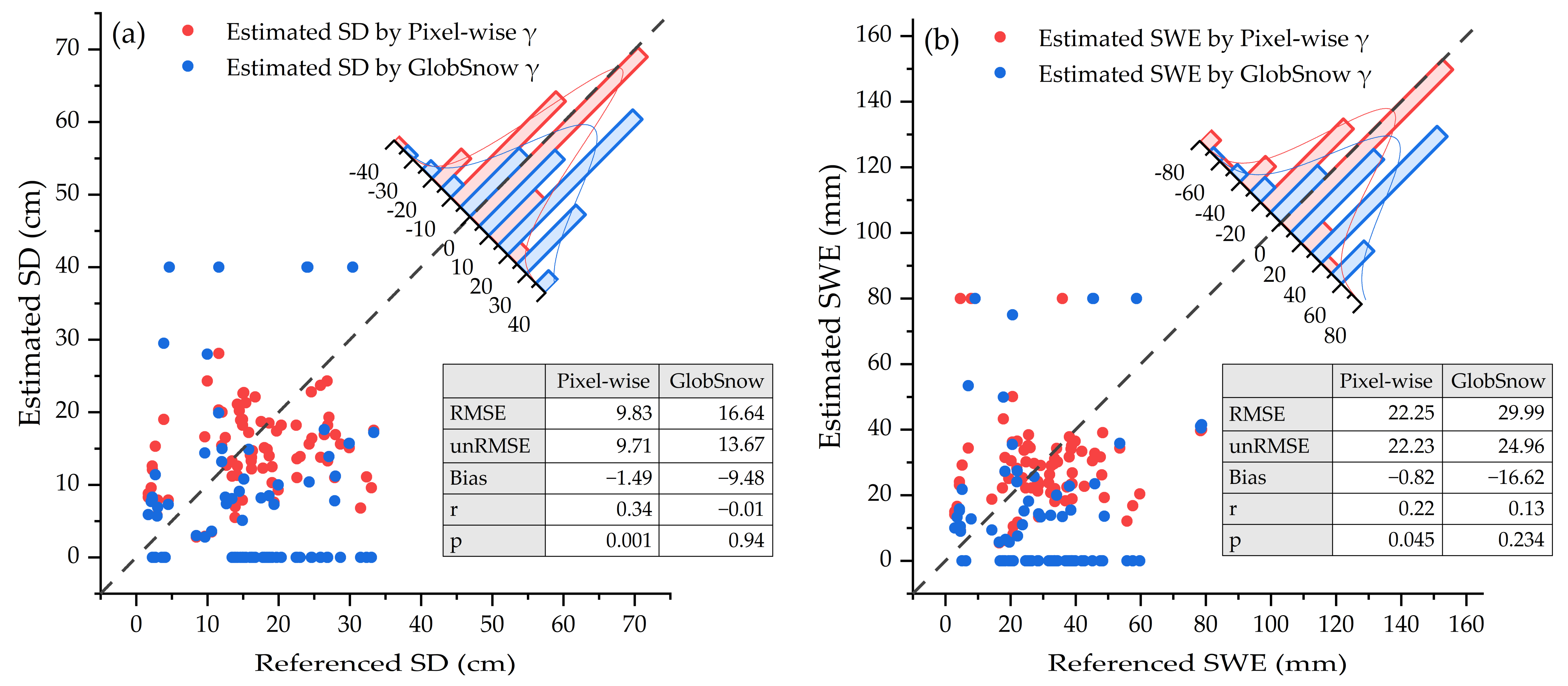
4.1.2. Retrieval of SD and SWE

The SD and SWE results obtained by inversion with the Pixel-wise algorithm and GlobSnow algorithm, respectively, are shown in Figure 3, and the evaluation metrics are also superimposed in Figure 3.
From the graphical results in Figure 3, all evaluation metrics show that the Pixel-wise algorithm has significantly improved accuracy compared with the GlobSnow algorithm. From the index RMSE, the accuracy of SD and SWE inversion is improved by 6.8 cm and 7.75 mm, respectively, with an effective accuracy improvement of 41% and 26%, respectively; from the index Bias, the accuracy of SD and SWE inversion is improved by 84% and 95%, respectively; in addition, the correlation coefficient r is also improved. From the histogram of angular difference (difference = measured value − estimated value) in Figure 3, it can be found that the inversion errors of the Pixel-wise algorithm are mostly concentrated near the 0 point, while the errors of the GlobSnow algorithm are significantly right-skewed, i.e., the measured value is much larger than the estimated value, and the underestimation is severe. It is also found that the SD and SWE values of the inversion performance of the Pixel-wise algorithm have almost no boundary values, so it is more usable than the GlobSnow algorithm for the application in the forest area of Northeast China. In summary, it can be found that the Pixel-wise γ Model is more advantageous than the γ algorithm applied in the GlobSnow product for the inversion of snow parameters in the forest area of Northeast China. The adaptability of the proposed model is basically similar to GlobSnow as it does not depend on regional parameters and can be applied to regions besides Northeast China.

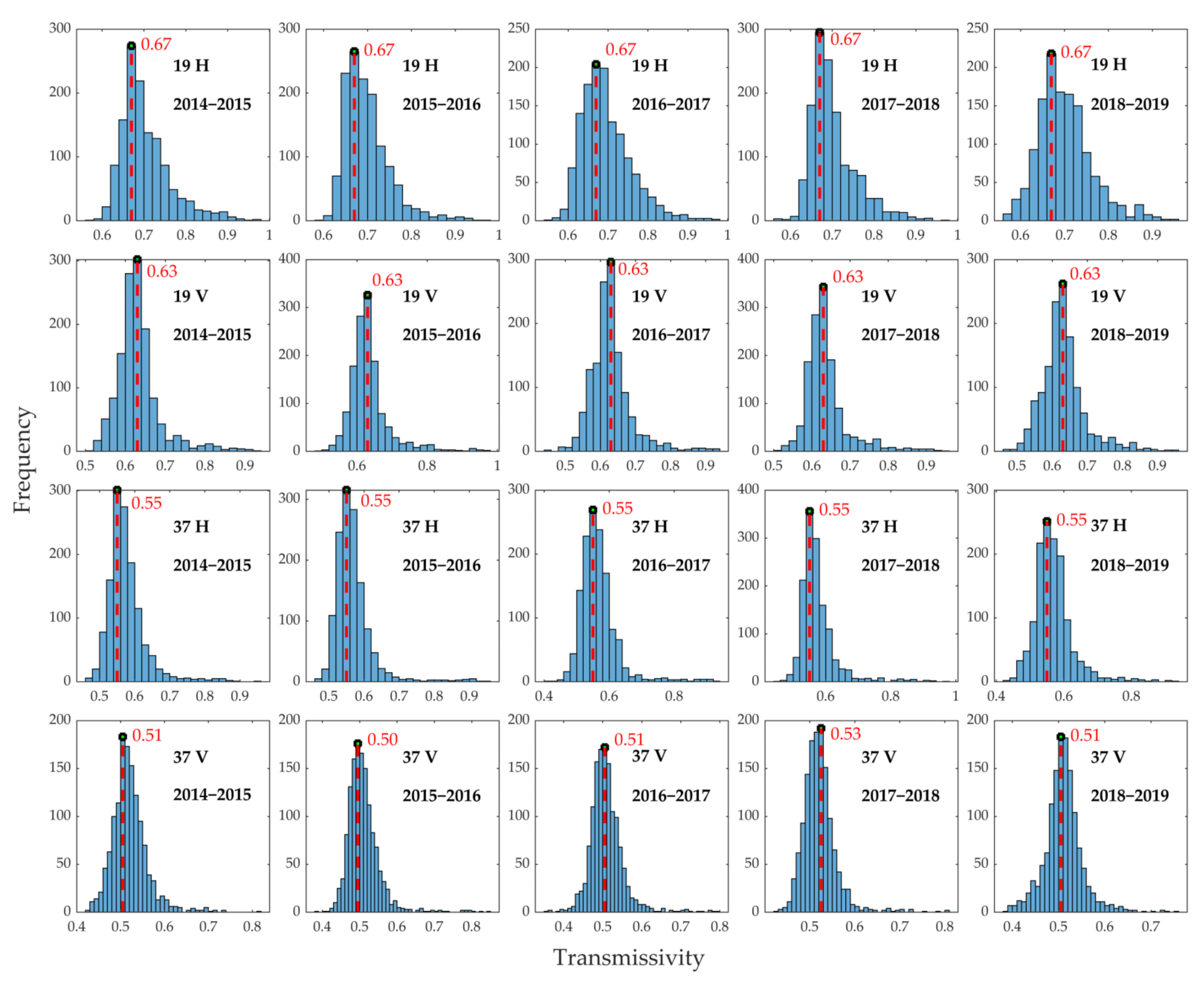
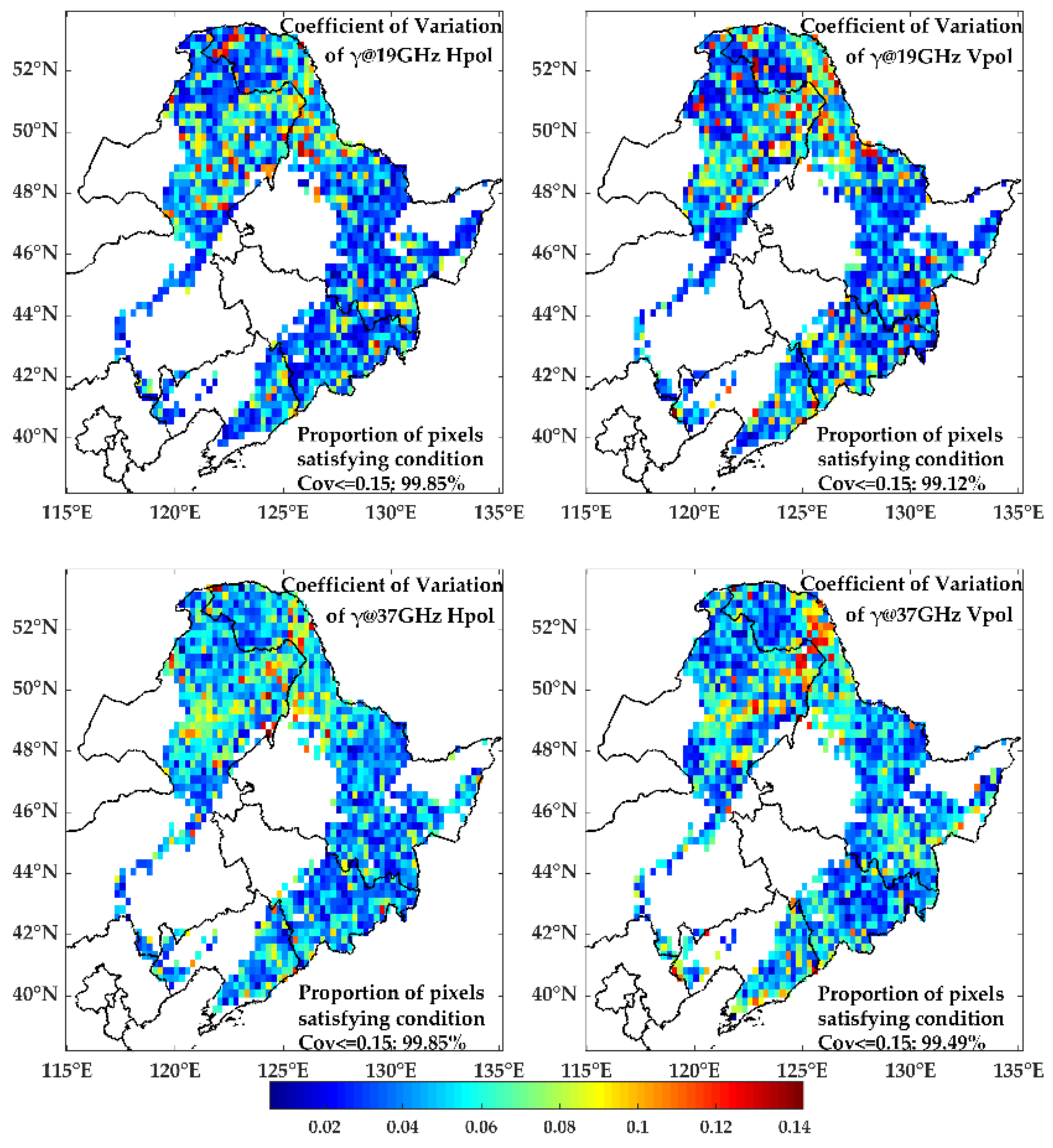
4.2. Spatio-Temporal Distribution Characteristics of Pixel-Wise Transmissivity

The spatial distribution of γ values for the H and V polarizations at 19 GHz and 37 GHz are shown in Figure 4, where the gray grid (with a special setting of 1.00) indicates that the forest pixel does not satisfy the Pixel-wise γ Model constraint, and the retrieved value is invalid. It can be found that the overall results show γ values at 19 GHz is higher than those of 37 GHz and the H polarization is higher than the V polarization. This is consistent with the theory that the penetration depth increases with decreasing frequency [16].
Taking the winter of 2014–2015 as an example, it can be seen that the values of the Pixel-wise γ range from 0.58–0.97 at the 19 GHz H polarization, while the frequency distribution histogram (Figure 5) shows that the values are concentrated in the grouping interval (i.e., the modal interval) of 0.66–0.68, and the value ranges of the frequency and polarization in other years are summarized in Table 3. In addition, it can be seen in Figure 5 that the shape of the overall γ distribution is almost the same for each year, at the same frequency and polarization. The red dashed line in the figure gives the modal values of γ for each year, and it can be seen that the modal values of γ for V and H polarizations at 19 GHz and the H polarization at 37 GHz remain stable and constant for each year, and there are fluctuations of 0.01–0.02 in the modal values of γ for the V polarization at 37 GHz, with relatively small magnitude. As can be seen in Table 3, the center of the γ modal interval undergoes a shift of roughly 0.02–0.03 in the interannual variation, and the range of extremum variations are relatively stable, with fluctuations up to 0.12 under the overall spatial range.
One of the basic premises in developing this Pixel-wise γ Model is that the γ in each winter is considered to fluctuate very little during the snow season of the year, and can therefore be considered to be almost constant because the forest grows slowly in its natural state, and the water content of the stand branches is considered to remain relatively constant under winter freezing conditions. However, it is not clear whether the change in the trend of increasing or decreasing permeability occurs from year to year. Considering the natural environment, and by excluding activities such as deforestation, the standing stock increases year by year, especially for the satellite pixel of ~25 km × 25 km, the total forest volume should theoretically increase cumulatively, but whether or how much this cumulative volume affects the change of transmissivity values needs to be further investigated.
The method of combining Theil-Sen trend analysis and the Mann–Kendall significance test was adapted to analyze the change trend and significance of γ at the pixel scale. This method has become an important means to judge the trend of time series data and is widely used in meteorology and hydrology [64,65]. The Mann–Kendall significance test is described in detail by [66]. Figure 6 shows the Theil-Sen trend analysis and Mann–Kendall (M–K) significance test plots for five consecutive years from 2014 to 2019 under dual-frequency and dual polarization, with indicator 0 representing no change, and indicators −1 and +1 representing no significant decrease and no significant increase, respectively, and indicators −2 and +2 representing more significant decrease and more significant increase. From the results in Figure 6, it can be seen that the vast majority of Theil-Sen trend indicators for the performance of transmissivity values for each frequency and polarization throughout the Northeast region are between −1 and +1, i.e., they do not pass the significance test, and the trend of interannual variation is not obvious. To further verify this interannual variability without a significant trend, it can also be discriminated by calculating the coefficient of variance [67].
C o v = S t d A v g × 100 %
where Cov is equal to the standard deviation divided by the averaged value. In accordance with the common statistical criterion of discrimination, i.e., abnormal fluctuations are considered to occur when Cov > 15% (or 0.15) [68], the percentage of pixels with Cov ≤ 0.15 is calculated in Figure 7.
From Figure 7, it can intuitively be found that the percentage of pixels with γ values at each frequency/polarization satisfying Cov ≤ 0.15 ranges from 99.12% to 99.85%, indicating that the interannual variation of γ in most of the pixels does not show abnormal fluctuations. Meanwhile, considering the systematic error of the Pixel-wise γ Model, Std and Cov are used as the uncertainty of the dataset, and quality control markers are applied pixel by pixel to further improve the dataset.
The spatio-temporal distribution analysis of pixel-wise transmissivity shows that the interannual changes of forest transmissivity during the period 2014–2019 are generally small. There are two reasons for this result. One is that the forest itself grows slowly, with little change between years. The other is that in recent years, the government of China has adopted the strictest protection system for the forest area and adopted the protection policy of closing the mountain for afforestation and reasonable thinning, which has minimized the impact of manual cutting and human interference.

5. Discussion

5.1. Uncertainty Factors Analysis of Pixel-Wise Forest Transmissivity Model

The determination of the dry snow-covered permafrost state is one of the important pre-processing steps in this Pixel-wise γ Model. Despite numerous attempts to distinguish the dry snow cover state of frozen soil, following (such as [47,69]) the output of the model showed that the number of pixels satisfying the discriminating condition was relatively small, and therefore, we could not solve the γ at the pixel level. Consequently, we gave the threshold condition (Equation (6)) following a large number of trial calculations. Those pixels that do not meet the condition may fail to estimate the transmissivity, but the proportion of such pixels in the study area is very small, only about 0.4–1% in this study.
The reason for choosing 91 GHz as a screening band is due to the strong sensitivity of snow emissivity at high frequencies (e.g., 91 GHz), i.e., more sensitive to the detection of changes in snow surface properties [56]. In the process of making further improvements to the existing model, the constraint condition of the stable dry snow-covered freezing period was the top priority of the study. Moreover, the accuracy of the product of temperature elements was also an important factor affecting the model output results. In recent years, studies by [23,70] have shown that the forest’s own protection mechanism [71] leads to the presence of unfrozen water in the canopy, despite the frozen environment, which affects the dielectric constant of the substance, and thus the γ increases with decreasing temperature. This study disregards the effect of unfrozen water on γ, which may introduce some uncertainty. In addition, in forest covered regions, the influence of land cover types should not be neglected in microwave snow cover studies [38,40,43,72]. The influence of forest and non-forest cover fractions in the pixel, closely related to the transmissivity model proposed in this research, will be discussed in the next section. Despite these uncertainties, the advantage of the Pixel-wise γ Model is that it does not require the support of ground measurements, and can output a set of γ data during each winter, based on the assumption that the physical properties of snow, frozen soil, and atmosphere are the same in forest and non-forest areas, and that the variation of γ in winter is negligible (which is a reasonable assumption), when only microwave TB data and air temperature data are required.

5.2. Influence of Forestcover Fraction

Another uncertainty concerning the model is that one of the assumptions of the newly developed Pixel-wise γ Model is that the effective emissivity of snow and underlying frozen soil is considered to be the same in forested and non-forested areas, which may introduce some errors into the model system itself. This will lead to different errors in the different forest cover pixels. Therefore, the results of the inversion of snow parameters for different forest covers were carried out, and the results are shown in Table 4. It can be seen that the inversion results for SD are promising for validation pixels with forest cover greater than 70%, especially those at 90%. Generally speaking, the estimation uncertainty associated with the retrieval model parameterization tends to increase with forest density [9]. However, for pixels with forest cover between 40% and 60%, retrieval results are slightly worse. However, it is worth noting that the sample size of the validation pixels is not uniformly distributed: about 58.6% of the cumulative 87 pixels have more than 90% forest cover, while the proportion of pixels in other forest cover ranges is relatively small, making it difficult to further quantify this model error caused by the difference in effective permafrost emissivity between forested and non-forested areas accurately. In summary, the relatively uneven distribution of forest cover for the validation pixels at large spatial scales is also one of the limitations of model validation. Nevertheless, the validation results of the pixel-wise transmissivity model in dense forests (>90% cover) show that the model performs well and in all forest cover intervals the proposed model exhibits advantages over the GlobSnow forest transmissivity model.
In summary, the Pixel-wise γ Model does not require the support of ground measurement data, but the selection of input parameters that determine the model output becomes particularly important. One of the key conditions set in the model is the identification of a critical environmental feature, namely the state period of dry snow-covered frozen ground, and subsequent attempts will be made to include other soil freeze and thaw models and precipitation identification models to further improve the accuracy of the model. In addition, the model does not consider the effect of dominant forest types or dominant tree species within satellite pixels, nor the effect of snowpack type [73], and future work will also focus on the inclusion of these two influences.

6. Conclusions

Using time-series TB data from satellite PMW observations and temperature data from the ERA5-Land product as model inputs, a new Pixel-wise γ Model was developed with the theoretical guidance of a zeroth-order vegetation radiative transfer model. The Pixel-wise γ Model produces winter microwave transmissivity data for five consecutive years for 19 GHz and 37 GHz horizontal and vertical polarization, covering the entire for-est region of Northeast China. The model validation results showed that the accuracy of SD and SWE inversions improved by 6.8 cm and 7.75 mm in terms of the index RMSE, effectively improving the accuracy by 41% and 26%, respectively; in terms of the index Bias, the accuracy of SD and SWE inversions enhanced by 84% and 95%, respectively. In addition, the correlation coefficients also improved. It is worth mentioning that the forest transmissivity model does not depend on forest cover parameters and other ground measurement parameters, which significantly improves the model’s application scope and easy applicability.
Developing transmissivity models at large regional scales is relatively difficult, especially for model validation, which requires more data support and careful experimental design. However, from the inversion results of snow parameters, the algorithms and products of the pixel-level transmissivity models developed in this research are still expected to further expand the spatial and temporal applications, and more detailed model refinement is needed in the future. This paper provides a product of dual-frequency and dual-polarized forest transmissivity datasets for five consecutive winters, of which the application area extends beyond Northeast China. It is expected to be used for global historical snow data reproduction and climate change analysis.

Author Contributions

Conceptualization and methodology, X.-F.L. and G.-R.W.; software, G.-R.W. and J.W.; investigation and validation, G.-R.W., J.W., X.-K.W., X.-X.C. and Y.-L.W.; formal analysis, J.W., X.-X.C. and X.-M.Z.; resources, X.-F.L., J.W. and Y.W.; data curation, G.-R.W.; writing—original draft preparation, G.-R.W.; writing—review and editing, X.-F.L.; visualization, J.W.; supervision, X.-M.Z. and T.J.; project administration, X.-F.L.; funding acquisition, X.-F.L. All authors have read and agreed to the published version of the manuscript.

Funding

This research was supported by the Strategic Priority Research Program of the Chinese Academy of Sciences (Grant No. XDA28110502), National Natural Science Foundation of China (41871248, 41871225), the Changchun Science and Technology Development Plan Project (No. 21ZY12) and Basic Resources Survey Project of National Science and Technology–the investigations on the characteristics and distribution of snow in China (2017FY100501).

Data Availability Statement

The data used to support the findings of this study are available from the corresponding author upon request.

Acknowledgments

The authors would like to thank the National Snow and Ice Data Center (NSIDC) for providing SSMIS observations and the Copernicus Climate Change Service (C3S) Climate Date Store, for providing ERA5-Land hourly data. The authors especially thank Anna Kontu from the Finnish Meteorological Institute for providing the HUT model series codes.

Conflicts of Interest

The authors declare no conflict of interest.

References

  1. Kostadinov, T.S.; Schumer, R.; Hausner, M.; Bormann, K.J.; Gaffney, R.; McGwire, K.; Painter, T.H.; Tyler, S.; Harpold, A.A. Watershed-Scale Mapping of Fractional Snow Cover under Conifer Forest Canopy Using Lidar. Remote Sens. Environ. 2019, 222, 34–49. [Google Scholar] [CrossRef]
  2. Muhuri, A.; Gascoin, S.; Menzel, L.; Kostadinov, T.S.; Harpold, A.A.; Sanmiguel-Vallelado, A.; López-Moreno, J.I. Performance Assessment of Optical Satellite-Based Operational Snow Cover Monitoring Algorithms in Forested Landscapes. IEEE J. Sel. Top. Appl. Earth Obs. Remote Sens. 2021, 14, 7159–7178. [Google Scholar] [CrossRef]
  3. Kelly, R.E.; Saberi, N.; Li, Q. Development and Evaluation of the GCOM-W1 AMSR2 Snow Depth and Snow Water Equivalent Algorithm. In Proceedings of the AGU Fall Meeting Abstracts; San Francisco, CA, USA, 14–18 December 2015; American Geophysical Union: San Francisco, CA, USA, 2015; Volume 2015, p. C41D-0752. [Google Scholar]
  4. Pulliainen, J. Mapping of Snow Water Equivalent and Snow Depth in Boreal and Sub-Arctic Zones by Assimilating Space-Borne Microwave Radiometer Data and Ground-Based Observations. Remote Sens. Environ. 2006, 101, 257–269. [Google Scholar] [CrossRef]
  5. Takala, M.; Luojus, K.; Pulliainen, J.; Derksen, C.; Lemmetyinen, J.; Kärnä, J.-P.; Koskinen, J.; Bojkov, B. Estimating Northern Hemisphere Snow Water Equivalent for Climate Research through Assimilation of Space-Borne Radiometer Data and Ground-Based Measurements. Remote Sens. Environ. 2011, 115, 3517–3529. [Google Scholar] [CrossRef]
  6. Luojus, K.; Pulliainen, J.; Takala, M.; Lemmetyinen, J.; Mortimer, C.; Derksen, C.; Mudryk, L.; Moisander, M.; Hiltunen, M.; Smolander, T. GlobSnow v3. 0 Northern Hemisphere Snow Water Equivalent Dataset. Sci. Data 2021, 8, 1–16. [Google Scholar] [CrossRef] [PubMed]
  7. Yang, J.; Jiang, L.; Luojus, K.; Pan, J.; Lemmetyinen, J.; Takala, M.; Wu, S. Snow Depth Estimation and Historical Data Reconstruction over China Based on a Random Forest Machine Learning Approach. Cryosphere 2020, 14, 1763–1778. [Google Scholar] [CrossRef]
  8. Che, T.; Dai, L.; Zheng, X.; Li, X.; Zhao, K. Estimation of Snow Depth from Passive Microwave Brightness Temperature Data in Forest Regions of Northeast China. Remote Sens. Environ. 2016, 183, 334–349. [Google Scholar] [CrossRef]
  9. Foster, J.L.; Chang, A.T.C.; Hall, D.K. Comparison of Snow Mass Estimates from a Prototype Passive Microwave Snow Algorithm, a Revised Algorithm and a Snow Depth Climatology. Remote Sens. Environ. 1997, 62, 132–142. [Google Scholar] [CrossRef]
  10. Chang, A.T.C.; Foster, J.L.; Hall, D.K. Effects of Forest on the Snow Parameters Derived from Microwave Measurements During the Boreas Winter Field Campaign. Hydrol. Process. 1996, 10, 1565–1574. [Google Scholar] [CrossRef]
  11. Ferrazzoli, P.; Guerriero, L. Passive Microwave Remote Sensing of Forests: A Model Investigation. IEEE Trans. Geosci. Remote Sens. 1996, 34, 433–443. [Google Scholar] [CrossRef]
  12. Karam, M.A.; Amar, F.; Fung, A.K.; Mougin, E.; Lopes, A.; Le Vine, D.M.; Beaudoin, A. A Microwave Polarimetric Scattering Model for Forest Canopies Based on Vector Radiative Transfer Theory. Remote Sens. Environ. 1995, 53, 16–30. [Google Scholar] [CrossRef]
  13. Kurum, M.; Lang, R.H.; O’Neill, P.E.; Joseph, A.T.; Jackson, T.J.; Cosh, M.H. A First-Order Radiative Transfer Model for Microwave Radiometry of Forest Canopies at L-Band. IEEE Trans. Geosci. Remote Sens. 2011, 49, 3167–3179. [Google Scholar] [CrossRef]
  14. Larue, F.; Royer, A.; De Sève, D.; Langlois, A.; Roy, A.; Brucker, L. Validation of GlobSnow-2 Snow Water Equivalent over Eastern Canada. Remote Sens. Environ. 2017, 194, 264–277. [Google Scholar] [CrossRef] [PubMed] [Green Version]
  15. Mo, T.; Choudhury, B.J.; Schmugge, T.J.; Wang, J.R.; Jackson, T.J. A Model for Microwave Emission from Vegetation-Covered Fields. J. Geophys. Res. Ocean. 1982, 87, 11229–11237. [Google Scholar] [CrossRef]
  16. Ulaby, F.T.; Moore, R.K.; Fung, A.K. From Theory to Applications. In Microwave Remote Sensing Active and Passive; Artech House Publishers: Norwood, MA, USA, 1986; Volume 3. [Google Scholar]
  17. Roy, A.; Royer, A.; Wigneron, J.-P.; Langlois, A.; Bergeron, J.; Cliche, P. A Simple Parameterization for a Boreal Forest Radiative Transfer Model at Microwave Frequencies. Remote Sens. Environ. 2012, 124, 371–383. [Google Scholar] [CrossRef]
  18. El-Rayes, M.A.; Ulaby, F.T. Microwave Dielectric Spectrum of Vegetation-Part I: Experimental Observations. IEEE Trans. Geosci. Remote Sens. 1987, 5, 541–549. [Google Scholar] [CrossRef]
  19. Mätzler, C. Microwave Transmissivity of a Forest Canopy: Experiments Made with a Beech. Remote Sens. Environ. 1994, 48, 172–180. [Google Scholar] [CrossRef]
  20. Pardé, M.; Goïta, K.; Royer, A.; Vachon, F. Boreal Forest Transmissivity in the Microwave Domain Using Ground-Based Measurements. IEEE Geosci. Remote Sens. Lett. 2005, 2, 169–171. [Google Scholar] [CrossRef]
  21. De Roo, R.D.; Chang, A.R.; England, A.W. Radiobrightness at 6.7-, 19-, and 37-GHz Downwelling from Mature Evergreen Trees Observed during the Cold Lands Processes Experiment in Colorado. IEEE Trans. Geosci. Remote Sens. 2007, 45, 3224–3229. [Google Scholar] [CrossRef]
  22. Santi, E.; Paloscia, S.; Pampaloni, P.; Pettinato, S. Ground-Based Microwave Investigations of Forest Plots in Italy. IEEE Trans. Geosci. Remote Sens. 2009, 47, 3016–3025. [Google Scholar] [CrossRef]
  23. Li, Q.; Kelly, R.; Lemmetyinen, J.; De Roo, R.D.; Pan, J.; Qiu, Y. The Influence of Tree Transmissivity Variations in Winter on Satellite Snow Parameter Observations. Int. J. Digit. Earth 2021, 14, 1337–1353. [Google Scholar] [CrossRef]
  24. Guangrui, W.; Xiaofeng, L.; Xiuxue, C.; Tao, J.; Xingming, Z.; Yanlin, W.; Xiangkun, W.; Jian, W. An Investigation on Microwave Transmissivity at Frequencies of 18.7 and 36.5 GHz for Diverse Forest Types during Snow Season. Int. J. Digit. Earth 2021, 14, 1354–1379. [Google Scholar] [CrossRef]
  25. Ulaby, F.T.; Sarabandi, K.; Mcdonald, K.; Whitt, M.; Dobson, M.C. Michigan Microwave Canopy Scattering Model. Int. J. Remote Sens. 1990, 11, 1223–1253. [Google Scholar] [CrossRef]
  26. Ferrazzoli, P.; Guerriero, L. Emissivity of Vegetation: Theory and Computational Aspects. J. Electromagn. Waves Appl. 1996, 10, 609–628. [Google Scholar] [CrossRef]
  27. Ferrazzoli, P.; Guerriero, L.; Rahmoune, R.; Vecchia, A.D. Modeling Forest Emission: Electromagnetic Approximations, Tests, and Application to Retrieval Algorithms. In Proceedings of the 2010 11th Specialist Meeting on Microwave Radiometry and Remote Sensing of the Environment, Washington, DC, USA, 1–4 March 2010; pp. 55–59. [Google Scholar]
  28. Zhang, X.; Liu, L.; Chen, X.; Gao, Y.; Xie, S.; Mi, J. GLC_FCS30: Global Land-Cover Product with Fine Classification System at 30 m Using Time-Series Landsat Imagery. Earth Syst. Sci. Data 2021, 13, 2753–2776. [Google Scholar] [CrossRef]
  29. Zhang, L.; Zhang, L.; Du, B.; You, J.; Tao, D. Hyperspectral Image Unsupervised Classification by Robust Manifold Matrix Factorization. Inf. Sci. 2019, 485, 154–169. [Google Scholar] [CrossRef]
  30. Li, X.; Cheng, G.; Jin, H.; Kang, E.; Che, T.; Jin, R.; Wu, L.; Nan, Z.; Wang, J.; Shen, Y. Cryospheric Change in China. Glob. Planet. Change 2008, 62, 210–218. [Google Scholar] [CrossRef]
  31. Zou, Y.; Sun, P.; Ma, Z.; Lv, Y.; Zhang, Q. Snow Cover in the Three Stable Snow Cover Areas of China and Spatio-Temporal Patterns of the Future. Remote Sens. 2022, 14, 3098. [Google Scholar] [CrossRef]
  32. Yan, X.; Zhao, C.; Gou, X. WANG Ying Spatial distributions and variations of the snow cover in the forests of Northeast China. J. Arid. Land Resour. Environ. 2015, 29, 154–162. [Google Scholar]
  33. Armstrong, R.; Knowles, K.; Brodzik, M.J.; Hardman, M.A. DMSP SSM/I-SSMIS Pathfinder Daily Ease-Grid Brightness Temperatures; Version 2; NASA National Snow and Ice Data Center Distributed Active Archive Center: Boulder, CO, USA, 1994. [Google Scholar]
  34. Yang, J.W.; Jiang, L.M.; Lemmetyinen, J.; Pan, J.M.; Luojus, K.; Takala, M. Improving Snow Depth Estimation by Coupling HUT-Optimized Effective Snow Grain Size Parameters with the Random Forest Approach. Remote Sens. Environ. 2021, 264, 112630. [Google Scholar] [CrossRef]
  35. Wang, J.; Che, T.; Li, Z.; Li, H.; Hao, X.; Zheng, Z.; Xiao, P.; Li, X.; Huang, X.; Zhong, X. Investigation on Snow Characteristics and Their Distribution in China. Adv. Earth Sci. 2018, 33, 12–26. [Google Scholar]
  36. Dai, L.; Che, T.; Xie, H.; Wu, X. Estimation of Snow Depth over the Qinghai-Tibetan Plateau Based on AMSR-E and MODIS Data. Remote Sens. 2018, 10, 1989. [Google Scholar] [CrossRef]
  37. Shahroudi, N.; Rossow, W. Using Land Surface Microwave Emissivities to Isolate the Signature of Snow on Different Surface Types. Remote Sens. Environ. 2014, 152, 638–653. [Google Scholar] [CrossRef]
  38. Xiao, X.; He, T.; Liang, S.; Zhao, T. Improving Fractional Snow Cover Retrieval from Passive Microwave Data Using a Radiative Transfer Model and Machine Learning Method. IEEE Trans. Geosci. Remote Sens. 2022, 60, 1–15. [Google Scholar] [CrossRef]
  39. Rahmoune, R.; Ferrazzoli, P.; Kerr, Y.H.; Richaume, P. SMOS Level 2 Retrieval Algorithm over Forests: Description and Generation of Global Maps. IEEE J. Sel. Top. Appl. Earth Obs. Remote Sens. 2013, 6, 1430–1439. [Google Scholar] [CrossRef]
  40. Langlois, A.; Royer, A.; Dupont, F.; Roy, A.; Goita, K.; Picard, G. Improved Corrections of Forest Effects on Passive Microwave Satellite Remote Sensing of Snow over Boreal and Subarctic Regions. IEEE Trans. Geosci. Remote Sens. 2011, 49, 3824–3837. [Google Scholar] [CrossRef]
  41. Pampaloni, P.; Paloscia, S. Microwave Emission and Plant Water Content: A Comparison between Field Measurements and Theory. IEEE Trans. Geosci. Remote Sens. 1986, 24, 900–905. [Google Scholar] [CrossRef]
  42. Kurvonen, L.; Hallikainen, M. Influence of Land-Cover Category on Brightness Temperature of Snow. IEEE Trans. Geosci. Remote Sens. 1997, 35, 367–377. [Google Scholar] [CrossRef]
  43. Kruopis, N.; Praks, J.; Nadir Arslan, A.; Alasalmi, H.M.; Koskinen, J.T.; Hallikainen, M.T. Passive Microwave Measurements of Snow-Covered Forest Areas in EMAC’95. IEEE Trans. Geosci. Remote Sens. 1999, 37, 2699–2705. [Google Scholar] [CrossRef]
  44. Jones, L.A.; Kimball, J.S.; McDonald, K.C.; Chan, S.T.K.; Njoku, E.G.; Oechel, W.C. Satellite Microwave Remote Sensing of Boreal and Arctic Soil Temperatures from AMSR-E. IEEE Trans. Geosci. Remote Sens. 2007, 45, 2004–2018. [Google Scholar] [CrossRef]
  45. Grant, J.P.; Saleh-Contell, K.; Wigneron, J.-P.; Guglielmetti, M.; Kerr, Y.H.; Schwank, M.; Skou, N.; Van de Griend, A.A. Calibration of the L-MEB Model over a Coniferous and a Deciduous Forest. IEEE Trans. Geosci. Remote Sens. 2008, 46, 808–818. [Google Scholar] [CrossRef]
  46. Cohen, J.; Lemmetyinen, J.; Pulliainen, J.; Heinila, K.; Montomoli, F.; Seppanen, J.; Hallikainen, M.T. The Effect of Boreal Forest Canopy in Satellite Snow Mapping—A Multisensor Analysis. IEEE Trans. Geosci. Remote Sens. 2015, 53, 6593–6607. [Google Scholar] [CrossRef]
  47. Kelly, R. The AMSR-E Snow Depth Algorithm: Description and Initial Results. J. Remote Sens. Soc. Jpn. 2009, 29, 307–317. [Google Scholar]
  48. Choudhury, B.J.; Kerr, Y.H.; Njoku, E.G.; Pampaloni, P. Passive Microwave Remote Sensing of Land-Atmosphere Interactions. In Proceedings of the ESA/NASA International Workshop, Saint Lary, France, 11–15 January 1993; Walter de Gruyter GmbH & Co KG: Berlin, Germany, 2020. [Google Scholar]
  49. Xue, Y.; Forman, B.A. Atmospheric and Forest Decoupling of Passive Microwave Brightness Temperature Observations Over Snow-Covered Terrain in North America. IEEE J. Sel. Top. Appl. Earth Obs. Remote Sens. 2017, 10, 3172–3189. [Google Scholar] [CrossRef]
  50. Aschbacher, J. Land Surface Studies and Atmospheric Effects by Satellite Microwave Radiometry. Ph.D. Dissertation, Institute for Meteorology and Geophysics, University of Innsbruck, Innsbruck, Austria, 1989. [Google Scholar]
  51. Pulliainen, J.; Karna, J.-P.; Hallikainen, M. Development of Geophysical Retrieval Algorithms for the MIMR. IEEE Trans. Geosci. Remote Sens. 1993, 31, 268–277. [Google Scholar] [CrossRef]
  52. Wu, L.; Li, X.; Zhao, K.; Zheng, X. Snow Depth Inversion Using the Localized HUT Model Based on FY-3B MWRI Data in the Farmland of Heilongjiang Province, China. J. Indian Soc. Remote Sens. 2017, 45, 89–100. [Google Scholar] [CrossRef]
  53. Mätzler, C. Passive Microwave Signatures of Landscapes in Winter. Meteorol. Atmos. Phys. 1994, 54, 241–260. [Google Scholar] [CrossRef]
  54. Wiesmann, A.; Mätzler, C. Microwave Emission Model of Layered Snowpacks. Remote Sens. Environ. 1999, 70, 307–316. [Google Scholar] [CrossRef]
  55. Weng, F.; Yan, B.; Grody, N.C. A Microwave Land Emissivity Model. J. Geophys. Res. Atmos. 2001, 106, 20115–20123. [Google Scholar] [CrossRef]
  56. Yan, B.; Weng, F. Ten-Year (1993–2002) Time-Series of Microwave Land Emissivity. In Proceedings of the Microwave Remote Sensing of the Atmosphere and Environment III; SPIE-Int Soc Optical Engineering: Hangzhou, China, 2003; Volume 4894, pp. 278–286. [Google Scholar] [CrossRef]
  57. Lemmetyinen, J.; Derksen, C.; Toose, P.; Proksch, M.; Pulliainen, J.; Kontu, A.; Rautiainen, K.; Seppänen, J.; Hallikainen, M. Simulating Seasonally and Spatially Varying Snow Cover Brightness Temperature Using HUT Snow Emission Model and Retrieval of a Microwave Effective Grain Size. Remote Sens. Environ. 2015, 156, 71–95. [Google Scholar] [CrossRef]
  58. Pulliainen, J.T.; Grandell, J.; Hallikainen, M.T. HUT Snow Emission Model and Its Applicability to Snow Water Equivalent Retrieval. IEEE Trans. Geosci. Remote Sens. 1999, 37, 1378–1390. [Google Scholar] [CrossRef]
  59. Liebe, H.J. MPM?An Atmospheric Millimeter-Wave Propagation Model. Int J. Infrared Milli Waves 1989, 10, 631–650. [Google Scholar] [CrossRef]
  60. Salonen, E.; Karhu, S.; Jokela, P.; Zhang, W.; Uppala, S.; Aulamo, H.; Sarkkula, S. Study of Propagation Phenomena for Low Availabilities; Final Report for the European Space Agency under ESTEC Contract 8025/88/NL/PR; Helsinki University of Technology Radio Laboratory and Finnish Meteorological Institute: Helsinki, Finland, 1990; pp. 193–244. [Google Scholar]
  61. Wang, J.R.; Choudhury, B.J. Remote Sensing of Soil Moisture Content, over Bare Field at 1.4 GHz Frequency. J. Geophys. Res. Ocean. 1981, 86, 5277–5282. [Google Scholar] [CrossRef]
  62. Hollinger, J.P.; Peirce, J.L.; Poe, G.A. SSM/I Instrument Evaluation. IEEE Trans. Geosci. Remote Sens. 1990, 28, 781–790. [Google Scholar] [CrossRef]
  63. Santoro, M. GlobBiomass-Global Datasets of Forest Biomass. PANGAEA. Geophys. Res. Abstr. 2018, 20, EGU2018–18932. [Google Scholar] [CrossRef]
  64. De Jong, R.; de Bruin, S.; de Wit, A.; Schaepman, M.E.; Dent, D.L. Analysis of Monotonic Greening and Browning Trends from Global NDVI Time-Series. Remote Sens. Environ. 2011, 115, 692–702. [Google Scholar] [CrossRef] [Green Version]
  65. Alcaraz-Segura, D.; Liras, E.; Tabik, S.; Paruelo, J.; Cabello, J. Evaluating the Consistency of the 1982–1999 NDVI Trends in the Iberian Peninsula across Four Time-Series Derived from the AVHRR Sensor: LTDR, GIMMS, FASIR, and PAL-II. Sensors 2010, 10, 1291–1314. [Google Scholar] [CrossRef] [PubMed]
  66. Daufresne, M.; Lengfellner, K.; Sommer, U. Global Warming Benefits the Small in Aquatic Ecosystems. Proc. Natl. Acad. Sci. USA 2009, 106, 12788–12793. [Google Scholar] [CrossRef] [Green Version]
  67. Pearson, K. VII. Mathematical Contributions to the Theory of Evolution.III. Regression, Heredity, and Panmixia. Philos. Trans. R. Soc. London. Ser. A 1896, 187, 253–318. [Google Scholar]
  68. Bradburn, S. How to Calculate the Coefficient Of Variation (CV). Top Tip Bio 2017. Available online: https://toptipbio.com/calculate-coefficient-variation-cv/ (accessed on 12 December 2021).
  69. Grody, N.C.; Basist, A.N. Global Identification of Snowcover Using SSM/I Measurements. IEEE Trans. Geosci. Remote Sens. 1996, 34, 237–249. [Google Scholar] [CrossRef]
  70. Li, Q.; Kelly, R.; Leppänen, L.; Vehviläinen, J.; Kontu, A.; Lemmetyinen, J.; Pulliainen, J. The Influence of Thermal Properties and Canopy-Intercepted Snow on Passive Microwave Transmissivity of a Scots Pine. IEEE Trans. Geosci. Remote Sens. 2019, 57, 5424–5433. [Google Scholar] [CrossRef]
  71. Kou, X.; Chai, L.; Jiang, L.; Zhao, S.; Yan, S. Modeling of the Permittivity of Holly Leaves in Frozen Environments. IEEE Trans. Geosci. Remote Sens. 2015, 53, 6048–6057. [Google Scholar] [CrossRef]
  72. Xiao, X.; Zhang, T.; Zhong, X.; Shao, W.; Li, X. Support Vector Regression Snow-Depth Retrieval Algorithm Using Passive Microwave Remote Sensing Data. Remote Sens. Environ. 2018, 210, 48–64. [Google Scholar] [CrossRef]
  73. Sturm, M.; Holmgren, J.; Liston, G.E. A Seasonal Snow Cover Classification System for Local to Global Applications. J. Clim. 1995, 8, 1261–1283. [Google Scholar] [CrossRef]
Figure 1. (a) Geographical location of the study area marked with GLC_FCS30-2015 global land-cover maps, (b) forest distribution of Northeast China.
Remotesensing 14 05483 g001
Figure 2. The framework of estimating the pixel-wise forest transmissivity.
Remotesensing 14 05483 g002
Figure 3. Corner difference (referenced value minus estimated value) histogram of (a) SD and (b) SWE inversion results.
Remotesensing 14 05483 g003
Figure 4. Estimation results of annual transmissivity under horizontal and vertical polarization at 19 GHz and 37 GHz.
Remotesensing 14 05483 g004
Figure 5. Frequency distribution histogram of transmissivity estimation results.
Remotesensing 14 05483 g005
Figure 6. Theil Sen trend analysis of transmissivity for five consecutive years from 2014 to 2019.
Remotesensing 14 05483 g006
Figure 7. Spatial distribution of interannual Cov of transmissivity estimation results.
Remotesensing 14 05483 g007
Table 1. Sub-module description and key parameter information of the forward model.
ModelPurposeKey ParametersUnitData Source or Value Taking
Atmospheric Statistical Model [46,47,50,51]To calculate the atmospheric upwelling and downwelling emission and transmissivityAir temperatureKERA5-Land
Statistical coefficientUnitlessRecalibration based on atmospheric physical model (MPM, [54]) and sounding data
Zeroth-order τ–ω Radiative Transfer Model [15]To simulate the interaction between canopy and electromagnetic waveForest transmissivityUnitlessNewly developed Pixel-wise forest transmissivity model in this study
Single scattering albedoUnitless0
Forest canopy temperatureKERA5-Land, assuming the forest canopy temperature and air temperature are the same
HUT Snow Emission Model [58]To simulate snow emission of 19 GHz and 37 GHzSnow temperatureKChina’s snow survey data
Snow volumetric humidity%China’s snow survey data
Snow densitykg/m3China’s snow survey data
SWEcmChina’s snow survey data
Snow grain sizemmChina’s snow survey data
Rough Bare Soil Reflectance Model [61]To simulate the ground surface microwave emissivitySoil surface roughnessmm3
Relative permittivity of permafrostUnitless 6 j
QUnitless0.01-parameter calibrated
HUnitless0.09-parameter calibrated
NPUnitless0.92-parameter calibrated
NVUnitless0.92-parameter calibrated
Table 2. Comparison results of measured transmissivity and transmissivity estimated by Pixel-wise transmissivity model.
PointRow_IdCol_
Id
γ19H_Obsγ19V_
Obs
γ37H_Obsγ37V
_Obs
γ19H_
Est
γ19V_
Est
γ37H_
Est
γ37V_
Est
Mohe015310.630.570.600.580.620.610.600.59
Huma0110370.680.610.580.590.650.610.540.57
Huma020.680.610.580.590.650.610.540.57
Huma0310380.690.700.590.600.650.600.540.52
Huma040.690.700.590.600.650.600.540.52
Huma050.690.700.590.600.650.600.540.52
Xunke0121550.660.600.570.600.710.620.640.55
Xunke020.660.600.570.600.710.620.640.55
Xunke030.660.600.570.600.710.620.640.55
Xunke0421560.580.500.530.550.690.640.590.56
Yichun0125560.540.280.470.490.630.660.510.47
Yichun020.540.280.470.490.630.660.510.47
Yichun0324570.360.200.320.340.650.620.530.49
Yichun0424580.340.640.540.560.650.660.530.50
Table 3. Summary of extreme value and mode interval distribution of transmissivity estimation results.
2014–20152015–20162016–20172017–20182018–2019
19 GHz (H)min0.580.600.560.560.56
max0.970.970.970.970.96
Bin_left *0.660.660.660.660.66
Bin_right *0.680.680.680.680.68
19 GHz (V)min0.440.480.430.460.46
max0.970.970.940.960.95
Bin_left *0.620.620.620.620.62
Bin_right *0.640.640.640.640.64
37 GHz (H)min0.470.460.410.450.43
max0.950.950.940.970.92
Bin_left *0.540.540.540.540.54
Bin_right *0.560.560.560.560.56
37 GHz (V)min0.390.380.340.410.39
max0.880.860.810.840.76
Bin_left *0.500.490.500.520.51
Bin_right *0.510.500.510.530.52
* Bin_left and Bin_right denote the left and right boundaries of the group where the mode values are located, respectively.
Table 4. Summary of pixel SD verification results in each forest coverage rate interval.
IntervalSample SizeRMSE (cm)
Pixel-Wise ModelGlobSnow Model
(0.1, 0.2]109.112.0
(0.2, 0.3]79.38.9
(0.3, 0.4]610.49.8
(0.4, 0.5]323.025.8
(0.5, 0.6]115.916.2
(0.6, 0.7]0--
(0.7, 0.8]610.313.8
(0.8, 0.9]39.48.2
(0.9, 1]518.418.7
Publisher’s Note: MDPI stays neutral with regard to jurisdictional claims in published maps and institutional affiliations.

