


Rapid Photogrammetry with a 360-Degree Camera for Tunnel Mapping

Department of Civil Engineering, School of Engineering, Aalto University, 02150 Espoo, Finland
*
Author to whom correspondence should be addressed.
Remote Sens. 2022, 14(21), 5494; https://doi.org/10.3390/rs14215494
Submission received: 31 August 2022
/
Revised: 11 October 2022
/
Accepted: 29 October 2022
/
Published: 31 October 2022
(This article belongs to the Special Issue Remote Sensing Solutions for Mapping Mining Environments)
Abstract
:Structure-from-Motion Multi-View Stereo (SfM-MVS) photogrammetry is a viable method to digitize underground spaces for inspection, documentation, or remote mapping. However, the conventional image acquisition process can be laborious and time-consuming. Previous studies confirmed that the acquisition time can be reduced when using a 360-degree camera to capture the images. This paper demonstrates a method for rapid photogrammetric reconstruction of tunnels using a 360-degree camera. The method is demonstrated in a field test executed in a tunnel section of the Underground Research Laboratory of Aalto University in Espoo, Finland. A 10 m-long tunnel section with exposed rock was photographed using the 360-degree camera from 27 locations and a 3D model was reconstructed using SfM-MVS photogrammetry. The resulting model was then compared with a reference laser scan and a more conventional digital single-lens reflex (DSLR) camera-based model. Image acquisition with a 360-degree camera was 3× faster than with a conventional DSLR camera and the workflow was easier and less prone to errors. The 360-degree camera-based model achieved a 0.0046 m distance accuracy error compared to the reference laser scan. In addition, the orientation of discontinuities was measured remotely from the 3D model and the digitally obtained values matched the manual compass measurements of the sub-vertical fracture sets, with an average error of 2–5°.
1. Introduction
Underground spaces such as tunnels, caverns, and stopes are part of the key infrastructure in mining and tunneling projects. The existing underground spaces need to be inspected during the construction process and throughout the design life to ensure safety and control the quality of the excavation process. Regular inspections can detect potential issues early so that repairs can be scheduled to reduce risks [1].
In addition to inspections, tunnel mapping is also used in rock mass characterization. Rock mass behavior is governed by its mechanical properties but also by the presence and properties of discontinuities such as tensile and shear fractures [2]. Therefore, it is crucial to characterize the rock mass and its discontinuities based on data collected from the field. A variety of methods exist to characterize rock mass discontinuities, focused on localizing the fractures and estimating their geometrical properties. The most common traditional method is to map the outcrops manually using a geological compass. However, manual mapping is slow and time-consuming, limited due to safety precautions that prohibit accessing unsupported excavations, and biased due to human input. These can be overcome by the recent advancements in geomatic methods such as mobile and terrestrial laser scanning and Structure-from-Motion Multi-View Stereo (SfM-MVS) photogrammetry. Such methods enable rapid, safe, and automated digitization of exposed rock surfaces in underground excavations. The site is first digitized into high-resolution 3D models that are properly scaled and oriented [3,4]. The 3D models can then be used to remotely find and characterize the geometrical properties of rock mass discontinuities using computer-assisted methods, e.g., fracture geometry detection with a clustering-based machine learning tool [5], rock quality designation (RQD) estimation [6], or fracture aperture measurements [7].
Mass-capture geomatic methods are frequently used to map underground spaces because they facilitate rapid and efficient data collection. Reducing the time to collect the spatial data is crucial because, (1) the time available for the measurements is limited due to the inherent nature of the excavation cycle, (2) measurements are done by highly qualified personnel whose time is valuable, and (3) the rapid mapping method allows more frequent measurements. In addition, improving data acquisition speed in underground excavations also improves safety, as people can spend less time in a hazardous environment so exposure is limited [8]. Therefore, the motivation for this study is to investigate how to speed up image acquisition in underground tunnels for SfM-MVS photogrammetric reconstruction while keeping the hardware costs low.
Spatial mapping of underground tunnels has conventionally been done by laser scanning due to its speed and accuracy [9]. However, the hardware costs associated with laser scanning are typically very high [8]. On the other hand, SfM-MVS photogrammetry is becoming increasingly popular as the software, camera solutions, and computing hardware becomes cheaper and more capable [10,11]. SfM-MVS photogrammetry is a geomatic method that reconstructs the 3D model of an object by finding and matching overlapping features from 2D photographs of the object taken at various view angles [12,13,14]. The method involves a series of computer vision algorithms, e.g., Scale Invariant Feature Transform (SIFT) for feature extraction and matching [13], SfM for camera pose estimation, calibration, and sparse point cloud extraction, and MVS for dense point cloud extraction [15]. Unlike traditional photogrammetry methods, SfM-MVS also works with non-calibrated cameras, which allows low-cost consumer-grade cameras to be used for 3D reconstruction [16].
Photogrammetric data acquisition in underground environments differs from photogrammetry done on the surface in several ways. If the tunnels do not have fixed lighting, the most important difference is the lack of sufficient lighting. Low light in tunnels necessitates the use of artificial battery-powered lights with sufficient power and a long exposure time camera setting, which requires the camera to be positioned on a tripod to avoid blur. Another difference is the limited space to capture the images. This requires the use of wide-angle lenses to capture the complete geometry. However, the usual workflow for the photogrammetric reconstruction of underground tunnels using conventional digital cameras, even with a wide-angle lens, is slow, as it requires multiple changes in the position and angle of the camera to capture the whole geometry including the walls, floor, and roof of the tunnel [17,18]. A complicated acquisition workflow can prevent the use of SfM-MVS photogrammetry to scan tunnels if the time available to collect the data is restricted, for example, due to the limited time frame available for measurements before the next excavation cycle starts, or if the tunnel is used as the main transportation roadway.
The time to capture photos can be reduced by using multiple cameras or a single camera with multiple lenses at the same time, for example, a 360-degree camera that has two or more lenses pointing in opposite directions so that multiple photos are captured at one camera location. The advantage of 360-degree cameras is that they consist of multiple fisheye lenses that can capture a much wider portion of the environment. This makes the data collection faster as it requires a lower number of images to achieve sufficient spatial coverage with high overlap between subsequent images. The improvement is especially visible in indoor environments with constricted dimensions, such as corridors or stairwells [19,20]. Another advantage of using 360-degree cameras for photogrammetry is that workflow for image acquisition is simpler, which results in less chance of making a mistake, especially if there is time pressure. Even though fisheye lenses have much larger distortion than conventional lenses, modern photogrammetric software can correct this in the reconstruction process. Several studies have demonstrated the successful use of 360-degree cameras for 3D mapping of indoor environments [21,22,23,24]. Barazzetti et al. [21] first demonstrated that 360-degree cameras can be successfully used to produce photogrammetric models of interiors, and later presented a procedure for condition mapping using 360-degree images [22]. Tepati Losè et al. [23] demonstrated the successful use of 360-degree cameras for 3D documentation of complex indoor environments under specific conditions. Herban et al. [24] presented a study where low-cost spherical cameras were used for the digitization of cultural heritage structures into 3D point clouds.
However, only one previous attempt was realized by researchers to scan an underground rock tunnel with a 360-degree camera and to quantify the usability of such devices for rock mass data collection [25]. The use of a 360-degree camera allows a reduction of image acquisition time compared to the conventional time-consuming workflow in which the camera’s poses need to be changed many times to capture the whole geometry of the tunnel. The study proved the 360-degree camera can be used to reconstruct a 3D model for rock mass characterization, but the accuracy could still be improved by using a more suitable distortion model, which improves the alignment in the photogrammetric processing. Therefore, this study demonstrates an improved method for the rapid digitization of hard rock tunnels using a 360-degree camera and SfM-MVS photogrammetry. The innovative contribution of this study lies in presenting a complete workflow for rapid tunnel image acquisition with a 360-degree camera and SfM-MVS photogrammetric processing steps. The method is demonstrated through a field test done in an underground hard rock tunnel, and the quality of spatial data and rock mass properties extracted from the models is evaluated.
2. Materials and Methods
For this study, a field test was designed to assess the usability of a 360-degree camera for tunnel mapping and rock mass characterization in realistic underground conditions. A high-resolution 360-degree camera was used to capture the images of an underground hard rock tunnel section, and a 3D model was produced using Structure-from-Motion Multi-View Stereo (SfM-MVS) photogrammetry. The quality of the 3D reconstruction was tested against a reference model produced using a terrestrial laser scanner (TLS). The rock mass properties were remotely measured from the 3D model produced in this study and compared with manual compass mapping performed in a previous study [17]. The test site, image acquisition, photogrammetric reconstruction, and data processing steps are described in detail below.
2.1. Test Site
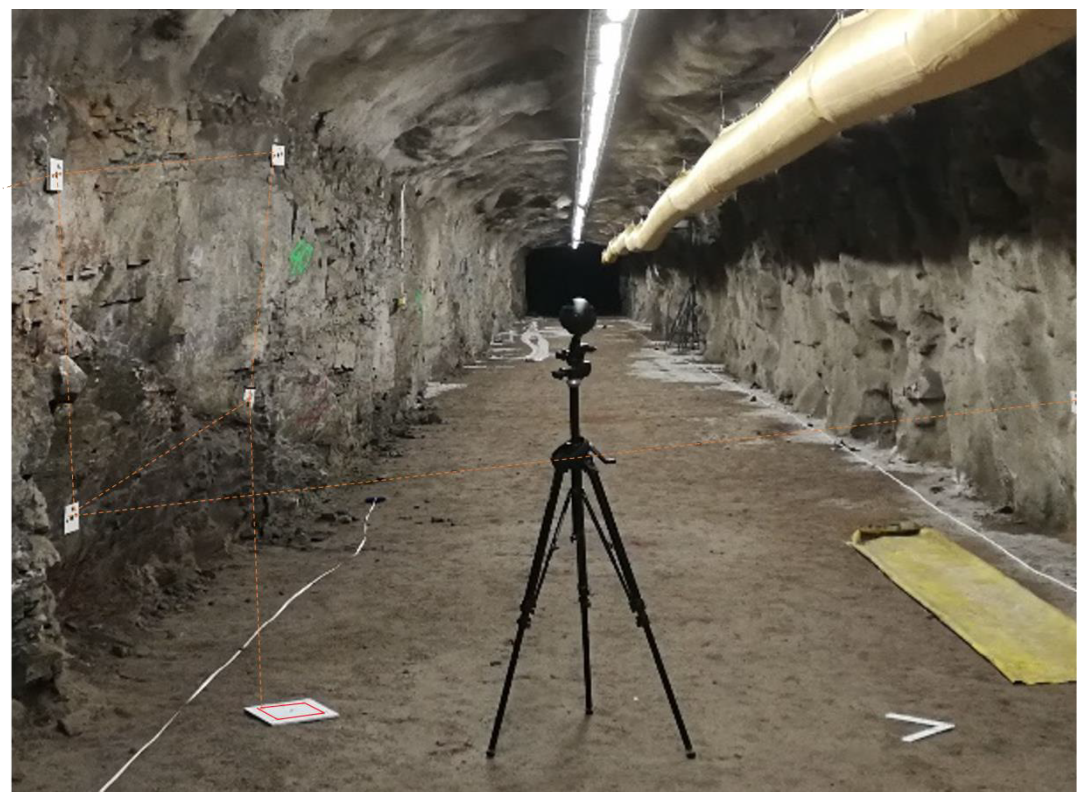
The Underground Research Laboratory of Aalto University (URLA) was selected as the test site for this study. URLA is located approximately 20 m below the Otaniemi campus in Espoo, Finland, and is used for field testing, research, and teaching activities [17]. The rock mass is composed of fine-grained hornblende-biotite gneiss and migmatic granite rocks and is moderately fractured with three main joint sets (two sub-vertical and one sub-horizontal set). The tunnel air temperature is approximately 14 °C, and the humidity is controlled with a fan and drying unit. The tunnel is illuminated with fluorescent lights installed on the roof (Figure 1) so portable lights are not required. The lighting remained constant during the testing of different cameras and image-capturing methods. This helps to have more control over the process.
A 10 m long tunnel section of a long mapping tunnel with a 5 m width and 3.5 m height was selected for this study. One wall of the tunnel is unsupported, and the rock is exposed, which makes it perfect for testing new methods to collect rock mass properties with remote mapping methods.
2.2. Control Points and Control Distances
To scale and rotate the model, an orientation control board (Figure 2a) was developed based on a similar tool developed in [3]. The board consists of five control points with a known distance between each point. The board is placed in the scanned scene and is aligned using a geological compass so that all the points lie on a horizontal plane and the arrow points in the North direction. This allows the 3D model to be properly rotated in space so that the orientation of rock mass discontinuities can be measured, especially when there are no ground control points available with known coordinates.
In addition, to measure the accuracy of the 3D model, 12 circular 20-bit control points (Figure 2b) were mounted on tunnel walls (6 points on the left wall and 6 on the right wall), and 26 distances between the points were measured with a Leica s910 laser distance meter. The points were then automatically detected by the photogrammetric software, and the calculated distances were compared with measured values (Figure 1) using the root-mean-square error (RMSE). The RMSE formula is presented in Equation (1).
where Pi is the measured value, Oi is the calculated value, and n is the number of measurements.
2.3. Image Acquisition with a 360-Degree Camera
A high-resolution 360-degree camera–Insta360 Pro–was used to scan the tunnel section (Figure 3a and Figure 1). The camera has a sensor of dimensions 6.311 × 4.721 mm and 4000 × 3000 pixel resolution. The camera has six fisheye 2 mm f/2.4 lenses so that six photos are captured each time, which are usually combined into a single equirectangular panorama. However, in this study, the raw 12 MPix resolution images from each lens were used instead (Figure 4b).
The camera was mounted on a tripod to allow for longer exposure times and photos were captured at 27 locations regularly spaced in two rows (Figure 4a), which resulted in 162 images. More camera locations were designed on the left side of the tunnel to increase the resolution of the exposed rock surface.
The images were captured with ISO set to 100 and a shutter speed of 1/7 s. The images were captured in RAW file format. The time to capture the photos was noted down and compared with the conventional workflow described in [17].
Next, the raw images were post-processed in Adobe Lightroom v10.4 to improve the visual quality of the textures applied to the reconstructed 3D models. The processing aimed to delight the images by decreasing the brightness of overexposed pixels and increasing brightness in shadows and improving sharpness by using the sharpening technique proposed by [26]. Post-processing settings are given in Table 1, and an example of the image postprocessing effect on a zoomed-in portion of the image can be seen in Figure 5. Note the improved visibility in darker areas and the improved sharpness throughout the image. The processed images were exported in .jpeg format and used for further processing in the photogrammetry software.
2.4. Photogrammetric Reconstruction
In this study, RealityCapture v.1.2 photogrammetric software [27] was chosen due to its fast reconstruction speed, reliability, and the authors’ previous experience. The reconstruction was done on a PC with an Intel i9-9900K @3.60 GHz CPU, 64 GB RAM, and an NVIDIA TITAN RTX GPU with 24 GB VRAM memory.
The processed images were imported into the software and the 3D models were reconstructed using the complete SfM-MVS workflow presented in [7]. First, the control points were detected automatically from each image. Next, all control points mounted on tunnel walls were temporarily disabled during alignment so that they did not influence the alignment. Next, the coordinates of the control points on the orientation board (Figure 2a) were set so that the bottom left corner of the board is located at the origin of a local Euclidean coordinate system (0,0,0) and other points lie on the same horizontal plane. The model was then aligned using the ‘K + Brown 4 with tangential2’ distortion model. The alignment settings are given in Table 2. The tie points were identified on all images and matched between the overlapping images. The camera locations were estimated, and a sparse point cloud was calculated.
Next, the dense point cloud was reconstructed using the MVS algorithm by projecting all identified points from 2D images to a 3D point cloud. The reconstruction was run on ‘High’ settings in the photogrammetric software, with an image downscale factor for depth maps set to 1. The mesh model was calculated from the point cloud. Finally, the model was textured with a maximal texture count unwrapping style and a maximum texture limit set to 6 textures of 8192 × 8192 pixels size. The model was then cropped and exported as a point cloud in .xyz format. The final steps were to enable all control points in the model, export the calculated control distances, and compute the average control distance, which was compared to the control distance measurements described in Section 2.2.
2.5. Reference Models
To test the quality of the 360-degree camera-based model, it was compared against three reference models: a laser scan and two photogrammetric models. The reference point clouds were placed in the same local coordinate system as the 360-camera-based model using the control points mounted on the tunnel wall. This enables direct comparison between the clouds.
The first model was a reference laser scan that was captured in the tunnel with a Riegl VZ-400i TLS scanner (Figure 3d) on the highest quality settings at six scanning stations (Figure 4a). The reference point cloud obtained with the laser scanner had a resolution of 0.005 m.
The second model was reconstructed with SfM-MVS from images captured with a Canon EOS RP Mirrorless DSLR camera with a full-frame sensor size of 36 × 24 mm (referred to as ‘DSLR’ going forward) equipped with a Canon EF 14 mm f/2.8L II USM lens (Figure 3b). The workflow for capturing the images of the entire tunnel section presented in [17] was used. In total, 111 images of 26.2 Mpix resolution were captured. The same alignment parameters as presented in Table 2 and reconstruction steps in the photogrammetric software were used.
The third model was reconstructed from the same 360-degree camera images as in the 360-degree camera-based model and additional high-resolution (HQ) images of the exposed rock wall captured with a DSLR camera. The assumption was that the resolution and visual quality of the 360-degree camera-based model can be improved considerably while keeping the capture time short. By adding additional high-resolution images captured in a relatively short time, the total capture time stays much shorter than the conventional method presented in [17] but the model achieves much better visual quality. The improved visual quality is especially important if the model will be used for rock mass characterization, in which some parameters of the rock are assessed visually [28], or if the model will be used for VR/AR-based rock mass mapping systems [28,29,30,31,32]. For this purpose, 13 high-resolution images of the unsupported tunnel wall were captured (Figure 4a) with a Canon 5Ds R full-frame DSLR camera and Canon EF 35 mm f/1.4 L II USM prime lens (Figure 3c).
However, it should be noted that the data for the reference models were collected later than the 360-degree image acquisition due to the unavailability of the hardware. This resulted in small changes in the geometry of the site; for example, the position of the ventilation tubing had changed, and minor rock pieces were spotted on the tunnel floor. Therefore, part of the floor of the tunnel and the ventilation tubing were cropped out of all the point clouds.
2.6. Point Cloud Data Analysis
The 3D point clouds were processed in Cloud Compare v2.12.0 software [33]. First, the clouds were cleaned by removing outliers using the ‘Statistical Outlier Removal’ function with six points used for mean distance estimates and a standard deviation multiplier threshold of 1.
Next, the surface density of the clouds was calculated with the ‘Compute geometric features’ function and a local neighborhood radius of 0.005 m. The point density of the entire tunnel section and the exposed rock wall was examined and compared with the reference models.
Finally, the 360-degree camera and the other two photogrammetrically obtained reference point clouds were compared against the TLS scan to measure the accuracy of photogrammetric reconstruction. For this purpose, the ‘Cloud-to-Cloud (C2C)’ distance function was used, and distances were computed and analyzed.
2.7. Remote Rock Mass Measurements
To test the quality of the remote rock mass measurements obtained from the 3D models of the scanned tunnel section, the point clouds of the exposed rock wall were analyzed using the Discontinuity Set Extractor (DSE) software [5]. DSE software clusters the points into planes of similar orientation and allows a semi-automatic rock mass discontinuity mapping. The mean orientation of the extracted discontinuity sets obtained with the DSE software was compared with manual compass measurements obtained in a previous study [30].
3. Results and Discussion
3.1. Image Acquisition Time and Photogrammetric Reconstruction
The process described in Section 2, above, resulted in the production of high-resolution colored point clouds of the tunnel section (Figure 6, Figure 7 and Figure 8). The time to capture the photos and the resulting model quality was compared against the conventional DSLR camera and workflow described in [17]. Capturing the images of the same tunnel section with the 360-degree camera took only 10 min compared to the 34 min for capturing 111 images with a DSLR camera (see Table 3).
Even though the quality of the 360-degree camera-based model was visually acceptable and comparable to the reference DSLR model (Figure 7a,b), the surface density of the point cloud was slightly lower than the DSLR model, and the points were not evenly distributed on the tunnel wall (Figure 7a). This was most likely the result of the smaller sensor size, lower pixel resolution and focal length of the 360-degree camera, and an uneven overlap on the tunnel wall due to the slight rotation of the camera when moving between the camera locations.
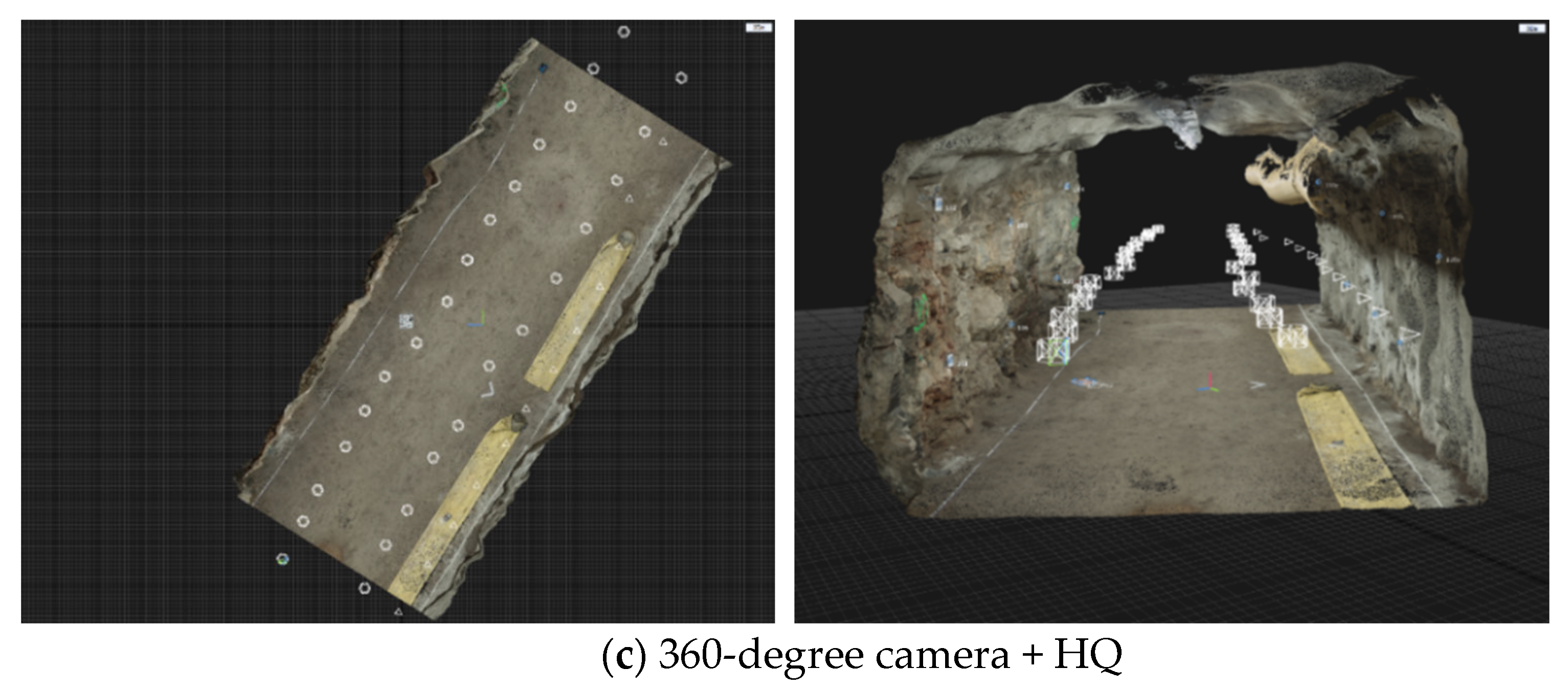
The improved model utilizing both 360-degree and HQ images is presented in Figure 6c. The improved model achieves almost 4× higher point density (see Table 3 and Figure 7c) while the capture time is only 4 min longer and the overall processing time is only 11 min longer. In addition, the point density is more evenly distributed on the tunnel wall (Figure 7c and Figure 8c). The combined 360-degree and HQ model achieves comparable results to the model created with only DSLR images (Figure 7b), but the image capturing time and processing time is much faster, and the point density of the tunnel wall is higher (Figure 8c).
The fast image acquisition speed, acceptable point density, and low processing time obtained in this study confirm that 360-degree cameras can be successfully used for the photogrammetric digitization of tunnels. The 360-degree model achieves comparable results to a conventional DSLR camera, and the workflow is less prone to mistakes.
The K + Brown4 with tangential2 distortion model that was used for alignment of the 3D model in this study resulted in a more accurate alignment compared to the K + Brown3 distortion model used in the previous test [25]. The mean projection error has dropped to 0.296 pixels from the previously achieved 0.482 pixels.
3.2. Control Distance Error and Comparison with a Reference Model
The accuracy of the scan was first tested by physically measuring distances between control points attached to the walls of the tunnel (Figure 9 and Figure 10) as described in Section 2.2. Distances measured with the physical tool were taken as control distances. The measured and calculated distances and the corresponding RMSE value calculated for each model are presented in Table 4. The RMSE of each model was calculated according to Equation (1).
The RMSE of the control distances amounted to 0.0082 m for the 360-degree camera-based model. In comparison, the DSLR model achieved an RMSE of 0.0099 m, and the improved 360 + HQ model was 0.0095 m. The RMSE of the control distances measured on the reference TLS scan amounted to 0.0090 m. The resulting control distance accuracy of the 360-degree camera-based model can be considered acceptable for the given tunnel dimensions and measurement method. It should also be noted that the laser distance measurement device that was used for control distance measurements has an accuracy of ±1 mm. The lower accuracy of the TLS can be attributed to the measurement technique. The control points in the TLS model were detected and measured manually in Cloud Compare software, whereas all control points in the photogrammetric models were detected automatically and the distances were also measured automatically.
Next, the difference between the reference TLS scan and the photogrammetric models was tested by computing the Cloud-to-cloud (C2C) distance between the point clouds. The 360-degree camera-based model achieved a 0.0046 m Root Mean Square (RMS) C2C difference from the reference laser scan. The RMS value was computed from all scalar values at each point. In comparison, the conventional DSLR model achieved a 0.0050 m difference, and the improved 360 + HQ model achieved a 0.0043 m difference (Table 5). In addition, to limit the effect of outliers, a Gauss distribution was fitted to the C2C results for each model, and the mean value, and the upper and lower limit of C2C computed as two standard deviations, are presented in Table 5. It can be observed that the C2C error is lower compared to the C2C obtained using the RMS of all points and the mean C2C of the 360-degree model ranges up to 0.0088 m with 95% confidence.
The C2C results for each point cloud of the tunnel section are presented in Figure 11 with the color scale ranging from 0 to 0.02 m. In addition, the histogram of the C2C results can be seen on the right side of the color scale. The largest C2C distances on the 360-degree and 360-degree + HQ clouds were measured on the small rock pieces on the left side of the tunnel floor (red colored points in Figure 11a,c). This was because the reference DSLR and TLS scans were made later than the 360-degree image acquisition and some minor tunnel geometry changes took place, mainly due to small rock pieces detaching from the tunnel wall or roof and landing on the floor. This means that the mean C2C distances presented in this study can be considered conservative, and a smaller distance to the TLS scan could be achieved if the scans took place simultaneously.
It was also observed that in the improved model with additional high-quality images of the tunnel wall, the accuracy has increased. This can be seen in Figure 11c, in which the left tunnel wall has a reduced C2C compared to the model with only 360-degree images (Figure 11a).
In overall, the accuracy of the 360-degree camera scan can be considered as good and acceptable for rapid tunnel digitization with the SfM-MVS method, where speed should sometimes be favored over accuracy [34]. The accuracy achieved with the settings used in this study is comparable to the previous study where 360-degree cameras were used to create 3D models with SfM-MVS photogrammetry [21]. The high accuracy can be attributed to the high-quality camera used in this study, which was also predicted by Barazetti et al. in [21]. In comparison, if a low-cost spherical camera is used (e.g., [24]) C2C distances up to 15 cm and noisy clouds without fine details reconstructed can be expected.
3.3. Rock Mass Characterization
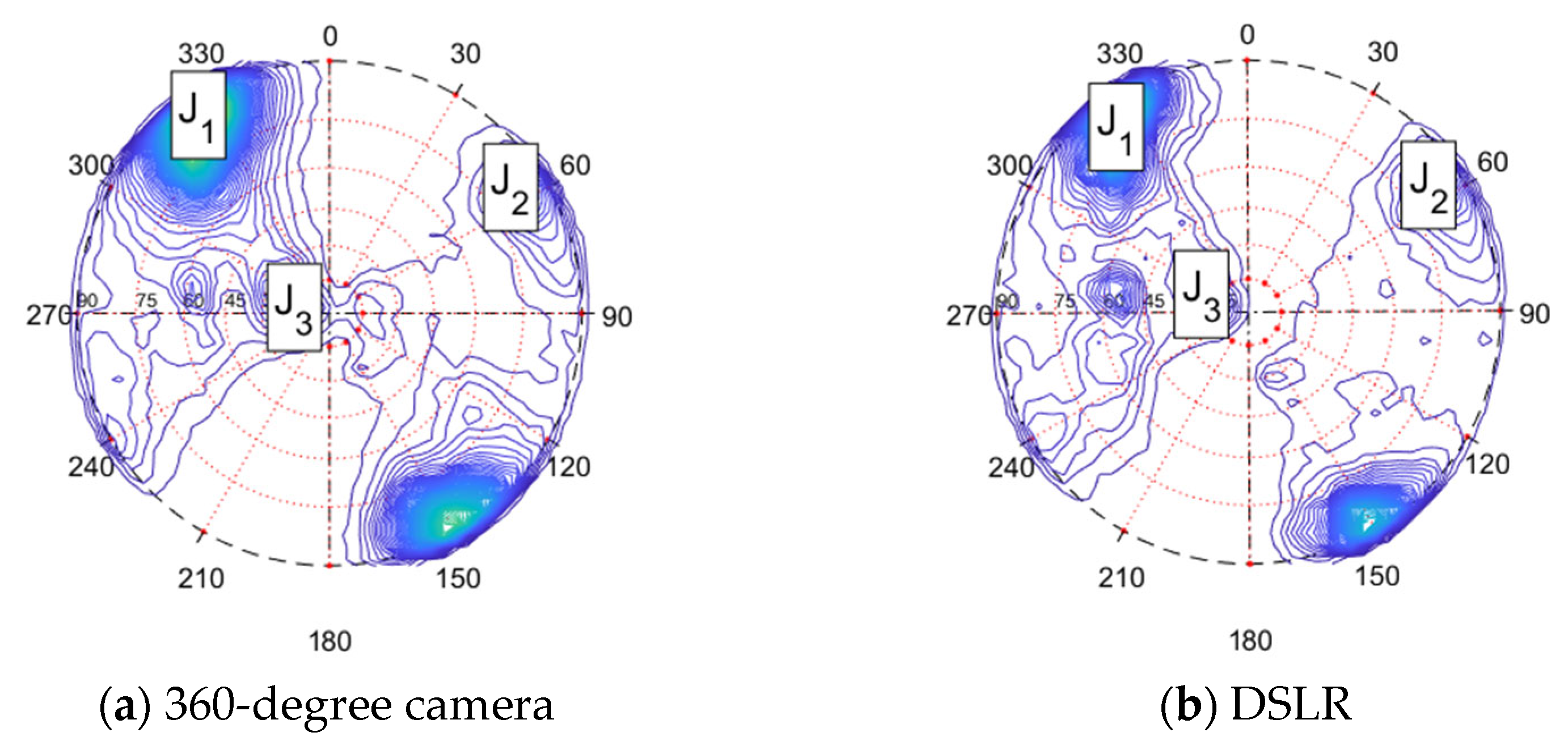
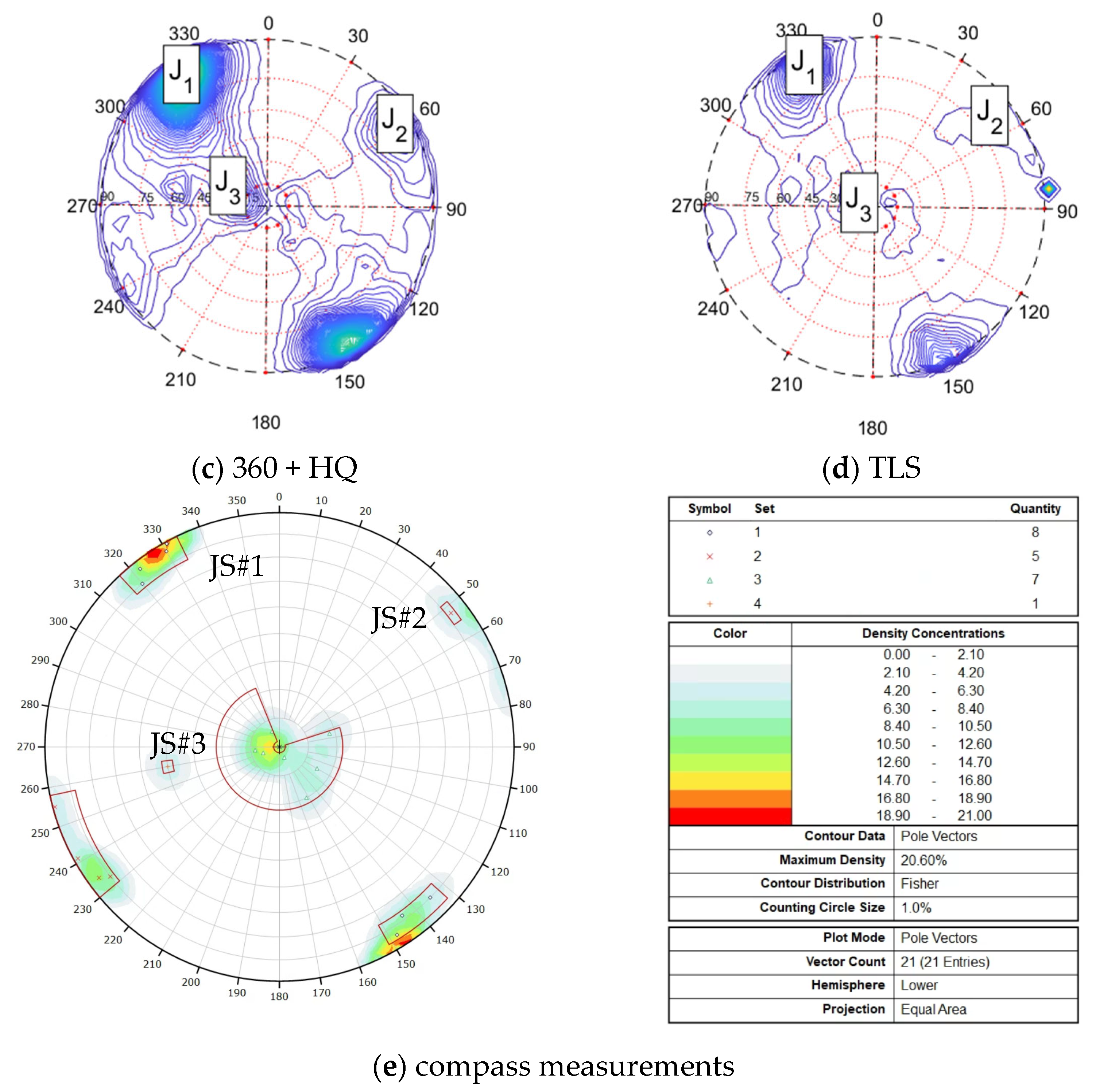
Next, the remote mapping of rock mass properties was tested on the given 3D models of the tunnel wall. The point clouds were cropped to a 2 × 1.3 m mapping window (Figure 12) that was previously mapped with a conventional geological compass [17,30]. Discontinuity sets and their geometrical properties were extracted from the 3D models using the semi-automatic automatic method in the Discontinuity Set Extractor software [5]. The data was processed, three main joint sets were identified in all three models and their mean orientation was extracted. The results of the remote mapping are presented in Figure 12, Figure 13 and Table 6.
The computed mean orientation (dip direction and dip) of the extracted rock mass discontinuity planes from the three photogrammetrically-obtained point clouds and the TLS scan agrees well with 21 measurements obtained in previous studies [17,30] using a conventional geological compass (see Table 6 and Figure 13). The reference TLS scan obtains the most accurate dip direction and dip measurement of the identified fracture planes. The 360-degree camera-based model achieves comparable results that are also consistent with the reference DSLR model. The addition of high-quality images of the rock surface does not increase the accuracy of remote measurements considerably. However, the accuracy of the dip measurement of joint set 3 was improved in this experiment.
The differences between the remote and conventional measurements of fracture orientation are the lowest for the two sub-vertical planes (joint sets 1 and 2). However, the orientation of the sub-horizontal plane is not accurately measured. This is a common issue attributed mainly to a lower amount of light on such a plane and the low angle between the camera and the horizontal surface affecting the line of sight. Similar observations were made in [35], where rock mass measurements obtained from mobile laser scanning were generally accurate, but the sub-horizontal fracture set was not detected and required additional scanning rounds. It should be noted that field mapping with a conventional geological compass can also vary by a few degrees, which is affected by human bias and the quality of the compass. This is especially visible when mapping sub-horizontal features [18]. Therefore, the remote rock mass mapping result of this study can be considered successful since it was possible to detect all joint sets, including the sub-horizontal planes but with lower accuracy compared to more favorably oriented discontinuity planes. The accuracy of the remote mapping can be improved by including additional images taken from lower and higher positions relative to the horizontal fracture planes so that the point density in the shadow areas would be increased and more data points would be used to extract the planes and compute the orientation [18].
4. Conclusions
This study presented a complete workflow for underground tunnel digitization using a 360-degree camera and Structure-from-Motion Multi-View Stereo photogrammetry. The method was tested on a 10 m-long hard rock tunnel section. The results demonstrate that a 360-degree camera is a viable instrument to rapidly capture high-quality data for the photogrammetric reconstruction of underground tunnels. The image acquisition time amounted to 10 min per 10 m long tunnel section and was one-third compared to that of a conventional camera. The reconstructed 3D model achieved 0.0046 m distance accuracy when compared to a reference laser scan, and 21 pts/cm2 point cloud resolution.
The 360-camera-based model was also used to remotely map rock mass properties. The mean orientation of three identified discontinuity sets was measured using a semi-automatic method. The results matched the field measurements obtained using a conventional geological compass for the two sub-vertical sets with an average error of 2–5°, although some discrepancies were observed for sub-horizontal planes, which is a common issue reported in the literature.
The resolution and accuracy of the 360-degree camera-based model were improved by capturing additional high-resolution images of the mapped tunnel. The improved model achieved 97 pts/cm2 point resolution of the tunnel wall while increasing the total capture time to only 14 min. The improved resolution is beneficial if small features must be mapped for rock mass characterization purposes.
As a next step, for practical validation, it is recommended to test the same equipment in more challenging tunnel conditions resembling an ongoing excavation process with high dust and moisture content in the air.
Author Contributions
Conceptualization, M.J.; methodology, M.J.; data collection, M.J and M.T.; data analysis, M.J. and M.T.; writing—original draft preparation, M.J.; writing—review and editing, M.T., L.U., M.R.; visualization, M.J.; supervision, M.R.; project administration, M.R., L.U. and M.J.; funding acquisition, M.J. and L.U. All authors have read and agreed to the published version of the manuscript.
Funding
This research was funded by the Academy of Finland, grant number 319798. The authors greatly appreciate the financial support.
Data Availability Statement
Not applicable.
Acknowledgments
This research was part of the GAGS project. The authors greatly appreciate the financial support.
Conflicts of Interest
The authors declare no conflict of interest. The funders had no role in the design of the study; in the collection, analyses, or interpretation of data; in the writing of the manuscript, or in the decision to publish the results.
References
- Attard, L.; Debono, C.J.; Valentino, G.; Di Castro, M. Tunnel inspection using photogrammetric techniques and image processing: A review. ISPRS J. Photogramm. Remote Sens. 2018, 144, 180–188. [Google Scholar] [CrossRef]
- Hudson, J.; Harrison, J. Engineering Rock Mechanics: An Introduction to the Principles, 2nd ed.; Elsevier: Oxford, UK, 2000. [Google Scholar]
- García-Luna, R.; Senent, S.; Jurado-Piña, R.; Jimenez, R. Structure from Motion photogrammetry to characterize underground rock masses: Experiences from two real tunnels. Tunn. Undergr. Space Technol. 2019, 83, 262–273. [Google Scholar] [CrossRef]
- Uotinen, L.; Janiszewski, M.; Baghbanan, A.; Caballero Hernandez, E.; Oraskari, J.; Munukka, H.; Szydlowska, M.; Rinne, M. Photogrammetry for recording rock surface geometry and fracture characterization. In Proceedings of the Earth and Geosciences, the 14th International Congress on Rock Mechanics and Rock Engineering (ISRM 2019), Foz do Iguassu, Brazil, 13–18 September 2019; da Fontoura, S.A.B., Rocca, R.J., Pavón Mendoza, J.F., Eds.; CRC Press: Boca Raton, FL, USA, 2019; Volume 6, pp. 461–468. [Google Scholar]
- Riquelme, A.J.; Abellán, A.; Tomás, R.; Jaboyedoff, M. A new approach for semi-automatic rock mass joints recognition from 3D point clouds. Comput. Geosci. 2014, 68, 38–52. [Google Scholar] [CrossRef] [Green Version]
- Ding, Q.; Wang, F.; Chen, J.; Wang, M.; Zhang, X. Research on Generalized RQD of Rock Mass Based on 3D Slope Model Established by Digital Close-Range Photogrammetry. Remote Sens. 2022, 14, 2275. [Google Scholar] [CrossRef]
- Torkan, M.; Janiszewski, M.; Uotinen, L.; Baghbanan, A.; Rinne, M. Photogrammetric Method to Determine Physical Aperture and Roughness of a Rock Fracture. Sensors 2022, 22, 4165. [Google Scholar] [CrossRef]
- Panella, F.; Roecklinger, N.; Vojnovic, L.; Loo, Y.; Boehm, J. Cost-benefit analysis of rail tunnel inspection for photogrammetry and laser scanning. ISPRS—Int. Arch. Photogramm. Remote Sens. Spat. Inf. Sci. 2020, XLIII-B2-2020, 1137–1144. [Google Scholar] [CrossRef]
- Fekete, S.; Diederichs, M.; Lato, M. Geotechnical and operational applications for 3-dimensional laser scanning in drill and blast tunnels. Tunn. Undergr. Space Technol. 2010, 25, 614–628. [Google Scholar] [CrossRef]
- Cawood, A.J.; Bond, C.E.; Howell, J.A.; Butler, R.W.H.; Totake, Y. LiDAR, UAV or compass-clinometer? Accuracy, coverage and the effects on structural models. J. Struct. Geol. 2017, 98, 67–82. [Google Scholar] [CrossRef]
- Francioni, M.; Simone, M.; Stead, D.; Sciarra, N.; Mataloni, G.; Calamita, F. A New Fast and Low-Cost Photogrammetry Method for the Engineering Characterization of Rock Slopes. Remote Sens. 2019, 11, 1267. [Google Scholar] [CrossRef] [Green Version]
- Ulman, S. The interpretation of structure from motion. Proc. R. Soc. Lond. B. Biol Sci. 1979, 203, 405–426. [Google Scholar]
- Lowe, D.G. Distinctive image features from Scale-Invariant Keypoints. Int. J. Comput. Vis. 2004, 60, 91–110. [Google Scholar] [CrossRef]
- Snavely, N.; Seitz, S.M.; Szeliski, R. Photo tourism: Exploring photo collections in 3D. ACM Trans. Graph. 2006, 25, 835–846. [Google Scholar] [CrossRef] [Green Version]
- Furukawa, Y.; Hernández, C. Multi-View Stereo: A Tutorial. Found. Trends Comput. Graph. Vis. 2015, 9, 1–148. [Google Scholar] [CrossRef] [Green Version]
- Westoby, M.J.; Brasington, J.; Glasser, N.F.; Hambrey, M.J.; Reynolds, J.M. ‘Structure-from-Motion’ photogrammetry: A low-cost, effective tool for geoscience applications. Geomorphology 2012, 179, 300–314. [Google Scholar] [CrossRef] [Green Version]
- Janiszewski, M.; Uotinen, L.; Baghbanan, A.; Rinne, M. Digitisation of hard rock tunnel for remote fracture mapping and virtual training environment. In Proceedings of the ISRM International Symposium—EUROCK 2020, Trondheim, Norway, 14–19 June 2020. Physical Event Not Held, ISRM-EUROCK-2020-056. [Google Scholar]
- Prittinen, M. Comparison of Camera Equipment for Photogrammetric Digitization of Hard Rock Tunnel Faces. Master’s Thesis, Aalto University, Espoo, Finland, 2021. [Google Scholar]
- Perfetti, L.; Polari, C.; Fassi, F. Fisheye photogrammetry: Tests and methodologies for the survey of narrow spaces. Int. Arch. Photogramm. Remote Sens. Spatial Inf. Sci. 2017, XLII-2/W3, 573–580. [Google Scholar] [CrossRef] [Green Version]
- Fangi, G.; Pierdicca, R.; Sturari, M.; Malinverni, E.S. Improving spherical photogrammetry using 360° omni-cameras: Use cases and new applications. Int. Arch. Photogramm. Remote Sens. Spatial Inf. Sci. 2018, XLII-2, 331–337. [Google Scholar] [CrossRef] [Green Version]
- Barazzetti, L.; Previtali, M.; Roncoroni, F. 2018 Can we use low-cost 360-degree cameras to create accurate 3d models? Int. Arch. Photogramm. Remote Sens. Spatial Inf. Sci. 2018, XLII-2, 69–75. [Google Scholar] [CrossRef] [Green Version]
- Barazzetti, L.; Previtali, M.; Scaioni, M. Procedures for Condition Mapping Using 360° Images. ISPRS Int. J. Geo-Inf. 2020, 9, 34. [Google Scholar] [CrossRef] [Green Version]
- Teppati Losè, L.; Chiabrando, F.; Giulio Tonolo, F. Documentation of Complex Environments Using 360° Cameras. The Santa Marta Belltower in Montanaro. Remote Sens. 2021, 13, 3633. [Google Scholar] [CrossRef]
- Herban, S.; Costantino, D.; Alfio, V.S.; Pepe, M. Use of Low-Cost Spherical Cameras for the Digitisation of Cultural Heritage Structures into 3D Point Clouds. J. Imaging 2022, 8, 13. [Google Scholar] [CrossRef]
- Janiszewski, M.; Prittinen, M.; Torkan, M.; Uotinen, L. Rapid tunnel scanning using a 360-degree camera and SfM photogrammetry. In Proceedings of the EUROCK 2022, Espoo, Finland, 12–15 September 2022. accepted. [Google Scholar]
- Cox, H. Advanced Post-Processing Tips: Three-Step Sharpening. 2016. Available online: https://photographylife.com/landscapes/advanced-post-processing-tips-three-step-sharpening (accessed on 17 August 2022).
- RealityCapture, Version 1.2, by CapturingReality. Available online: www.capturingreality.com (accessed on 15 August 2022).
- Zhang, Y.; Yue, P.; Zhang, G.; Guan, T.; Lv, M.; Zhong, D. Augmented Reality Mapping of Rock Mass Discontinuities and Rockfall Susceptibility Based on Unmanned Aerial Vehicle Photogrammetry. Remote Sens. 2019, 11, 1311. [Google Scholar] [CrossRef]
- Janiszewski, M.; Uotinen, L.; Merkel, J.; Leveinen, J.; Rinne, M. Virtual reality Learning Environments for Rock Engineering, Geology and Mining Education. In Proceedings of the 54th U.S. Rock Mechanics/Geomechanics Symposium, Denver, CO, USA, 28 June–1 July 2020; ARMA-2020-1101. Available online: https://onepetro.org/ARMAUSRMS/proceedings-abstract/ARMA20/All-ARMA20/ARMA-2020-1101/447531 (accessed on 15 August 2022).
- Jastrzebski, J. Virtual Underground Training Environment. Master’s Thesis, Aalto University, Espoo, Finland, 2018. [Google Scholar]
- Zhang, X. A Gamifed Rock Engineering Teaching System. Master’s Thesis, Aalto University, Espoo, Finland, 2021. [Google Scholar]
- Janiszewski, M.; Uotinen, L.; Szydlowska, M.; Munukka, H.; Dong, J. Visualization of 3D rock mass properties in underground tunnels using extended reality. IOP Conf. Ser. Earth Environ. Sci. 2021, 703, 012046. [Google Scholar] [CrossRef]
- CloudCompare, Version 2.12.4. Available online: https://https://www.cloudcompare.org/ (accessed on 15 August 2022).
- Bauer, A.; Gutjahr, K.; Paar, G.; Kontrus, H.; Glatzl, R. Tunnel Surface 3D Reconstruction from Unoriented Image Sequences. In Proceedings of the OAGM Workshop 2015, 22 May 2015; Available online: https://arxiv.org/abs/1505.06237 (accessed on 15 August 2022).
- Eyre, M.; Wetherelt, A.; Coggan, J. Evaluation of automated underground mapping solutions for mining and civil engineering applications. J. Appl. Remote Sens. 2016, 10, 046011. [Google Scholar] [CrossRef]
Figure 1.
Photo depicting part of the tunnel section that was selected for testing the 360-degree camera for photogrammetric digitization and remote rock mass mapping. Control distances were measured between the control points mounted on the tunnel wall (example illustrated with an orange dashed line). An orientation board with four control points was placed on the floor (white board in the lower left corner) and was used to orient the model.

Figure 2.
Orientation control board (a) with known local coordinates used to orient the 3D model, and (b) control point example that was used in the field test to control the accuracy of SfM-MVS reconstruction.
Figure 2.
Orientation control board (a) with known local coordinates used to orient the 3D model, and (b) control point example that was used in the field test to control the accuracy of SfM-MVS reconstruction.
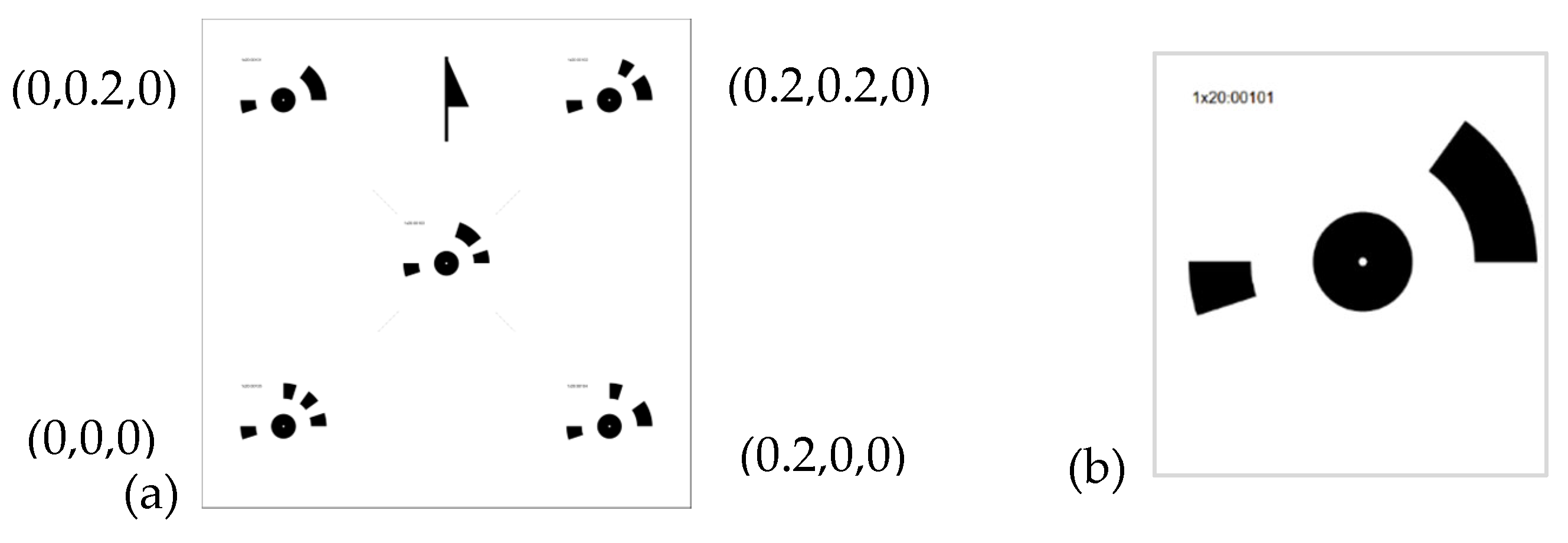
Figure 3.
Hardware used in this study: (a) Insta360 Pro with 6 fisheye lenses, (b) Canon EOS RP mirrorless DSLR with 14 mm lens to capture the reference DSLR model, (c) Canon 5Ds R DSLR with 35 mm lens to capture the High-Quality images for the improved 360 + HQ model, and (d) Riegl VZ-400i terrestrial laser scanner.

Figure 4.
Planned image network with 27 locations of the 360-degree camera at the test site of the Underground Research Laboratory of Aalto University (a), and the raw image from one of the six lenses in the 360-degree camera (b).
Figure 4.
Planned image network with 27 locations of the 360-degree camera at the test site of the Underground Research Laboratory of Aalto University (a), and the raw image from one of the six lenses in the 360-degree camera (b).

Figure 5.
Comparison of the raw (left) and processed (right) image that was delighted and sharpened in Adobe Lightroom; detailed settings used are given in Table 1.
Figure 5.
Comparison of the raw (left) and processed (right) image that was delighted and sharpened in Adobe Lightroom; detailed settings used are given in Table 1.
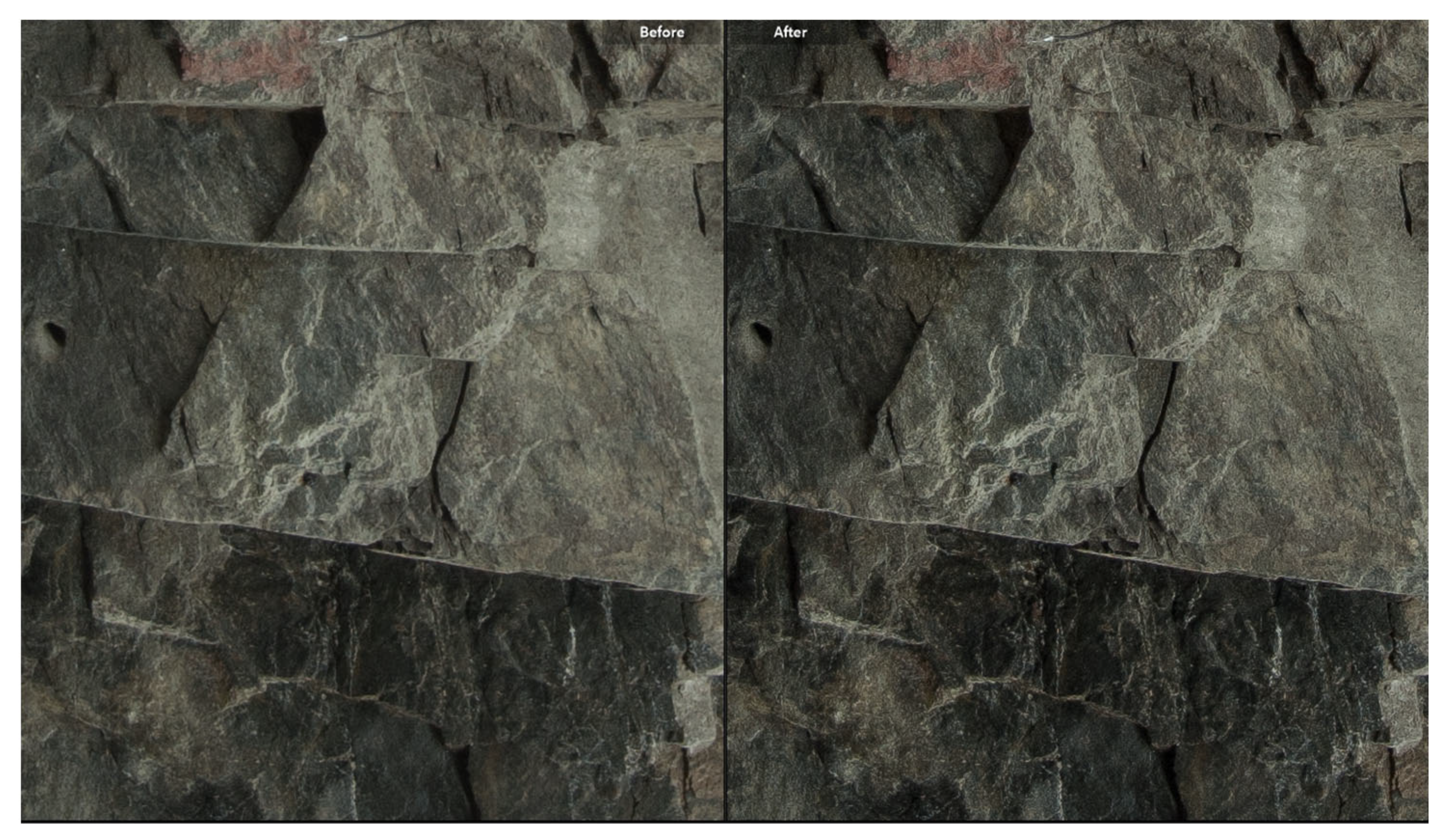
Figure 6.
Top view (left) and front view (right) of the scanned tunnel 3D model reconstructed with SfM-MVS photogrammetry from images captured using: (a) 360-degree camera, (b) DSLR camera, and (c) 360-degree camera and HQ images captured by a DSLR camera for improved resolution of the wall.
Figure 6.
Top view (left) and front view (right) of the scanned tunnel 3D model reconstructed with SfM-MVS photogrammetry from images captured using: (a) 360-degree camera, (b) DSLR camera, and (c) 360-degree camera and HQ images captured by a DSLR camera for improved resolution of the wall.


Figure 7.
3D point clouds and surface point density of the tunnel wall digitized with: (a) 360-degree camera-based photogrammetric model, (b) DSLR model for comparison, and (c) an improved model with additional DSLR images of the tunnel wall.
Figure 7.
3D point clouds and surface point density of the tunnel wall digitized with: (a) 360-degree camera-based photogrammetric model, (b) DSLR model for comparison, and (c) an improved model with additional DSLR images of the tunnel wall.
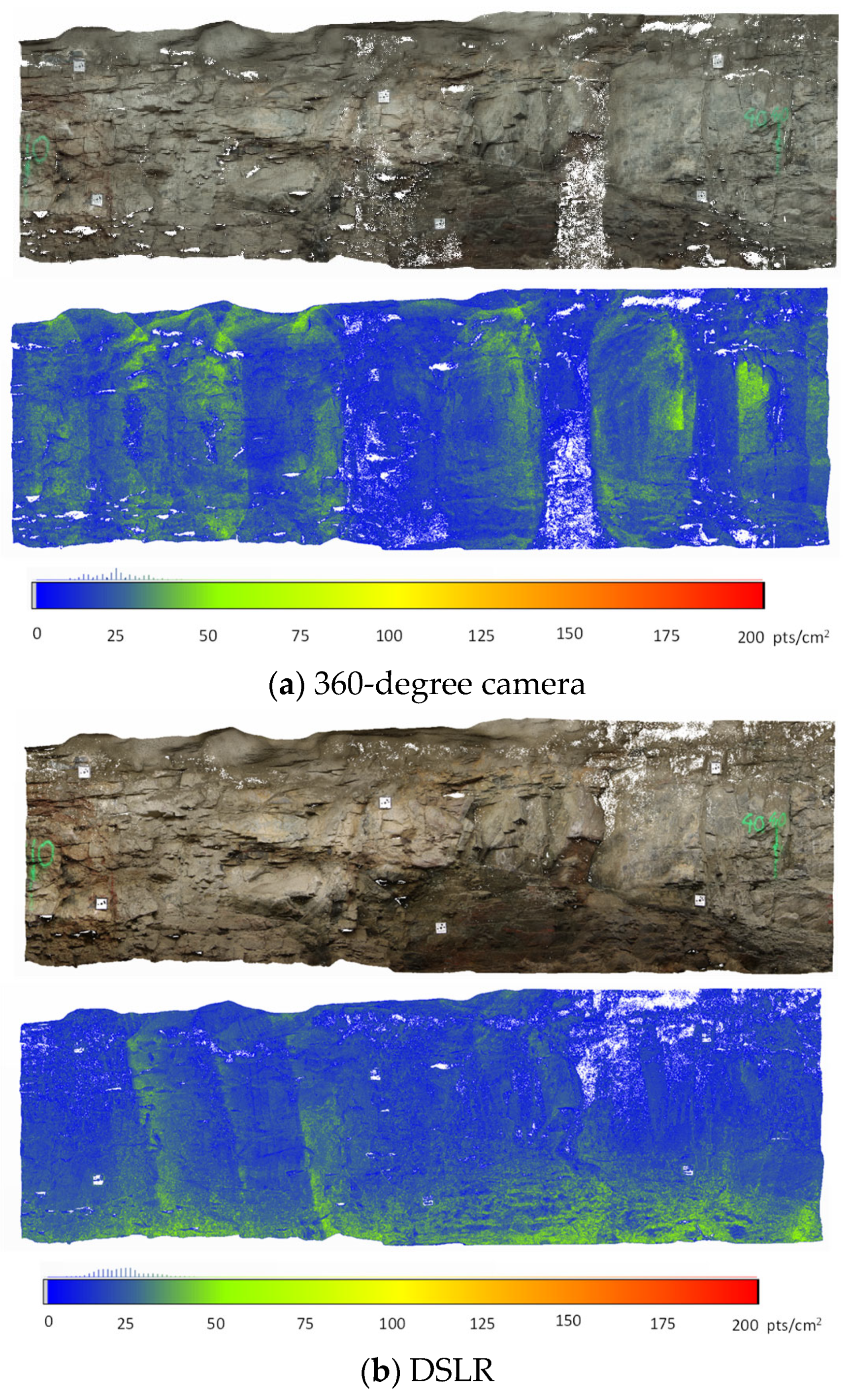
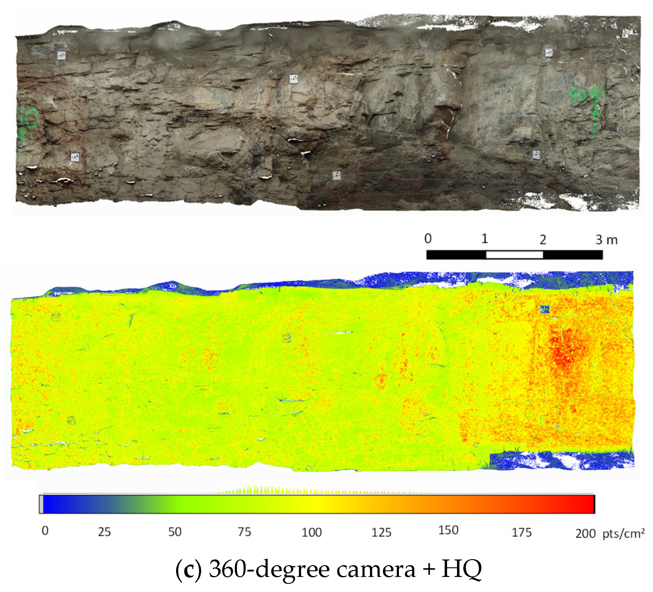
Figure 8.
Surface point density of the 3D point cloud of the entire tunnel section digitized with: (a) 360-degree camera, (b) DSLR, and (c) 360-degree camera with HQ images of the tunnel wall.
Figure 8.
Surface point density of the 3D point cloud of the entire tunnel section digitized with: (a) 360-degree camera, (b) DSLR, and (c) 360-degree camera with HQ images of the tunnel wall.
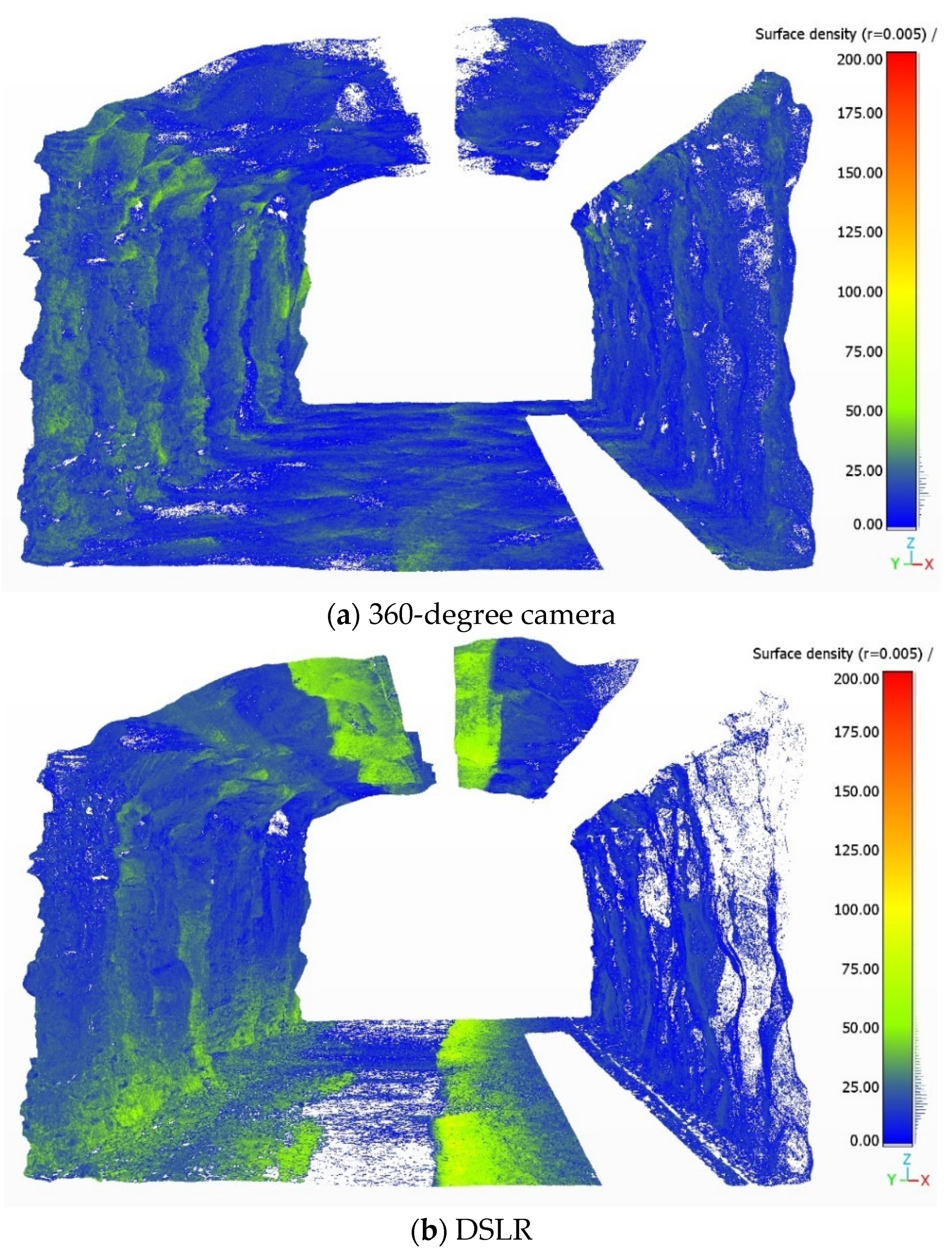

Figure 9.
Control distances were measured between markers mounted on tunnel walls and compared with the calculated distances on the reconstructed 3D model.
Figure 9.
Control distances were measured between markers mounted on tunnel walls and compared with the calculated distances on the reconstructed 3D model.
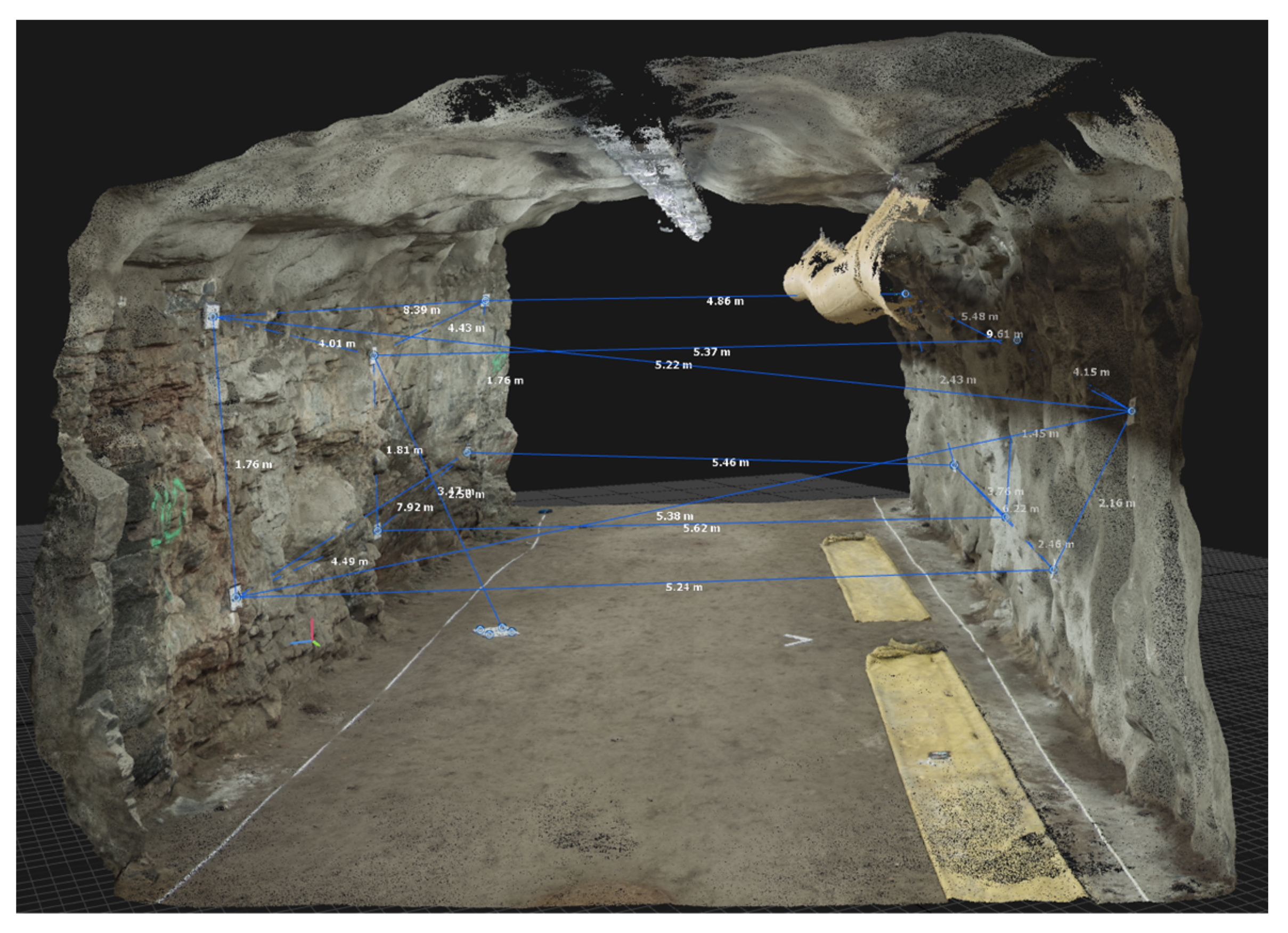
Figure 10.
Reference point cloud of the tunnel section (above) with a uniform point density (below), obtained with the Riegl VZ-400i terrestrial laser scanner (TLS).
Figure 10.
Reference point cloud of the tunnel section (above) with a uniform point density (below), obtained with the Riegl VZ-400i terrestrial laser scanner (TLS).
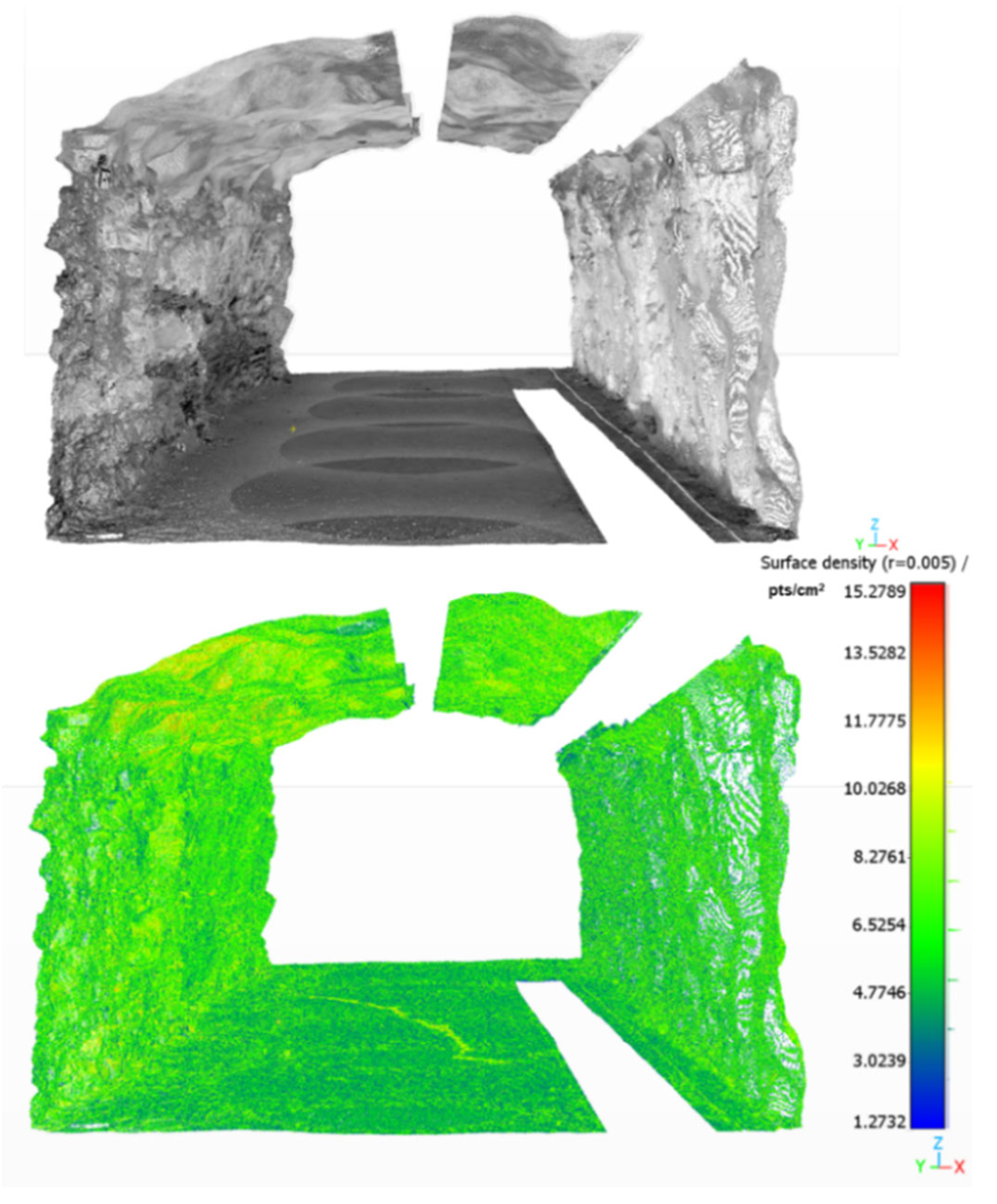
Figure 11.
Cloud-to-cloud (C2C) distance between the reference TLS laser scan and the 3D point cloud of the tunnel wall digitized with: (a) 360-degree camera, (b) DSLR, and (c) 360-degree camera with HQ images of the tunnel wall.
Figure 11.
Cloud-to-cloud (C2C) distance between the reference TLS laser scan and the 3D point cloud of the tunnel wall digitized with: (a) 360-degree camera, (b) DSLR, and (c) 360-degree camera with HQ images of the tunnel wall.
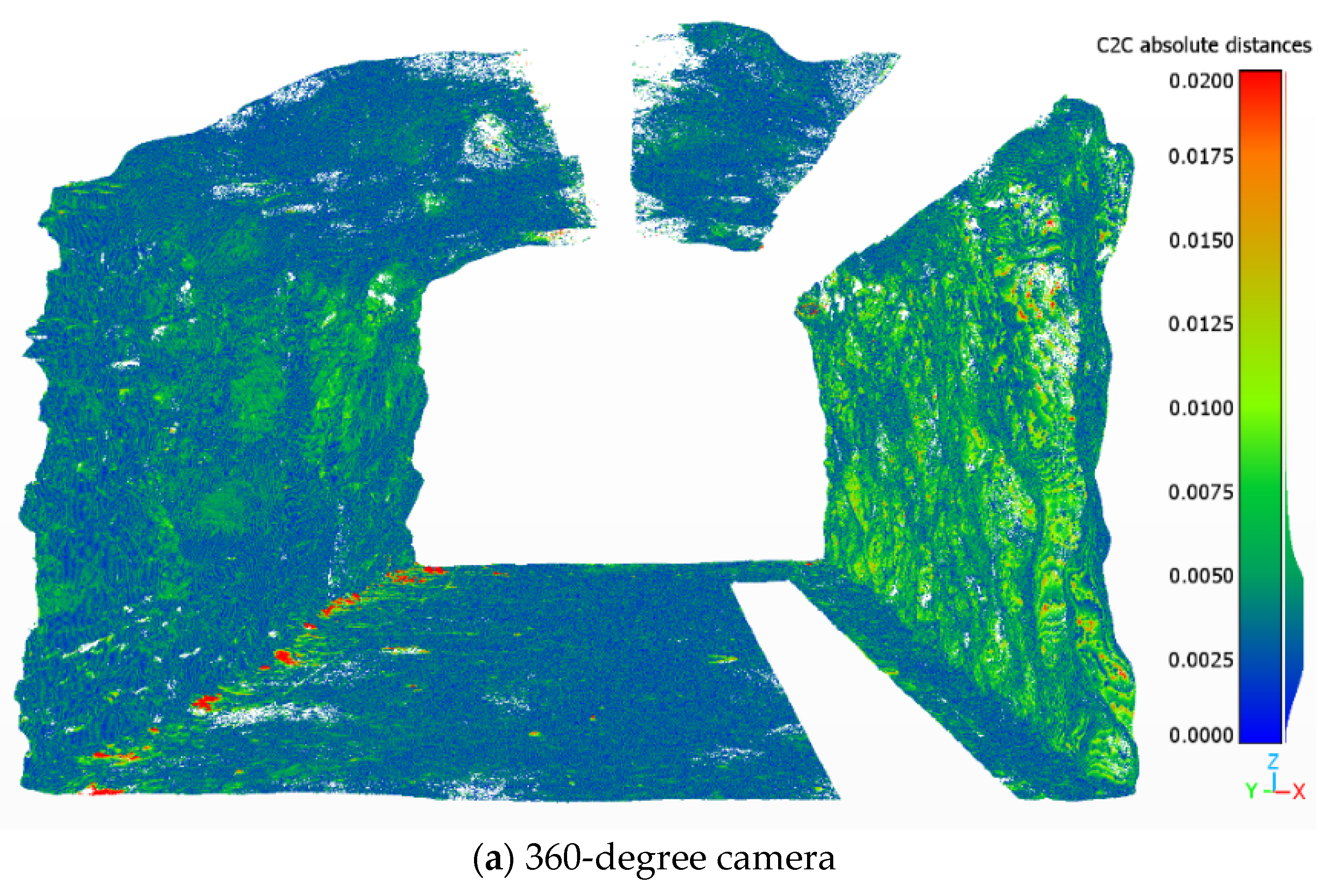
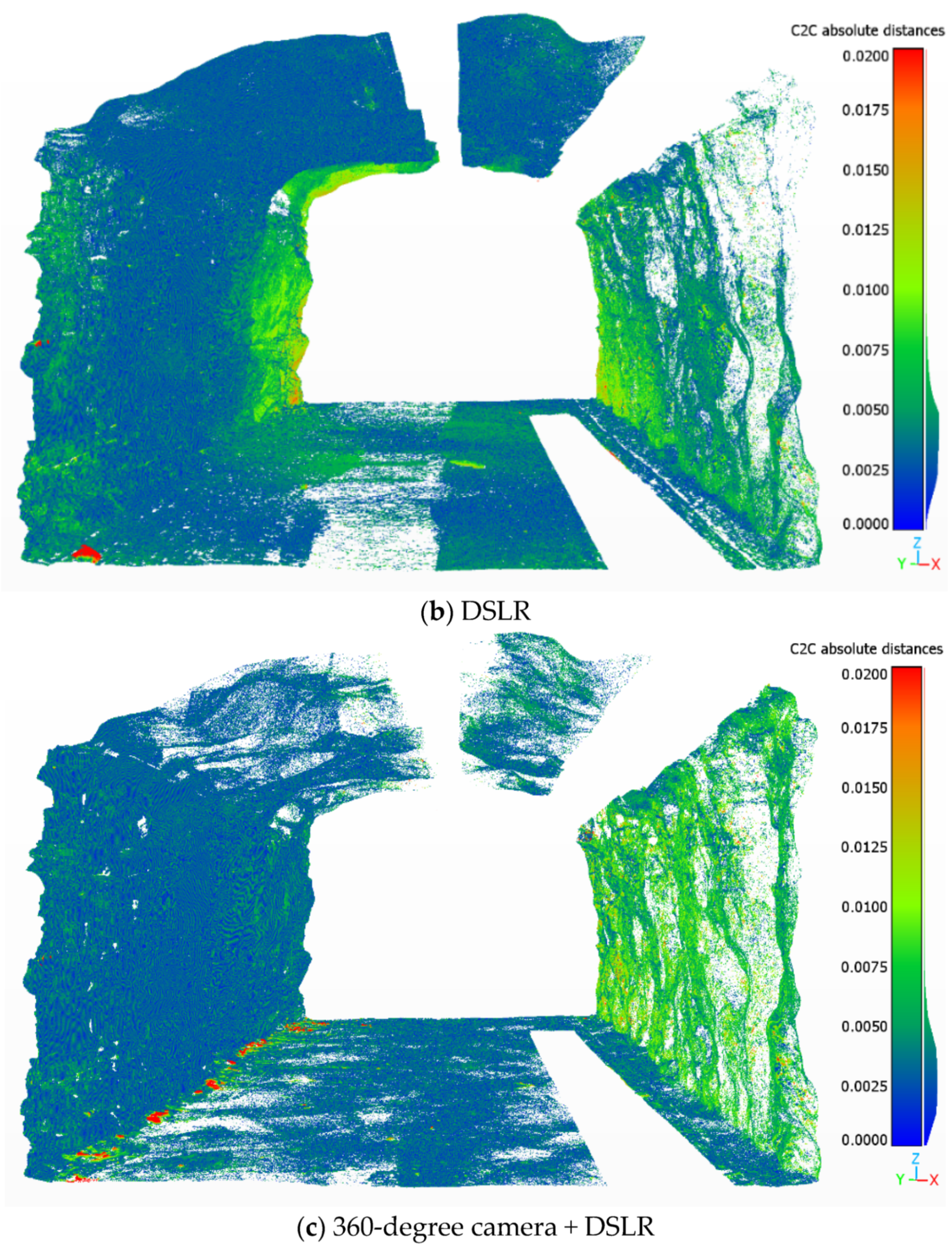
Figure 12.
Rock mass mapping window on the tunnel wall (a) with three extracted rock discontinuity sets (red, green, and blue colored points) extracted with the Discontinuity Set Extractor from the point clouds: (b) 360-degree model, (c) DSLR model, (d) 360-degree and HQ model, and (e) reference TLS model.

Figure 13.
Comparison of the orientation of discontinuity sets extracted from the 3D models using a semi-automatic method by [5], and conventional geological compass measurements.
Figure 13.
Comparison of the orientation of discontinuity sets extracted from the 3D models using a semi-automatic method by [5], and conventional geological compass measurements.

Table 1.
Image processing settings in Adobe Lightroom Classic.
| Setting Group | Parameter | Value |
|---|---|---|
| Basic delighting | Highlights | −100 |
| Shadows | 100 | |
| Sharpening | Amount | 60 |
| Radius | 0.5 | |
| Detail | 100 |
Table 2.
Alignment settings in RealityCapture photogrammetric software.
| Alignment Parameter | Value |
|---|---|
| Image overlap | Low |
| Max features per Mpx | 10,000 |
| Max features per image | 40,000 |
| Detector sensitivity | Medium |
| Preselector features | 10,000 |
| Image downscale factor | 1 |
| Maximal feature reprojection error [pixels] | 1.00 |
| Use camera positions | True |
| Lens distortion model | K + Brown4 with tangential2 |
Table 3.
Image acquisition time and surface point density results.
| Photogrammetric Method | 360 | DSLR | 360 + HQ |
|---|---|---|---|
| Number of images | 162 | 111 | 162 + 13 |
| Capture time | 10 min | 34 min | 10 + 4 min |
| Alignment time | 2 min 19 s | 1 min 17 s | 2 min 59 s |
| Mesh reconstruction and texturing time | 22 min 23 s | 49 min 04 s | 32 min 29 s |
| Overall processing time | 24 min 42 s | 50 min 21 s | 35 min 28 s |
| Surface point density | 20.7 pts/cm2 | 33.2 pts/cm2 | 87.4 pts/cm2 |
| Surface point density–mapping wall | 24.5 pts/cm2 | 24.2 pts/cm2 | 96.9 pts/cm2 |
Table 4.
Measured and calculated control distances and the RMSE.
| Measured Distance (m) | 360 | DSLR | 360 + HQ | TLS |
|---|---|---|---|---|
| 1.7594 | 1.7543 | 1.7561 | 1.7564 | 1.7574 |
| 5.3671 | 5.3690 | 5.3683 | 5.3703 | 5.3625 |
| 1.8094 | 1.8092 | 1.8072 | 1.8081 | 1.8025 |
| 1.7548 | 1.7623 | 1.7584 | 1.7596 | 1.7572 |
| 5.4670 | 5.4804 | 5.4643 | 5.4676 | 5.4545 |
| 1.4461 | 1.4500 | 1.4510 | 1.4515 | 1.4511 |
| 2.1470 | 2.1548 | 2.1579 | 2.1584 | 2.1542 |
| 5.3876 | 5.3816 | 5.3846 | 5.3861 | 5.3717 |
| 3.9992 | 4.0065 | 4.0074 | 4.0085 | 4.0157 |
| 4.4164 | 4.4340 | 4.4306 | 4.4322 | 4.4143 |
| 3.4650 | 3.4784 | 3.4716 | 3.4728 | 3.4637 |
| 4.4803 | 4.4914 | 4.4893 | 4.4908 | 4.4829 |
| 5.2344 | 5.2333 | 5.2361 | 5.2375 | 5.2215 |
| 5.2127 | 5.2169 | 5.2224 | 5.2237 | 5.2091 |
| 4.1423 | 4.1417 | 4.1479 | 4.1491 | 4.1431 |
| 2.4581 | 2.4639 | 2.4644 | 2.4652 | 2.4649 |
| 3.7464 | 3.7560 | 3.7576 | 3.7591 | 3.7548 |
| 5.6238 | 5.6257 | 5.6195 | 5.6205 | 5.6041 |
| 4.8475 | 4.8626 | 4.8561 | 4.8592 | 4.8421 |
| 2.4336 | 2.4353 | 2.4309 | 2.4322 | 2.4281 |
| 5.4793 | 5.4755 | 5.4757 | 5.4781 | 5.4773 |
| 9.6027 | 9.6078 | 9.6140 | 9.6176 | 9.6092 |
| 6.2157 | 6.2196 | 6.2217 | 6.2240 | 6.2155 |
| 7.9028 | 7.9295 | 7.9215 | 7.9243 | 7.9174 |
| 8.3790 | 8.3942 | 8.3925 | 8.3951 | 8.3924 |
| RMSE (m) | 0.0099 | 0.0082 | 0.0095 | 0.0090 |
Table 5.
Cloud-to-Cloud (C2C) distance measured between the point clouds and a reference laser scan.
Table 5.
Cloud-to-Cloud (C2C) distance measured between the point clouds and a reference laser scan.
| Photogrammetric Method | 360 | DSLR | 360 + HQ |
|---|---|---|---|
| Cloud-to-Cloud distance (RMS) (m) | 0.0046 | 0.0050 | 0.0043 |
| C2C (mean of a fitted Gauss distribution) (m) | 0.0040 ± 0.0048 | 0.0043 ± 0.0052 | 0.0038 ± 0.0042 |
Table 6.
Comparison of the mean orientation of discontinuity sets extracted from the 3D models using the semi-automatic method by [2], and manual compass measurements.
Table 6.
Comparison of the mean orientation of discontinuity sets extracted from the 3D models using the semi-automatic method by [2], and manual compass measurements.
| Joint Set | Dip Direction (°) | Abs. Diff. | Dip (°) | Abs. Diff. | |
|---|---|---|---|---|---|
| 360 | 1 | 327.5 | 2.3 | 85.8 | 3.2 |
| 2 | 55.9 | 3.0 | 83.4 | 4.5 | |
| 3 | 281.1 | 30.5 | 13.8 | 9.1 | |
| DSLR | 1 | 325.9 | 0.7 | 83.4 | 5.6 |
| 2 | 55.9 | 3.0 | 83.4 | 4.5 | |
| 3 | 293.4 | 18.2 | 20.5 | 15.8 | |
| 360 + HQ | 1 | 327.5 | 2.3 | 85.8 | 3.2 |
| 2 | 55.9 | 3.0 | 83.4 | 4.5 | |
| 3 | 281.0 | 30.6 | 7.5 | 2.8 | |
| TLS | 1 | 324.0 | 1.2 | 87.4 | 1.6 |
| 2 | 56.7 | 2.2 | 87.6 | 0.3 | |
| 3 | 287.7 | 23.9 | 8.6 | 3.9 | |
| Geological compass | 1 | 325.16 | 89.00 | ||
| 2 | 58.90 | 87.87 | |||
| 3 | 311.59 | 4.74 |
Publisher’s Note: MDPI stays neutral with regard to jurisdictional claims in published maps and institutional affiliations. |
© 2022 by the authors. Licensee MDPI, Basel, Switzerland. This article is an open access article distributed under the terms and conditions of the Creative Commons Attribution (CC BY) license (https://creativecommons.org/licenses/by/4.0/).
Share and Cite
MDPI and ACS Style
Janiszewski, M.; Torkan, M.; Uotinen, L.; Rinne, M. Rapid Photogrammetry with a 360-Degree Camera for Tunnel Mapping. Remote Sens. 2022, 14, 5494. https://doi.org/10.3390/rs14215494
AMA Style
Janiszewski M, Torkan M, Uotinen L, Rinne M. Rapid Photogrammetry with a 360-Degree Camera for Tunnel Mapping. Remote Sensing. 2022; 14(21):5494. https://doi.org/10.3390/rs14215494
Chicago/Turabian StyleJaniszewski, Mateusz, Masoud Torkan, Lauri Uotinen, and Mikael Rinne. 2022. "Rapid Photogrammetry with a 360-Degree Camera for Tunnel Mapping" Remote Sensing 14, no. 21: 5494. https://doi.org/10.3390/rs14215494
Note that from the first issue of 2016, this journal uses article numbers instead of page numbers. See further details here.