

A Multi-Path Encoder Network for GPR Data Inversion to Improve Defect Detection in Reinforced Concrete


1
State Key Laboratory of Coastal and Offshore Engineering, Dalian University of Technology, Dalian 116024, China
2
Research Institute of Dalian University of Technology in Shenzhen, Shenzhen 518057, China
3
School of Civil Engineering, Dalian University, Dalian 116622, China
*
Author to whom correspondence should be addressed.
Remote Sens. 2022, 14(22), 5871; https://doi.org/10.3390/rs14225871
Submission received: 28 September 2022
/
Revised: 15 November 2022
/
Accepted: 17 November 2022
/
Published: 19 November 2022
(This article belongs to the Special Issue Radar Techniques for Structures Characterization and Monitoring)
Abstract
:Ground penetrating radar (GPR) has been extensively used in the routine inspection of reinforced concrete structures. However, the signatures in GPR images are reflected electromagnetic waves rather than their actual shapes. The interpretation of GPR data is a mandatory but time- and labor-consuming task. Furthermore, the rebars in the near-surface of concrete cause clutter in the GPR images, which hinders the interpretation of GPR data. This work presents a deep learning network to invert GPR B-scan images to permittivity maps of subsurface structures. The proposed network has a multi-path encoder which enables the network to leverage three kinds of GPR data: the original, migrated, and encoder–decoder-processed GPR data. Each type of processing method is designed to serve a different purpose: the original GPR images retain all the waveforms; the migration method intensifies the vertices of the subsurface anomalies; the encoder–decoder network suppresses rebar clutter and enhances the visibility of the defect echoes. The outputs of three processing methods are jointly used to interpret GPR B-scan images. We demonstrated the superiority of the proposed network by comparing it with a network with a single-path encoder. We also validated the proposed network with synthetic and experimental GPR data. The results indicate that the proposed network effectively reconstructs the defects in the reinforced concrete.
1. Introduction
Most of the concrete structures in service have various kinds of defects, such as voids, cracks, delamination, and untightness, which are caused by environmental factors, inadequate construction, or poor maintenance. To prevent these defects from jeopardizing the security of concrete structures, it is necessary to conduct routine inspections and assessments. Ground penetrating radar (GPR), a non-destructive testing method, has been extensively used in concrete-structure inspection because of its desirable reliability and effectiveness [1,2,3,4,5,6]. As a near-surface-level geophysical detection technique, GPR deduces the subsurface’s condition by transmitting high-frequency electromagnetic waves into the structure and receiving echoes in which there are electromagnetic property contrasts. Several received echoes form a GPR B-scan image (radargram), and hereafter the technicians deduce the structure of the subsurface medium according to the characteristics of the reflected waveforms. However, the interpretation of GPR data is a challenging task. The obtained GPR data are reflected electromagnetic waveforms of the subsurface, which are difficult to interpret. This makes the experience and expertise of technicians essential to identify targets from GPR images correctly [7]. Furthermore, when the amount of data is enormous, the interpretation of GPR data becomes a time- and labor-consuming task. Automatic identification methods for GPR data are urgently needed to improve the efficiency and accuracy.
With the emergence of convolutional neural networks (CNNs) [8,9], the deep learning (DL) methods have achieved state-of-art performance in signal and image processing and have been applied to GPR data interpretation [10]. Liu et al. [11] proposed an automatic detection and localization method using DL and migration. This method can locate rebars in real time with acceptable accuracy. In order to predict the sizes, shapes, and locations of the subsurface defects, Yang et al. [12] used a segmentation network named Segnet to map the tunnel-lining internal defects. Segnet can segment the defects in a tunnel lining with better performance than U-net and DeepLab V3+. Qin et al. [13] introduced a Mask-RCNN based framework to identify steel ribs, voids, and the thicknesses of tunnel linings. This method recognized designated targets with high accuracy yet was not developed for interpreting the actural shapes. Liu et al. [14] proposed a deep neural network referred to as GPRInvNet to tackle the challenges of mapping the GPR B-scan data to complex permittivity maps of subsurface structures. GPRInvNet can establish a spatial alignment between time-series B-scan data and spatial permittivity maps. Validation was conducted on both the finite-difference time-domain (FDTD) synthetic and physical model testing. The results show that the network is able to reconstruct high-quality relative permittivity maps of subsurface structure from GPR B-scan data. To make the DL network have the ability to invert GPR data with long survey lines, Wang et al. [15] proposed GPRI2Net. GPRI2Net combines a DenseUnet and a recurrent neural network to exploit the contextual information contained between each data segment in a consecutive and long survey line.
Although the DL methods have demonstrated extraordinary abilities in GPR data interpretation, there are still challenges that hinder the further applications of deep learning methods. Since there are rebars in the near-surface of a concrete structure, the identification of subsurface defects is more difficult. The rebars in the concrete structure act as scatters that generate clutter in GPR profiles and mask the target signatures, making defect echoes beneath the rebars hard to distinguish. In addition, there are many different data processing schemes for GPR B-scan data, and each serves a different purpose. However, most of the existing DL methods only use the original GPR data with gain and noise reduction operations. The GPR data processing step is instrumental for interpreting GPR data. However, current methods cannot effectively utilize the various information contained in GPR data with different data processing methods.
To cope with these problems, many researchers have tried to use different signal processing methods to suppress rebar clutters and decode radargrams. Xiao et al. [16] proposed a multi-bandpass filter technique to suppress clutters in GPR profiles caused by periodic elements in the near-surface. Wu et al. [17] reduced rebar echoes in GPR data using hyper-curvelet transform. Wang et al. [18] proposed a supervised deep learning network for rebar-clutter removal and defect-echo enhancement in GPR images. The results show that the DL-based method is promising for rebar-clutter removal according to its performance and processing speed. However, any supervised learning network has a high level of dependence on a paired dataset. Wang et al. [19] proposed an unsupervised DL network called the RCE-GAN to remove rebar clutters. Compared to the network proposed by Wang et al. [18], the RCE-GAN does not need a paired dataset to train the network. Hence, the RCE-GAN is easier to implement because of its lower demand on the training dataset. The detection accuracy of the YOLOv4 network on the RCE-GAN-processed data was improved by 11.9% compared to that on the unprocessed data. Dinh et al. [20,21] combined migration and DL to locate rebars in bridge decks. The migration method concentrates the rebar reflected energy to the vertices, which is beneficial to locating rebars in the concrete [20]. To sum up, the GPR data processing step is instrumental and can improve detection accuracy significantly.
To jointly utilize the strengths of both conventional signal processing and deep learning methods, we proposed a deep learning network to invert processed GPR data to their dielectric properties. The proposed network has three encoder paths and uses the information of three types of GPR data simultaneously. In this work, we first introduce the design of inversion network. Then, we present the three kinds of GPR data and their functions in GPR data inversion. Next, we describe the training and validation of the performance of the network using synthetic GPR data. A comparison study is also reported between the proposed network and a network with a single-path encoder. Finally, we describe a physical experiment that validates the applicability of the proposed network.
2. Methodology
The proposed network G utilizes the original GPR data O, the migrated GPR data M, and the encoder–decoder-processed GPR data E to infer the permittivity map P of the concrete structure, which can be denoted by the following expression:
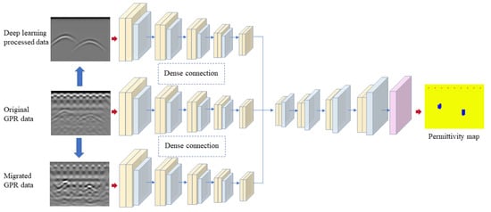
The network’s structure is illustrated in Figure 1. Three categories of GPR data, including the original, migrated, and encoder–decoder-processed GPR data, are used as the input for the network. A three-path encoder is implemented to process the three kinds of GPR images simultaneously, which extracts three times more information than processing a single GPR image. Dense connections are set between the adjacent encoder paths and allow the network to take advantage of the spatially related information. Then, a decoder network is used to merge all the features obtained by the multi-path encoder and output a permittivity map in accordance with the GPR image.
2.1. Multi-Path Encoder
On the whole, the inversion network has an encoder–decoder structure with three encoder paths. Each encoder path is designed to process one kind of input data. In each encoder path, the input data are first resized to and then passed through a series of convolutional blocks and down-sampling layers. Each convolutional block consists of two convolutional layers, a batch-norm layer, a drop-out layer, and a rectified linear unit (ReLU) layer. All convolution operations apply spatial filters with 1 stride, a dropout rate, and the down-sampling factor of 2. In total, there are four convolutional blocks and four max-pooling layers in each encoder path.
The original, migrated, and encoder–decoder-processed GPR data are used as the inputs of the three encoder paths, respectively. Note that as the migrated and encoder–decoder-processed data are obtained from the original GPR data, the three kinds of GPR data are spatially related, although they are processed with different methods and have different roles. Therefore, we use dense connections between adjacent encoder paths to establish a lateral relationship among the three encoder paths [22], as shown in Figure 1b.
Let denote the output of the layer in the first encoder path, be the mapping function, and and signify the output and mapping function of the adjacent encoder path. Thus, the output of the layer can be expressed as
In this kind of connection, all feature outputs are concatenated in a feed-forward manner. Each convolutional block receives the results obtained from the previous one and its adjacent encoder paths. With the dense connections, the network can learn complex relationships between three different kinds of GPR data.
After a series of processing and feature-fusion steps, the encoder produces deep features. Then, a decoder is used to amplify the compressed features to a permittivity map with the same size as the original GPR images by the deconvolutional blocks and up-sampling layers. A total of four deconvolutional blocks with kernels of three and four up-sampling blocks are employed in the decoder network. There is a great deal of low-level information shared between the encoder and decoder, such as the locations of the objects [23]. Therefore, we shuttle the outputs of the convolutional blocks in each layer of the encoder directly across the net to the corresponding layer of the decoder. After processing by the last layer of the decoder, we apply a convolutional layer to map the features to the number of output channels, followed by a anh function.
2.2. Adversarial Learning and Loss Function
In the training process, we calculate the difference between the outputs of the encoder–decoder network and the ground truth to optimize the network. The L1-distance loss is expressed as
where x represents the input GPR data, y represents the ground truth data, G denotes the encoder–decoder network, and G(x) represents the network’s output. The L1-distance loss makes the data reconstructed by the network close to the ground truth in an L1 sense. However, in the process of training, we found that if we only applied L1-distance loss, the network generated blurry results with a roughly correct distribution of relative permittivity values, but the high-frequency details were missing. Thus, we introduced a discriminator to the network. The encoder–decoder network (generator) and the discriminator together form a generative adversarial network (GAN). Now the generator and discriminator are trained jointly, and loss function of the GAN is signified as follows:
In this loss function, the generator aims at minimizing this loss against an adversarial discriminator that tries to maximize it: the generator G is trained to produce the permittivity map that is indistinguishable from the real distribution, and the discriminator D is trained synchronously to discern the generator’s fake. As the generator has already generated blurry results, it is wise to make the discriminator only model high-frequency features. Like the method used in [24], instead of taking the entire image as input, we make the GAN discriminator only classify if the patches in an image are real or fake. This motivates the GAN discriminator to only model high-frequency features. We run this discriminator convolutionally across the image, averaging all responses to provide the ultimate output of D. The structure of the GAN discriminator is shown in Figure 2. The combination of the L1-distance loss and GAN loss is used as the loss function of our inversion network:
where the is a balancing parameter that controls the relative importance of the two parts. In our study, to correctly reconstruct the permittivity map has higher priority, so the L1-distance loss should account for a larger share of the loss function. The is taken as 10 in this study.
3. Data Preparation and Processing
The proposed network has a multi-path encoder, which enables it to leverage three kinds of GPR data: the original GPR data, the migrated GPR data, and the encoder–decoder-processed GPR data. Each GPR data serves a different purpose: the original GPR images retain all the waveforms; the migration method intensifies the vertices of the subsurface anomalies; the encoder–decoder is a deep learning network used to suppress rebar clutter and enhance the visibility of the defect echoes. To train the network, we need to prepare sufficient GPR data. The prepared GPR data are shown in Figure 3.
3.1. Original GPR Data
We created numerical models to generate synthetic GPR data to train the proposed network. As shown in the first column of Figure 3, the dimensions of the models are 1.0 m × 2.0 m (height × width). There are three kinds of concrete defects with irregular geometries in the synthetic model, which are voids, cracks, and untightness. In the near-surface of the concrete is a row of rebars. We performed simulations using the gprMax program, a Python-based FDTD solver of Maxwell’s equations to create synthetic GPR data [25]. The center frequency of the source wavelet is 500 MHz, the time window is set to 20 ns, and the trace interval is 0.01 m. We define the concrete with , S/m, and air-filled defects with , S/m. By FDTD simulations, we obtained a total of 700 GPR images and their corresponding permittivity maps, 600 of which were used to train the network and the rest for validation. The training dataset contains three types of defects, including voids, cracks, and untightness. The geometries of the defects are distributed randomly in the numerical models. For each type of defect, 200 synthetic GPR images were collected. Then, we applied basic data-processing operations using time-zero correction and time-varying gain on all the GPR data. The processed GPR data are shown in the second column of Figure 3, which were used as the original GPR data for the inversion.
3.2. Migrated GPR Data
In a typical GPR B-scan image, any anomalies within the region of detection present as hyperbolas. Detailed information of the subsurface anomalies, such as their depth, size, and reflected amplitude are hard to represent in the GPR image due to the long tails of the hyperbola. It is a common practice to use the migration method in GPR data processing. Its purpose is to migrate the unfocused space-time GPR image to a focused one that demonstrates the object’s actual location and size together with its amplitude [26].
In this research, we used Stolt migration [27] to intensify the hyperbolas in the GPR B-scan images. Stolt migration is a wave-equation-migration-based algorithm that uses the wave equation to back-propagate the recorded wave. Stolt migration takes the advantage of Kirchhoff’s migration and runs faster by employing the fast Fourier transform. When performing the Stolt migration process, it is important to select a proper migration velocity. If the selected velocity is lower or higher than the true velocity, it may cause “under-migrated” or “over-migrated” GPR data. Figure 4 demonstrates the effect of migration with different velocities. Figure 4a,b depict the permittivity map and the synthetic GPR image before migration, and Figure 4c–e are the migrated GPR images using the correct velocity value (0.096 m/ns), a lower velocity value (0.080 m/ns), and a higher velocity value (0.140 m/ns), respectively. Figure 4d,e are typical “under-migrated” and “over-migrated” GPR images. When the migration velocity is inappropriate, the focus effect of the migration method is reduced greatly. In this work, we determined the migration velocity using the minimum entropy technique [28,29]. Suppose a migrated GPR B-scan image is expressed as a two-dimensional matrix X.
where indicates the i-th sampling points of the j-th trace and is the j-th trace. The entropy of migrated data is calculated as
According to the definition, the maximum value of entropy for each trace is one when the data contain only a pulse peak with a single-unit amplitude. In terms of the migrated data, the lower its entropy is, the better the focus effect of the migration method. We tune the migration velocity and calculate the entropy until a point where the the entropy reaches its minimum. In this research, the minimum entropy was 0.539, obtained at a migration velocity of 0.096. As shown in Figure 4c, after migration with the correct velocity, the true locations of anomalies ended up with intensity values. The information of the anomalies, including their depth, size, and reflected amplitude, can be better determined in the migrated GPR profile.
3.3. Deep-Learning-Processed GPR Data
Due to the fact that there are rebars in the near-surface of the reinforced concrete, the reflections of the subsurface objects become difficult to discern because rebar clutters in GPR images mask the reflected waves of the inner structural defects. In our previous study [19], deep learning methods have shown their effectiveness for rebar clutter removal and defect echo enhancement in GPR B-scan images. Thus, in this work, we used the network proposed in [19] to process GPR data.
The configuration of the rebar clutter removal network is shown in Figure 5, which is a supervised learning network with an encoder–decoder structure with skip connections. The input GPR images are first resized to 512 × 512, then passed through a series of convolutional and down-sampling layers until a bottleneck layer, at which point the process is then reversed. There are four convolutional blocks and four max-pooling layers in the encoder, and four deconvolutional blocks and four up-sampling blocks in the decoder. All convolutions are 3 × 3 spatial filters with one stride. The down-sampling and up-sampling factors are two in the encoder and decoder, respectively. After the last layer of the decoder, a convolution operation is applied to map the features to the number of output channels, followed by atTanh function. The output of the network is a GPR image without rebar clutters and is shown in the fourth column of Figure 3.
In the training process, the GPR data obtained by the FDTD simulations with forward model constructed without rebars were taken as the ground-truth images. The network’s output was compared with the ground truth to compute the loss value to optimize the network. We combined the L1-distance and structural similarity (SSIM) loss to form the loss function of the network, as shown in the following equations.
where x is the output of the network, y is the ground truth, and and represent the mean values of x and y, respectively. and denote the standard deviation of x and y, and signifies the covariance of x and y.
4. Synthetic Example
In this section, we use synthetic examples to demonstrate the applicability of the inversion network. As illustrated in the previous section, we used the 600 GPR images produced by FDTD simulations to train the network and the rest of 100 GPR images for testing. In the synthetic examples, three types of defects—voids, cracks, and untightness—are considered as potential targets to be identified.
4.1. Network Training
The training process was implemented on the Pytorch framework using an Intel Xeon (R) Gold 6266C CPU workstation with 192 GB RAM and a RTX 3080 GPU. We used the Adam solver as the optimizer [30], with the learning rate and decay rate of first-order momentum being 0.0002 and 0.5, respectively. The batch size was set to 8. We trained the network for 200 epochs, and the training process lasted for 3.5 h. The loss curve during the training process is shown in Figure 6.
4.2. Results
The inversion results on the testing dataset are shown in Figure 7. The first three columns present the original, migrated, and deep-learning-processed GPR images of void, crack, and untightness defects. The fourth column shows the ground-truth permittivity maps of the three defects. The fifth column displays the inversion results of the proposed network, which reconstructed the defects correctly. For comparison, we trained a single encoder network that utilizes only the original GPR images to invert the permittivity maps. The results are illustrated in the last column of Figure 7.
We also used the SSIM and intersection over union (IoU) as the indicators to quantitatively evaluate the inversion performance of the network. The SSIM was used to evaluate the similarity between the inverted permittivity map and the ground-truth image, whereas the IoU was used to measure the ratio of the area of intersection to the area of union. The comparison of the SSIM and IoU of the proposed method and the single encoder network is demonstrated in Figure 8.
In Figure 7, we can see that both networks inverted the rebar positions accurately. This is because the vertices of the rebars in the near-surface are clear. The average IoU values of both networks are one (see Figure 8b). Both networks are competent for rebar detection and localization. As for the inversion of defects, the results are different. It can be seen in Figure 7a that both the proposed network and compared network can complete the inversion task, but the accuracies of the inverted results have subtle differences. The average IoU values of the proposed network and the compared network for the void defects were 0.6108 and 0.5088, respectively. As shown in Figure 7b, the proposed network detects the presence of the crack yet does not invert the crack completely. This is because the reflection amplitude of defects is weak and easy to be masked by the rebar clutter, even though we enhanced the features of cracks in the GPR images through migration and deep learning methods. The inversion result is worse for the compared network, and no defects were found at all. The average IoU values of the two networks for cracks were 0.4288 and 0, respectively. In Figure 7c, we can see that both the proposed and the compared network detect the untightness correctly. However, it is quite evident that the defect area inverted by the proposed network is closer to the ground truth. The network with a single encoder is affected by rebar clutters in the GPR data and led to undesired results in the inversion task. The average IoUs of two networks for the untightness were 0.8397 and 0.3699, respectively.
Figure 8a compares the SSIM values of the proposed network and the compared network for the different anomalies. As concrete accounts for most of the model’s area, both the networks can achieve high SSIM values. The proposed network inverses the defects better, and hence achieves higher scores. For the IoU values presented in Figure 8b, the proposed network outperformed the compared network by a large margin in all the defect cases. We can therefore conclude that the proposed network performs better than the single-path encoder on the synthetic dataset.
5. Laboratory Experiment
In this section, we demonstrate the effectiveness of our inversion approach using the GPR data acquired from a physical model experiment to validate the practicality of the proposed method on real-world GPR data.
As shown in Figure 9a, we built a reinforced concrete model with dimensions of 1.0 m × 2.0 m (height × width). From the top to bottom, the model consisted of three layers, including reinforced concrete, plain concrete, and sand with thicknesses of 0.6, 0.25, and 0.15 m, respectively. Inside of the reinforced concrete layer, there were three voids denoted as V1, V2, and V3. The voids were made of cubic wooden boxes, and the side lengths were 0.2, 0.1, and 0.2 m, respectively. The burial depths of three voids were 0.37, 0.47, and 0.36 m, respectively. Inside this layer there were two rows of equally spaced rebars, 22 mm in diameter, and with a spacing of 33 cm. The depths of the two layers of rebars were 5 and 55 cm, respectively. We used the pulse EKKO PRO GPR system equipped with a 500 MHz center frequency antenna to obtain GPR data. The time window was set as 30 ns, the sampling rate was 100 trace/m, and the length of the survey line was 2.0 m.
As shown in Figure 9b, we obtained a raw GPR image from the model experiment. Prior to inverting the GPR image using the proposed network, pre-processing was performed on the raw data. The pre-processing operations included time-zero correction, direct-current (DC) shift removal, time-varying gain, frequency filtering, and time window trimming. First, we adjusted the starting time of the GPR data to view the air–concrete surface. Then, we removed the DC component by subtracting the mean value of each trace. Next, we used the time-varying gain with the exponential function to compensate for the attenuation of GPR signals. After that, we suppressed the noise using a 1D band-pass filter with lower and upper cut-off frequencies of 200 and 650 MHz, respectively. Finally, we trimmed the time window to 20 ns.
After pre-processing, we obtained the original GPR data for the inversion plotted in Figure 10a. Next, we migrated the original GPR data with migration velocity of 0.094 m/ns and achieved the minimum entropy value of 1.2866. The migrated GPR image is demonstrated in Figure 10b. We also processed the original GPR data using the rebar elimination network and obtained the rebar clutter eliminated GPR image depicted in Figure 10c.
We fed the three GPR images into the proposed network and obtained the inversion results shown in Figure 10d. The relative positions of all three voids are almost identical to those in the ground truth. Additionally, all eight rebars were reconstructed in the correct locations. The sizes of the voids V1, V2, and V3 in the inverted permittivity map were , , and cm (width × height), respectively. Compared with the inverted positions, the accuracy of the void sizes is lower, which is caused mainly by two reasons: (1) Limited by time, cost, and other factors, we only used the FDTD synthetic GPR data as the training data. The FDTD model we built is different from the real situation, due to the inhomogeneity of the concrete medium, the attenuation of the signal, electromagnetic interference, etc. (2) The quality of the deep-learning-processed GPR data is affected by rebar clutters in the original data. However, the result is still promising, since all the voids were successfully reconstructed in their correct positions. More high-quality and well-labeled training data are needed to improve the performance of the proposed network on real-world GPR data.
6. Conclusions
In this research, a novel deep learning network with a multi-path encoder was proposed for the interpretation of GPR data. The network takes three kinds of GPR data as the input and outputs the permittivity maps of the subsurface. With the multi-path encoder, the network makes use of the information contained in the three types of GPR data all at once. The dense connection between the adjacent encoder paths makes the network take advantage of the spatially related information. Compared to conventional neural networks that only utilize one type of data, the proposed network has improved the inversion accuracy. On the synthetic GPR dataset, the average IoUs of the proposed network were 0.6108, 0.4288, and 0.8397 for void, crack, and untightness detection, higher than those of the conventional single-path encoder network, which were 0.5088, 0, and 0.3699, respectively. We also verified the proposed network on real-world data obtained from a physical experiment, in which the network detected the near-surface rebars and voids precisely.
Limited by time and cost, we collected an insufficient amount of real-world GPR data. Future directions of this research include: (1) to design a physical model to obtain sufficient high-quality and well-labeled GPR data to train and validate the proposed network; and (2) to improve the FDTD simulation method to create synthetic GPR data with high fidelity.
Author Contributions
Conceptualization, methodology, writing—original draft preparation, Y.W.; software, data curation, validation, H.Q.; writing—review and editing, F.M. All authors have read and agreed to the published version of the manuscript.
Funding
This research was funded by the National Natural Science Foundation of China (grant number 41904095) and Special Funds for Central Government Guidance to Local Governments for Science and Technology Development in Shenzhen (2021Szvup020).
Data Availability Statement
GPR profile data in this artical can be publicly accessed through https://github.com/yxwang1794/the-data-of-multi-path-encoder-network-for-gpr-inversion (accessed on 27 September 2022).
Conflicts of Interest
The authors declare no conflict of interest.
References
- Alani, A.M.; Tosti, F. GPR applications in structural detailing of a major tunnel using different frequency antenna systems. Constr. Build. Mater. 2018, 158, 1111–1122. [Google Scholar] [CrossRef]
- Wai-Lok Lai, W.; Dérobert, X.; Annan, P. A review of ground penetrating radar application in civil engineering: A 30-year journey from locating and testing to imaging and diagnosis. NDT E Int. 2018, 96, 58–78. [Google Scholar] [CrossRef]
- Lalagüe, A.; Lebens, M.A.; Hoff, I.; Grøv, E. Detection of rockfall on a tunnel concrete lining with Ground-Penetrating Radar (GPR). Rock Mech. Rock Eng. 2016, 49, 2811–2823. [Google Scholar] [CrossRef]
- Munda, S.; Zanzi, L.; Arosio, D. GPR investigations to assess the state of damage of a concrete water tunnel. J. Environ. Eng. Geophys. 2012, 17, 159–169. [Google Scholar] [CrossRef] [Green Version]
- Qin, H.; Xie, X.; Tang, Y.; Wang, Z. Experimental study on GPR detection of voids inside and behind tunnel linings. J. Environ. Eng. Geophys. 2020, 25, 65–74. [Google Scholar] [CrossRef]
- Qin, H.; Tang, Y.; Wang, Z.; Xie, X.; Zhang, D. Shield tunnel grouting layer estimation using sliding window probabilistic inversion of GPR data. Tunn. Undergr. Space Technol. 2021, 112, 103913. [Google Scholar] [CrossRef]
- Ozkaya, U.; Melgani, F.; Belete Bejiga, M.; Seyfi, L.; Donelli, M. GPR B scan image analysis with deep learning methods. Measurement 2020, 165, 107770. [Google Scholar] [CrossRef]
- LeCun, Y.; Bengio, Y.; Hinton, G. Deep learning. Nature 2015, 521, 436–444. [Google Scholar] [CrossRef]
- Krizhevsky, A.; Sutskever, I.; Hinton, G.E. ImageNet classification with deep convolutional neural networks. Adv. Neural Inf. Process. Syst. 2012, 25, 1097–1105. [Google Scholar] [CrossRef] [Green Version]
- Tong, Z.; Gao, J.; Yuan, D. Advances of deep learning applications in ground-penetrating radar: A survey. Constr. Build. Mater. 2020, 258, 120371. [Google Scholar] [CrossRef]
- Liu, H.; Lin, C.; Cui, J.; Fan, L.; Xie, X.; Spencer, B.F. Detection and localization of rebar in concrete by deep learning using ground penetrating radar. Autom. Constr. 2020, 118, 103279. [Google Scholar] [CrossRef]
- Yang, S.; Wang, Z.; Wang, J.; Cohn, A.G.; Zhang, J.; Jiang, P.; Nie, L.; Sui, Q. Defect segmentation: Mapping tunnel lining internal defects with ground penetrating radar data using a convolutional neural network. Constr. Build. Mater. 2022, 319, 125658. [Google Scholar] [CrossRef]
- Qin, H.; Zhang, D.; Tang, Y.; Wang, Y. Automatic recognition of tunnel lining elements from GPR images using deep convolutional networks with data augmentation. Autom. Constr. 2021, 130, 103830. [Google Scholar] [CrossRef]
- Liu, B.; Ren, Y.; Liu, H.; Xu, H.; Wang, Z.; Cohn, A.G.; Jiang, P. GPRInvNet: Deep learning-based ground-penetrating radar data inversion for tunnel linings. IEEE Trans. Geosci. Remote Sens. 2021, 59, 8305–8325. [Google Scholar] [CrossRef]
- Wang, J.; Liu, H.; Jiang, P.; Wang, Z.; Sui, Q.; Zhang, F. GPRI2Net: A deep-neural-network-based ground penetrating radar data inversion and object identification framework for consecutive and long survey lines. IEEE Trans. Geosci. Remote Sens. 2022, 60, 5106320. [Google Scholar] [CrossRef]
- Xiao, J.; Liu, L. Suppression of clutters caused by periodic scatterers in GPR profiles with multibandpass filtering for NDT&E imaging enhancement. IEEE J. Sel. Top. Appl. Earth Obs. Remote Sens. 2017, 10, 4273–4279. [Google Scholar] [CrossRef]
- Wu, R.; Zhong, Y.; Liu, J. Rebar echo detection and suppression in runway using GPR. In Proceedings of the 2011 IEEE CIE International Conference on Radar, Chengdu, China, 24–27 October 2011; Volume 2, pp. 1339–1342. [Google Scholar] [CrossRef]
- Wang, J.; Chen, K.; Liu, H.; Zhang, J.; Kang, W.; Li, S.; Jiang, P.; Sui, Q.; Wang, Z. Deep learning-based rebar clutters removal and defect echoes enhancement in GPR images. IEEE Access 2021, 9, 87207–87218. [Google Scholar] [CrossRef]
- Wang, Y.; Qin, H.; Tang, Y.; Zhang, D.; Yang, D.; Qu, C.; Geng, T. RCE-GAN: A rebar clutter elimination network to improve tunnel lining void detection from GPR images. Remote Sens. 2022, 14, 251. [Google Scholar] [CrossRef]
- Dinh, K.; Gucunski, N.; Duong, T.H. Migration-based automated rebar picking for condition assessment of concrete bridge decks with ground penetrating radar. NDT E Int. 2018, 98, 45–54. [Google Scholar] [CrossRef]
- Dinh, K.; Gucunski, N.; Duong, T.H. An algorithm for automatic localization and detection of rebars from GPR data of concrete bridge decks. Autom. Constr. 2018, 89, 292–298. [Google Scholar] [CrossRef]
- Dolz, J.; Gopinath, K.; Yuan, J.; Lombaert, H.; Desrosiers, C.; Ayed, I.B. HyperDense-Net: A hyper-densely connected CNN for multi-modal image segmentation. IEEE Trans. Med. Imaging 2019, 38, 1116–1126. [Google Scholar] [CrossRef] [PubMed] [Green Version]
- Ronneberger, O.; Fischer, P.; Brox, T. U-Net: Convolutional Networks for Biomedical Image Segmentation. In Proceedings of the Medical Image Computing and Computer-Assisted Intervention, Munich, Germany, 5–9 October 2015; pp. 234–241. [Google Scholar] [CrossRef] [Green Version]
- Isola, P.; Zhu, J.; Zhou, T.; Efros, A.A. Image-to-image translation with conditional adversarial networks. In Proceedings of the 2017 IEEE Conference on Computer Vision and Pattern Recognition (CVPR), Honolulu, HI, USA, 21–26 July 2017; pp. 5967–5976. [Google Scholar] [CrossRef] [Green Version]
- Warren, C.; Giannopoulos, A.; Giannakis, I. gprMax: Open source software to simulate electromagnetic wave propagation for Ground Penetrating Radar. Comput. Phys. Commun. 2016, 209, 163–170. [Google Scholar] [CrossRef] [Green Version]
- Özdemir, C.; Demirci, S.; Yiǧit, E.; Yilmaz, B. A review on migration methods in B-Scan ground penetrating radar imaging. Math. Probl. Eng. 2014, 2014, 280738. [Google Scholar] [CrossRef] [Green Version]
- Stolt, R.H. Migration by fourier transform. Geophysics 1978, 43, 23–48. [Google Scholar] [CrossRef]
- Zhou, H.; Wan, X.; Li, W.; Jiang, Y. Combining F-K filter with minimum entropy Stolt migration algorithm for subsurface object imaging and background permittivity estimation. Procedia Eng. 2011, 23, 636–641. [Google Scholar] [CrossRef] [Green Version]
- Xu, X.; Miller, E.; Rappaport, C. Minimum entropy regularization in frequency-wavenumber migration to localize subsurface objects. IEEE Trans. Geosci. Remote Sens. 2003, 41, 1804–1812. [Google Scholar] [CrossRef]
- Kingma, D.P.; Ba, J. Adam: A Method for Stochastic Optimization. arXiv 2017, arXiv:1412.6980. [Google Scholar]
Figure 1.
Network configuration. (a) Overall structure of the network; (b) detailed information of the dense connections between the adjacent encoder paths.
Figure 1.
Network configuration. (a) Overall structure of the network; (b) detailed information of the dense connections between the adjacent encoder paths.

Figure 2.
Structure of the GAN discriminator.

Figure 3.
Dataset preparation: (a) synthetic model with void defects; (b) synthetic model with cracks; (c) synthetic model with untight concrete. The images of the first column are the permittivity maps of the synthetic models; the second column depicts the original B-scan images produced by FDTD simulations; the third and forth columns signify the migrated and deep-learning-processed GPR images.

Figure 4.
Stolt migration with different velocities: (a) permittivity map, (b) original B-scan GPR image, (c) migration with the correct velocity value (0.096 m/ns), (d) migration with a lower velocity value (0.080 m/ns), and (e) migration with a higher velocity value (0.140 m/ns).
Figure 4.
Stolt migration with different velocities: (a) permittivity map, (b) original B-scan GPR image, (c) migration with the correct velocity value (0.096 m/ns), (d) migration with a lower velocity value (0.080 m/ns), and (e) migration with a higher velocity value (0.140 m/ns).

Figure 5.
Architecture of the deep learning network for rebar clutter removal.

Figure 6.
The loss curve of the network training process.

Figure 7.
Inversion results on the synthetic dataset: (a) synthetic data with void defects; (b) synthetic data with cracks; (c) synthetic data with untightness. The first three columns depict the original B-scan, migrated, and deep-learning-processed GPR images, respectively, as the input data. The fourth column shows the ground truth permittivity maps. The last two columns depict the inversion results of the proposed method and the single encoder network.

Figure 8.
The SSIM and IoU of the proposed network and compared network: (a) SSIM value, (b) IoU value.
Figure 8.
The SSIM and IoU of the proposed network and compared network: (a) SSIM value, (b) IoU value.

Figure 9.
Laboratory model for real-world GPR data acquisition: (a) cross-section of the model and (b) collected raw GPR data.
Figure 9.
Laboratory model for real-world GPR data acquisition: (a) cross-section of the model and (b) collected raw GPR data.

Figure 10.
Inversion results of the laboratory experiment: (a) original B-scan GPR image, (b) migrated GPR image, (c) the deep-learning-processed GPR image, and (d) the inverted permittivity map using the proposed network.
Figure 10.
Inversion results of the laboratory experiment: (a) original B-scan GPR image, (b) migrated GPR image, (c) the deep-learning-processed GPR image, and (d) the inverted permittivity map using the proposed network.

Publisher’s Note: MDPI stays neutral with regard to jurisdictional claims in published maps and institutional affiliations. |
© 2022 by the authors. Licensee MDPI, Basel, Switzerland. This article is an open access article distributed under the terms and conditions of the Creative Commons Attribution (CC BY) license (https://creativecommons.org/licenses/by/4.0/).
Share and Cite
MDPI and ACS Style
Wang, Y.; Qin, H.; Miao, F. A Multi-Path Encoder Network for GPR Data Inversion to Improve Defect Detection in Reinforced Concrete. Remote Sens. 2022, 14, 5871. https://doi.org/10.3390/rs14225871
AMA Style
Wang Y, Qin H, Miao F. A Multi-Path Encoder Network for GPR Data Inversion to Improve Defect Detection in Reinforced Concrete. Remote Sensing. 2022; 14(22):5871. https://doi.org/10.3390/rs14225871
Chicago/Turabian StyleWang, Yuanzheng, Hui Qin, and Feng Miao. 2022. "A Multi-Path Encoder Network for GPR Data Inversion to Improve Defect Detection in Reinforced Concrete" Remote Sensing 14, no. 22: 5871. https://doi.org/10.3390/rs14225871
Note that from the first issue of 2016, this journal uses article numbers instead of page numbers. See further details here.