Evaluation of Decision Fusions for Classifying Karst Wetland Vegetation Using One-Class and Multi-Class CNN Models with High-Resolution UAV Images

Abstract

Combining deep learning and UAV images to map wetland vegetation distribution has received increasing attention from researchers. However, it is difficult for one multi-classification convolutional neural network (CNN) model to meet the accuracy requirements for the overall classification of multi-object types. To resolve these issues, this paper combined three decision fusion methods (Majority Voting Fusion, Average Probability Fusion, and Optimal Selection Fusion) with four CNNs, including SegNet, PSPNet, DeepLabV3+, and RAUNet, to construct different fusion classification models (FCMs) for mapping wetland vegetations in Huixian Karst National Wetland Park, Guilin, south China. We further evaluated the effect of one-class and multi-class FCMs on wetland vegetation classification using ultra-high-resolution UAV images and compared the performance of one-class classification (OCC) and multi-class classification (MCC) models for karst wetland vegetation. The results highlight that (1) the use of additional multi-dimensional UAV datasets achieved better classification performance for karst wetland vegetation using CNN models. The OCC models produced better classification results than MCC models, and the accuracy (average of IoU) difference between the two model types was 3.24–10.97%. (2) The integration of DSM and texture features improved the performance of FCMs with an increase in accuracy (MIoU) from 0.67% to 8.23% when compared to RGB-based karst wetland vegetation classifications. (3) The PSPNet algorithm achieved the optimal pixel-based classification in the CNN-based FCMs, while the DeepLabV3+ algorithm produced the best attribute-based classification performance. (4) Three decision fusions all improved the identification ability for karst wetland vegetation compared to single CNN models, which achieved the highest IoUs of 81.93% and 98.42% for Eichhornia crassipes and Nelumbo nucifera, respectively. (5) One-class FCMs achieved higher classification accuracy for karst wetland vegetation than multi-class FCMs, and the highest improvement in the IoU for karst herbaceous plants reached 22.09%.

1. Introduction

The global distribution of soluble rocks accounts for approximately 20% of the dry and ice-free land area [1], while the area of karst landform in China accounts for approximately 81% of the national territorial area [2], and the karst areas of south China is one of the largest continuous karst regions in the world [3]. Karst wetlands are a special and important component of karst ecosystems, which is a natural complex, consisting of lakes, rivers, freshwater marshes, etc. Karst wetlands are not only one of the most productive and diverse ecosystems in karst areas but also a stable “carbon reservoir” and source of “carbon absorption” [4]. Health wetland ecosystems are the key foundations for global and regional ecological security and sustainable development. However, karst wetlands are highly dependent on the hydrological cycle, which involves the interaction between groundwater and surface water. However, surface water is highly susceptible to human activities, resulting in a very fragile karst wetland system [5]. Unfortunately, the intensification of human activities (such as wetland reclamation, sewage discharge, tourism development, infrastructure development, species invasion, etc.) in recent decades has brought about enormous pressures on the fragile karst wetland system [6] and resulted in its continuous degradation (shrinkage of wetland area, biodiversity decrease, eutrophication of water bodies, etc.). Therefore, this makes it more important than ever to constantly monitor the status of karst wetlands and develop and strengthen wetlands conservation. As an important component of the karst wetland ecosystem, vegetation is a sensitive indicator of wetland environmental changes [7]. Accurate vegetation classifications and repeat monitoring are able to provide strong support for the conservation and rational development of karst wetlands.

Recent studies reported that satellite remote sensing images have been widely used in wetland vegetation mapping [8,9] and obtained good classification accuracy. However, the most often used global open satellite images are usually in the medium and coarse spatial resolutions, which is difficult to effectively distinguish from complex wetland vegetation types [10], while high-resolution satellite images have high costs and find it difficult to achieve continuous monitoring of wetland vegetation due to the cloudy and rainy weather conditions [11]. Therefore, the UAV remote sensing images with ultra-high spatial resolution, low cost, and on-demand acquisition have been gradually applied in wetland vegetation mapping [12,13]. Although existing unmanned aerial vehicles have been able to carry multispectral and hyperspectral sensors, these sensors are usually expensive, and their spatial resolution is generally not as good as the spatial resolution of comparable RGB sensors [14]. Nevertheless, RGB images with limited spectral information have several challenges in the fine-scale classification of wetland vegetation. To address this problem, previous studies have demonstrated that additional texture features (TFs) and the digital surface model (DSM) improved the classification accuracy of wetland vegetation [15,16]. However, the spatial distribution and composition of karst wetland vegetation differ significantly from other wetland types, and the applicability of combining multi-dimensional height and texture information to classify karst wetland vegetation remains to be verified.

The choice of algorithm is also very important for wetland classification tasks. Currently, shallow machine learning algorithms such as the Support Vector Machine (SVM) [17], Random Forest (RF) [18], K-Nearest Neighbor (KNN) [19], etc., have been proven to achieve good wetland vegetation classification. However, these traditional machine learning algorithms rely heavily on targeted feature engineering to guarantee the accuracy of the classifier due to their shallow architecture and low complexity [20]. Meanwhile, this manual feature extraction process is also limited by existing a priori knowledge and thus suffers from certain drawbacks [21]. In contrast, deep learning allows end-to-end learning without recognizing human intervention in its training process, and its deeper architecture of higher complexity allows it to learn more complex features autonomously [22], avoiding complex feature engineering. Among the existing deep learning algorithms, convolutional neural networks (CNNs) have been applied to the classification of land cover types [23,24,25]. Fu et al. [26] used DeepLabV3+ and PSPNet algorithms to classify mangrove communities and both achieved over 86% overall accuracy. Pashaei et al. [27] utilized the SegNet algorithm to carry out coastal wetlands mapping and obtained 82% overall classification accuracy. Although these studies demonstrated that CNN algorithms are able to achieve good classification results in wetland vegetation classification, they focused on multi-class classification (MCC), and for the CNN model, the increase in classes is inevitably accompanied by an increase in parameters in the classifier stage, and the difficulty of fitting the model also increases. Moreover, MCC usually requires a relatively large training sample size, and for wetlands, samples of field investigations are difficult to obtain and the collection of a large number of samples is bound to lead to an increase in time and cost. In contrast, one-class classification (OCC) is a more effective method for classifying wetland vegetation because its purpose is to extract a single class, and only sample data from the target class are needed [28]. These reduce the cost and time of both sample collection and model training significantly [29,30]. Tang et al. [31] used the SegNet algorithm for classifying karst wetlands and found that the classification accuracy (F1-score) of the one-class SegNet-based model for karst wetland vegetation was higher than that of the multi-class SegNet-based model, and their differences in F1 scores were between 2% and 19%. However, the above-mentioned study only evaluated the performance of the SegNet algorithm in one-class and multi-class wetland vegetation mapping. Moreover, there are numerous current CNN models with different architectures, which have different classification performances for different wetland vegetation types. Therefore, the evaluation of the classification ability of different CNN algorithms for karst wetland vegetation mapping is still considered an important research topic. We selected four CNN algorithms (SegNet, PSPNet, DeepLabV3+, and RAUNet) to build different OCC and MCC models and examined their performance for karst wetland vegetation mapping.

Since there are differences in the identification ability of a single classification model for different land cover types, to take full advantage of the respective advantages of different models and achieve better classification results, it is necessary to fuse multiple models to obtain several new models with better classification performances. In shallow machine learning algorithms, the idea of the model ensemble has been widely used in various aspects such as cancer detection [32], vegetation health monitoring [33], land use classification [34], etc., and all of them have demonstrated that the advantages of fusing multiple models effectively improve the performance. In the studies of fusion methods for deep learning algorithms, some scholars have used the decision fusion method to mix multiple classifiers to improve classification accuracy. For deep learning, previous researchers have confirmed that decision fusion can improve remote sensing classification accuracy [35,36]. Y. Hu et al. [37] proposed a multi-objective CNN decision-fusion classification method for coastal wetlands with hyperspectral images and found that the decision fusion classification method based on fuzzy membership achieved an overall accuracy of 82.11%. Meng et al. [38] constructed a hybrid classifier using the decision fusion of CNN and SVM to perform lake wetlands mapping and produced overall classification accuracy of over 90%. Deng et al. [39] used the maximum probability method to fuse multiple one-class SegNet models and explored the identification ability of the fused models for karst wetland vegetation, demonstrating that the classification performance of the fused models was better than that of the single SegNet model and achieved over 87% overall accuracy. The above-mentioned studies indicated that the fusion of different classification models can compensate for their respective shortcomings and achieve higher accuracy than any single model. Nevertheless, current studies usually build fusion models only using one CNN algorithm, and there is a lack of research examining the classification performance of fusion models with different CNN algorithms for wetland vegetation. Meanwhile, previous studies focused on a single decision fusion strategy and did not sufficiently consider the applicability and effect of different decision fusion strategies on wetland vegetation classification. Therefore, we proposed three decision fusion strategies (Majority Voting Fusion, Average Probability Fusion, and Optimal Selection Fusion) based on the common voting method with three different rules and further explored their performance for fusing four CNN models in karst wetland vegetation mapping.

To fill the research gaps, this paper aims to evaluate the performance and effect of different decision fusions on classifying karst wetland vegetation with four CNN algorithms and ultra-high-resolution UAV images. The specific contributions of this study are as follows:

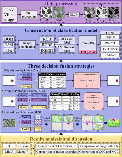
• We constructed three UAV image datasets by combing DOM, DSM, and TFs to explore the impact of different feature combinations on karst wetland vegetation mapping.
• We constructed several OCC and MCC models based on four CNN algorithms (SegNet, PSPNet, DeepLabV3+, and RAUNet) and compared the classification results of OCC and MCC models to demonstrate the advantages of OCC for classifying karst wetland vegetation communities.
• We used three decision fusion strategies (Majority Voting Fusion, Average Probability Fusion, and Optimal Selection Fusion) to fuse multiple OCC and MCC models, respectively, and evaluated the identification abilities of one-class FCMs and multi-class FCMs to demonstrate the advantages of multiple OCC models’ fusion for karst wetland vegetation mapping.
• We compared the differences in classification accuracy between FCMs and single CNN models to evaluate the effects of different decision fusion strategies on the classification of karst wetland vegetation.

2. Materials and Methods

2.1. Study Area

Huixian Karst National Wetland Park (HKNWP), Guilin, south China, is located in the core of the East Asian Karst Region, the third largest karst concentration area in the world, with a geographical location of 25°01′30″N–25°11′15″N and 110°08′15″E–110°18′00″E (as shown in Figure 1). The total area of HKNWP is 586.75 hectares, of which 84.12% (493.59 hectares) is wetland, which is the most representative and complete karst wetland in China and even in Asia [40]. The Huixian Wetland, known as the “Kidney of the Lijiang River”, is the largest original karst landscape wetland in the Lijiang River basin and has important environmental regulation functions and ecological benefits, such as water conservation, water purification, flood storage, drought resistance, and maintenance of biodiversity, and thus has high research and protection value. However, in the last half-century, with the deterioration of the ecological environment and the intensification of human activities, the ecosystem of the Huixian Wetland has been severely damaged, so the Chinese government listed it as a pilot national wetland park for conservation work in 2012 and it officially became a national wetland park in China in 2017. The HKNWP has been divided into five different areas, among which the core area is less disturbed by anthropogenic activities and still preserves a relatively complete ecological landscape of karst wetlands, which plays an important role in the study and protection of Huixian karst wetlands and is the reason for choosing it as the study area in this research.

2.2. Data Source

2.2.1. UAV Data Acquisition and Processing

The UAV aerial data were collected by the DJI Phantom 4 Pro, which has an integrated FC6310S sensor to acquire visible images. Aerial photography was conducted from 10:30 am to 15:00 am (UTM + 8:00) on 26–28 August 2020 in clear and cloudless weather with a total of 12 flights. The flight altitudes were 90 m and 40 m (40 m was the flight altitude of the sample strip) and the overlap rates of heading and side directions were 80% and 75%, respectively. The processing process of UAV images was as follows: (1) We imported the original UAV aerial images into Pix4D mapper software for automated processing, which includes quality inspection, image matching, aerial triangulation, point cloud generation, etc., and finally generated DOM and DSM with a spatial resolution of 0.05 m; (2) we used ArcGIS 10.6 software to resample the DOM and DSM to a 0.1 m spatial resolution and performed georeferencing, and the projected coordinate system was WGS 1984 UTM Zone 49N; and (3) we converted the DOM to gray image using ENVI 5.6 software and then calculated its TFs (mean, variance, homogeneity, contrast, dissimilarity, entropy, angular second moment, and correlation), after which mean, contrast, and entropy were selected by high-correlation rejection and feature selection for a total of three texture features, where the processing window was 9 × 9, the co-occurrence shift was (x, y) = (1, 1), and the greyscale quantization level was 64. Finally, we combined DOM, DSM, and TFs to obtain three image feature datasets (RGB, RGBS, and RGBST), and the detailed feature composition information is shown in

Table 1. Different image datasets.

Image Datasets	Combination	Descriptions
RGB	DOM	Blue, Green, and Red
RGBS	DOM + DSM	Blue, Green, Red, and DSM
RGBST	DOM + DSM + TFs	Blue, Green, Red, DSM, Mean, Contrast, and Entropy

.

2.2.2. Field Investigation and Semantic Label Creation

The field investigation was divided into two time periods: 26 to 28 August 2020 and 14 to 21 October 2021. We investigated the vegetation on the ground by setting a quadrat of 1 m × 1 m and used Hi-Target’s V90 GNSS RTK System to record the specific coordinates of the sample points, while the iHand55 Handheld Controller was used to photograph each square from multiple angles and record the vegetation types in the quadrat area. According to the ground investigation, the vegetation types in the aerial photography area were mainly divided into seven types of features: Karst Rivers and Lakes (KRL), Karst Herbages (KH), Paddy Field (PF), Karst Woody Plants (KWP), Eichhornia Crassipes (EC), Nelumbo Nucifera (NN), and Bare Soil and Artifacts (BSA). A total of 240 sample points were obtained, and the specific distribution is shown in Figure 2. In this research, we combined the sample data from the field investigation with the aerial strip images taken by the UAV to visually interpret the DOM using ArcGIS software, mapped the corresponding vectorized data labels, and finally generated the required semantic labels (the image size is 4603 × 3017) by vector conversion raster. The final number of verification samples and pixels is shown in

Table 2. Number of sample points and pixels for accuracy assessments.

Classes	KRL	KH	PF	KWP	EC	NN	BSA	Total
Number of samples	50	45	15	55	35	25	15	240
Number of pixels	3,508,776	3,177,450	530,202	4,420,458	1,592,524	591,233	94,083	13,887,251

.

Since the focus of this paper is on karst wetland vegetation, we grouped all land cover types except the four karst wetland vegetation types into one category (Others). This allowed us to reduce the training cost of the multiclass classification model, make it easier to fit, and focus more on the differences in classification results between different karst wetland vegetation in the subsequent quantitative and qualitative analyses, excluding the influence of other non-vegetation types.

2.3. Methods

In this paper, we created three UAV image datasets to evaluate the impact of multi-dimensional data on the classification of karst wetland vegetation. Then, we constructed different OCC and MCC models based on four CNN algorithms to compare the classification performances of wetland vegetation between OCC and MCC models. This paper further evaluated the accuracy differences of CNN-based fusion classification models (FCMs) between four deep learning algorithms in wetland vegetation classification. We constructed different one-class FCMs and multi-class FCMs and compared the identification ability of OC-FCM and MC-FCM for wetland vegetation mapping. Finally, we compared the classification performances of FCMs and the single-CNN model to examine the effectiveness of three decision fusions for classifying wetland vegetation. The technical route of this paper is shown in Figure 3.

2.3.1. CNNs-Based Wetland Vegetation Classification

SegNet [41] is a pixel-wise image semantic segmentation algorithm whose structure consists of an encoder and a decoder (Figure 4). The encoder uses the first 13 layers of the VGG-16 network and performs five iterations of double downsampling, while the decoder performs five iterations of double upsampling, showing a symmetric relationship between the two. The main contribution of this network is to guide the decoder to perform nonlinear upsampling with the pooling index in the encoder for more efficient and accurate image segmentation.

The network structure of PSPNet [42] is shown in Figure 5. The network adopts the Dilated ResNet in the DeepLab algorithm as the backbone network so that the sampling coefficient output by the encoder is 1/8 of the input image to ensure a higher-resolution feature map and improve the segmentation performance of the algorithm. The network adds a spatial pyramid pooling module after the backbone network to obtain the multi-scale features of the target through four different pooling methods, all of which use bilinear interpolation to upsample to 1/8 of the original image and fuse with the output of the backbone network. In the decoding part, bilinear upsampling is directly performed to the size of the input image to achieve image segmentation.

The network structure of DeeplabV3+ [43] is shown in Figure 6. The encoder consists of the Xception network with depthwise separable convolution and Atrous Spatial Pyramid Pooling (ASPP). The introduction of the depthwise separable convolution reduces the number of parameters without affecting the segmentation performance and the ASPP enables the algorithm to obtain multi-scale information about the target without increasing the number of parameters too much. The decoder consists of two upsampling modules, which add location information by incorporating the low-level feature output using the Xception network to obtain finer segmentation results.

The network structure of RAUNet [44] is shown in Figure 7. The encoder consists of the ResNet-34 and the decoder consists of multiple layers of the Attention Augmentation Module (AAM) and deconvolution to fuse multiple layers of target features. Among them, AAM is used to reconstruct semantic correlations and guide low-level information with high-level semantic information to emphasize key features and filter background information. Furthermore, deconvolution is used in the decoder for upsampling to obtain more refined edge features.

2.3.2. One-Class and Multi-Class Classification Models of Karst Wetland Vegetation Using CNN Algorithms and UAV Images

In this research, we used three image datasets (RGB, RGBS, and RGBST) and four CNN algorithms (SegNet, PSPNet, DeepLabV3+, and RAUNet) to construct twenty-four OCC (12) and MCC (12) models for karst wetland vegetation, which were divided into eight groups, with each group containing three classification scenarios. Among them, each scenario in groups I–IV constructs four OCC models for karst wetland vegetation (corresponding to four types of wetland vegetation, KH, KWP, EC, and NN), while each scenario in groups V–VIII constructs different MCC models for karst wetland vegetation. The details are shown in

Table 3. Construction of OCC and MCC models for karst wetland vegetation.

Models	Groups	Algorithms	Image Datasets	Scenarios
One-class classification	I	SegNet	RGB	1
			RGBS	2
			RGBST	3
	II	PSPNet	RGB	4
			RGBS	5
			RGBST	6
	III	DeepLabV3+	RGB	7
			RGBS	8
			RGBST	9
	IV	RAUNet	RGB	10
			RGBS	11
			RGBST	12
Multi-class classification	V	SegNet	RGB	13
			RGBS	14
			RGBST	15
	VI	PSPNet	RGB	16
			RGBS	17
			RGBST	18
	VII	DeepLabV3+	RGB	19
			RGBS	20
			RGBST	21
	VIII	RAUNet	RGB	22
			RGBS	23
			RGBST	24

below.

Firstly, this paper quantitatively evaluated the difference in the classification accuracy of karst wetland vegetation between different image datasets under identical CNN algorithms to explore the identification ability of different image datasets for karst wetland vegetation. Taking the SegNet algorithm and KH as an example, we compared the results of scenarios 1–3 in group I to explore the effect of the addition of DSM and TFs on the classification performance of KH. Secondly, this paper compared the differences in the classification accuracy of karst wetland vegetation of OCC models composed of different CNN algorithms combined with an identical image dataset to evaluate the impact of different CNN algorithms on the classification effect of karst wetland vegetation. Taking the RGBST image dataset and NN as an example, we compared the results of scenarios 3, 6, 9, and 12 to explore the differences in the classification performance of SegNet, PSPNet, DeepLabV3+, and RAUNet algorithms for NN. Finally, this paper compared the classification accuracy of karst wetland vegetation of OCC and MCC models based on an identical image dataset and the CNN algorithm to evaluate the difference in classification accuracy between OCC and MCC models for karst wetland vegetation. Taking the PSPNet algorithm, RGBS image dataset, and KWP as examples, we compared the results of scenarios 5 and 17 to explore the difference in the classification performance for KWP of the OCC and MCC models composed of the PSPNet algorithm combined with the RGBS image dataset.

In this research, all models were trained in a consistent manner. For the training dataset, the images of the study area were divided in a ratio of 3:1. Image data with a ratio of 3 were randomly cropped to 256 × 256 pixels and enhanced (flipped, rotated, channel exchange, etc.) to generate a dataset of 100,000 images. Of these, 80% were used as training data and the remaining 20% were validation data, and the final image data with a ratio of 1 were used as the final test data. For model optimization, the weighted cross-entropy loss function was used to guide model training to alleviate the class imbalance, where the weights were calculated using the “balance” method provided by the scikit-learn library and the Adam algorithm was used as the optimizer (learning rate = 0.001, and betas = (0.9, 0.999)) to update the model parameters to minimize the loss function. The training epoch of all models was 10, and the best model in each model period was selected for subsequent vegetation classification and accuracy assessment after the training was completed. The specific training curves for each model are shown in Figure A1, Figure A2, Figure A3, Figure A4 and Figure A5.

2.3.3. Fusion Classification Models Based on Three Fusion Strategies

This paper adopted three decision-level fusion strategies to fuse OCC and MCC models, respectively, to construct different one-class fusion classification models (OC-FCM) and multi-class fusion classification models (MC-FCM), and then quantitatively evaluated the performance of OC-FCM and MC-FCM for karst wetland vegetation.

Majority Voting Fusion (MVF) [45] The specific fusion method of this strategy is shown in Equation (1). Taking a single pixel point as an example, we first calculated the values ($X_n, n=1, \dots , 5$) of the prediction results of all the models used for fusion for that pixel point, up to a total of five types (four vegetation types and one background). After that, we counted the number of occurrences ($Count$) of different values and used the class corresponding to the value with the highest number of occurrences as the final output result ($X_{\begin{array}{c}max\\ index\end{array}}$) for that pixel. Finally, we completed the prediction of the whole image in a pixel-by-pixel manner. Taking the OCC model and EC as an example, we fused the models of scenarios 1, 4, 7, and 10 in Table 3 to obtain the OC-FCM based on the RGB image dataset to identify EC. The specific fusion process of the MVF strategy is shown in Figure 8.

$$\begin{array}{c}Prediction=X_{\begin{array}{c}max\\ index\end{array}}\left(Count\left(X_1\right),Count\left(X_2\right),\dots ,Count\left(X_n\right)\right)\end{array}$$

(1)

Average Probability Fusion (APF) [45] The specific fusion method of this strategy is shown in Equation (2). Taking a single pixel as an example, firstly, we calculated the probability distributions ($\left[P_1,P_2,\dots ,P_n\right],n=1,2,\dots ,5$) of the prediction results of all models used in fusion for that pixel; after that, we added all the probability distributions and averaged them (${\sum }_{j=0}\left[P_1,P_2,\dots ,P_n\right]/j$); then, we selected the class corresponding to the highest probability in the probability distribution as the output result ($X_{\begin{array}{c}max\\ index\end{array}}$); finally, we performed the prediction of the whole image in a pixel-by-pixel manner. Taking the OCC model and KH as an example, the models of all scenarios in Group I in Table 3 were fused to obtain the OC-FCM based on the SegNet algorithm to identify KH. The specific fusion process of the APF strategy is shown in Figure 9.

$$Prediction=X_{\begin{array}{c}max\\ index\end{array}}\left(\frac{{\sum }_{j=0}\left[P_1,P_2,\dots ,P_n\right]}{j}\right)$$

(2)

Optimal Selection Fusion (OSF) This strategy is different from the above two strategies in terms of fusion. First, we directly obtained the classification result map of all models used in the fusion and calculated the classification accuracy of each type of karst wetland vegetation in the classification results of each model. After that, we calculate the classification accuracy of the four vegetation types and selected the classification results of the model with the best accuracy for each vegetation type. Finally, we overlaid the single distribution maps of the four vegetation types to obtain the final image prediction results. When overlaying multiple classes, we covered them from top to bottom in order of accuracy, from small to large, to ensure that the pixels of the low-precision class were not overlapped by the high-precision class, further reducing the accuracy of the low-precision class. The specific fusion process of the OSF strategy is shown in Figure 10.

2.3.4. Accuracy Assessment

This paper evaluated the performance of classification models for karst wetland vegetation through the normalized confusion matrix and five precision metrics (precision, recall, F1-score, macro-average F1-score (Macro-F1), Intersection over Union (IoU), and Mean Intersection over Union (MIoU)), and the computational equations are shown in (3) to (8). The F1-score was calculated by the precision and recall in this paper. Meanwhile, the classification results were evaluated at both pixel and attribute levels. In the attribute-level assessment approach, we used the F1-score to evaluate the identification ability of each model for attribute information of a single karst wetland vegetation, and we used Macro-F1 to evaluate the identification ability of each model for overall attribute information of the four vegetation types. In the pixel-wise assessment approach, we selected IoU and MIoU to evaluate the fit between the classification results of the models and the semantic labels, where IoU was used to evaluate the identification ability of each model for the geometric information of a single karst wetland vegetation area, and MIoU was used to evaluate the identification ability of each model for the overall geometric information of the four vegetation types.

$$Precision=\frac{TP}{TP+FP}$$

(3)

$$Recall=\frac{TP}{TP+FN}$$

(4)

$$F1-score=2·\frac{Precision·Recall}{Precision+Recall}$$

(5)

$$Macro-F1=\frac{{\sum }_{i=1}^{n}F1-score}{n}$$

(6)

$$IoU=\frac{TP}{TP+FP+FN}$$

(7)

$$MIoU=\frac{{\sum }_{i=1}^{n}IoU}{n}$$

(8)

In the above equation, TP presents the number of correct classifications of vegetation types, while FP and FN are the numbers of classification errors of vegetation types. Taking Karst Herbages (KH) as an example, TP is the total number of samples/pixels that are classified as KH, FP is the total number of samples/pixels of other vegetation types that are misclassified as KH, and FN presents the total number of samples/pixels of KH that are misclassified as other vegetation types.

3. Results

3.1. One-Class and Multi-Class Classifications Based on CNN Models

This paper explored the distribution of classification accuracy metrics (IoU and F1-score) of one-class CNN (OCC) and multi-class CNN (MCC) models (Figure 11) to quantitatively analyze the difference in accuracy between OCC and MCC models. By comparing the average values of accuracy, it could be seen that for identical vegetation types, the accuracy of OCC models was higher than that of MCC models and the differences between the average values of IoU and the F1-score of the two were 3.24–10.97% and 0.65–3.78%, respectively. These results showed that OCC models had better performance for karst wetland vegetation than MCC models, and the difference between the average value of IoU of the two for KH is the largest at the pixel level, while the difference between the average value of the F1-score of the two for KWP is the largest at the attribute level.

This paper calculated the difference value of accuracy (IoU and F1-score) between OCC and MCC models at the pixel and attribute levels (Figure 12), respectively (the difference value was calculated as the accuracy of the OCC model minus that of the MCC model), to further analyze the difference in performance between the two under identical conditions for karst wetland vegetation. From Figure 12, it cn be seen that there were some differences in the classification accuracy variations of the four vegetation types, while the performance of the OCC model was better in most cases compared to the MCC model. Taking EC as an example, excluding the case of using the RGB image dataset combined with the SegNet algorithm, the difference values of IoU were greater than 0 and the difference in performance between OCC and MCC models was the largest when using the RGB image dataset combined with the RAUNet algorithm (the difference value of IoU was 6.27%). Excluding three cases (RGB_SegNet, RGBS_SegNet, and RGBS_RAUNet), the difference values of the F1-score were greater than 0, and the difference in identification ability between OCC and MCC models was greatest when using the RGB image dataset combined with the RAUNet algorithm (the difference value of the F1-score was 11.1%). The above results demonstrated that, in most cases, the OCC model was better than the MCC model in the identification ability of EC at both the pixel and attribute levels.

This paper examined the accuracy (IoU and F1-score) of OCC models for each karst wetland vegetation (Figure 13) to evaluate the differences in performance between OCC models. From Figure 13, it can be seen that there were some differences in the variation trends of accuracy between OCC models for the four types of vegetation. For KH, the values of IoU ranged from 0.3591 to 0.6494 (the value of IoU was maximized using the RGBS image dataset and PSPNet algorithm), while the values of the F1-score ranged from 0.5634 to 0.9348 (the value of F1-score was maximized using the RGBST image dataset and SegNet algorithm). For KWP, the minimum and maximum values of IoU were 0.5541 (using RGB image dataset and DeepLabV3+ algorithm) and 0.7089, respectively, while the maximum and minimum values of the F1-score were 0.8780 (using RGB image dataset and SegNet algorithm) and 1, respectively. For EC, the RGBS image dataset combined with the SegNet algorithm achieved the lowest values of IoU and F1-scores, which were 0.7053 and 0.8642, respectively; and the RGB image dataset combined with the RAUNet algorithm achieved the highest values of IoU and F1-scores, which were 0.8316 and 0.9722, respectively. For NN, the values of the F1-score were 1 for all models, while the SegNet algorithm combined with RGBS and RGB image datasets resulted in the minimum (0.9540) and maximum (0.9830) values of IoU, respectively. The above results showed that among the four types of karst wetland vegetation, NN had the most stable variation in accuracy and always had the highest classification accuracy among the two assessment methods, while KH had a larger variation in accuracy and always had the lowest classification accuracy among the two assessment methods. The reason could be that there were differences in the distribution range of different vegetation types, among which the distribution range of NN was the most concentrated and easiest to distinguish.

3.2. Fusion of CNN-Based Classification

Table 4. Differences in accuracy between OC-FCM and MC-FCM based on different image datasets.

Strategies	Models	Image Datasets
		RGB	RGBS	RGBST
		Macro-F1/MIoU	Macro-F1/MIoU	Macro-F1/MIoU
MVF	OC-FCM	0.8949/0.6965	0.9595/0.7788	0.9684/0.7653
	MC-FCM	0.9340/0.6882	0.9463/0.6949	0.9433/0.7119
APF	OC-FCM	0.9070/0.7063	0.9650/0.7864	0.9684/0.7751
	MC-FCM	0.9114/0.6712	0.9161/0.6782	0.9335/0.6970
OSF	OC-FCM	0.9039/0.7185	0.9640/0.7894	0.9390/0.7630
	MC-FCM	0.9255/0.6903	0.9287/0.7017	0.9339/0.7269

shows the difference in accuracy (Macro-F1 and MIoU) of the results of one-class fusion classification models (OC-FCMs) and multi-class fusion classification models (MC-FCMs) based on different image datasets and fusion strategies. Observing the variation of MIoU, it could be seen that under identical conditions (using identical image datasets and fusion strategies), OC-FCM achieved higher MIoU values compared to MC-FCM, and the difference in MIoU between the two was 0.83–10.82%, where OC-FCM using the RGBS image dataset and OSF strategy achieved the highest MIoU of 0.7894. These results proved that OC-FCM had better performance at the pixel level than MC-FCM for karst wetland vegetation under identical conditions, and OC-FCM using the RGBS image dataset and OSF strategy had the best performance at the pixel level. Moreover, except for the case of using the RGB image dataset, the Macro-F1 of OC-FCM in other cases was higher than that of MC-FCM under identical conditions (the difference in Macro-F1 between the two was 0.51–4.89%), and OC-FCM using the RGBST image dataset combined with the MVF or APF strategy achieved the highest Macro-F1 of 0.9684. These results proved that OC-FCM outperformed MC-FCM in classifying karst wetland vegetation at the attribute level in most cases, and OC-FCM using the RGBST image dataset combined with the MVF or APF strategy had the best performance at the attribute level. When using an identical fusion strategy, the FCMs based on the RGB image dataset achieved the lowest accuracy (MIoU and Macro-F1), and the differences between their accuracy and that of FCMs based on the RGBS and RGBST image datasets were 0.32–7.35% (MIoU) and 0.67–8.23% (Macro-F1). These results proved that FCM based on the RGB image dataset had the lowest performance at both pixel and attribute levels for karst wetland vegetation.

The results of OC-FCM and MC-FCM based on different image datasets and fusion strategies are shown in Figure 14. It can be seen that with the change in image datasets, different fusion strategies and the difference between the models used for fusion created a certain gap between the results of different FCMs.

For the results of OC-FCM (Figure 14a), when using the RGB image dataset, a large number of KH were misclassified, while the misclassification rate with the OSF strategy was slightly lower than that based on the MVF and APF strategies. When using the RGBS and RGBST image datasets, the misclassification rate was significantly lower than that based on the RGB image dataset, and the misclassification rate using the OSF strategy was slightly lower than that based on the MVF and APF strategies. These results proved that OC-FCMs based on the RGBS and RGBST image datasets had better performance for karst wetland vegetation compared with the RGB image datasets, and among the three fusion strategies, OC-FCMs based on the OSF strategy had the best performance.

For the results of MC-FCM (Figure 14b), when using the RGB image dataset, similar to OC-FCM, a large number of KH were misclassified, and the highest misclassification rate was observed when using the APF strategy from a visual point of view. When using the RGBS image dataset, the misclassification rate was visually unchanged compared with the RGB image dataset, while the misclassification rate when using the APF strategy was still the highest and the misclassification rate of MC-FCM was higher than that of OC-FCM when using the MVF and APF strategies. When using the RGBST image dataset, the misclassification rate showed a significant decrease compared with that when using the RGB and RGBS image datasets, while the misclassification rate of MC-FCM was still significantly higher than that of OC-FCM when using the MVF and APF strategies. These results proved that MC-FCM based on the RGBST image dataset had the best effect on karst wetland vegetation in the three image datasets, and the effect of MC-FCM based on the OSF strategy achieved the best result compared with MC-FCM using the MVF and APF strategies. Moreover, the effect of OC-FCM was better than that of MC-FCM under identical conditions.

Figure 15 shows the normalized confusion matrix of OC-FCM based on different image datasets at the attribute level (Figure 15a) and compares the differences in the accuracy (IoU) between OC-FCMs at the pixel level (Figure 15b). When using the RGB image dataset, it can be seen by observing the confusion matrix that the variation of recall to KH was larger among the four vegetation types, with KH achieving the highest recall when the OSF strategy was used, which was consistent with the variation trend of the corresponding IoU. When using the RGBS image dataset, it could be seen by comparing the confusion matrix that the recall of KH was improved compared with that when using the RGB image dataset, and the recall of KH remained highest when using the OSF strategy, and this phenomenon was also reflected in the variation of the corresponding IoU. When using the RGBST image dataset, the recall of KH was reduced compared with that when using the RGBS image dataset, yet it was still higher than that when using the RGB image dataset, where OC-FCM based on the OSF strategy still had the best identification ability for KH and the variation trend of the confusion matrix was also consistent with the change in IoU. The above results proved that OC-FCM based on the RGBS image dataset and the OSF strategy had the best performance for KH, both at the pixel and attribute levels. For the other three vegetation types, excluding KH, although the confusion matrix based on the attribute level did not change much, the variation trend of IoU was larger for KWP and EC in the pixel-level evaluation, except for NN. Among them, the variation trend of accuracy (IoU) of KWP was very similar to that of KH (the RGBS image dataset combined with the OSF strategy achieved the highest IoU, that is, the performance at the pixel level was optimal), while the RGB image dataset combined with the APF strategy resulted in the highest IoU of EC, that is, the optimal pixel-level classification performance was achieved.

This paper examined the difference in accuracy (F1-score and IoU) between OC-FCM and MC-FCM for each vegetation type (the difference was calculated by subtracting the F1-score/IoU of MC-FCM from the F1-score/IoU of OC-FCM) to quantitatively evaluate the difference in the effect of the two for different karst wetland vegetation when using identical image datasets (Figure 16):

• For KH, the difference values of IoU and F1-score were both greater than 0 when using the RGBS image dataset. Among them, the RGBS image dataset combined with the APF strategy resulted in the difference values of IoU and F1-score both reaching the maximum, which are 22.09% and 8.41%, respectively, while the RGB image dataset combined with the MVF strategy resulted in the difference values of IoU and F1-score both reaching the minimum, which are −10.99% and −21.71%, respectively. These results proved that the identification ability of OC-FCM for KH was better than that of MC-FCM when using the RGBS image dataset, and the difference between the identification ability of the two at the pixel level reached the maximum when using the APF strategy. Meanwhile, the RGB image dataset combined with the MVF strategy resulted in the identification ability of MC-FCM for KH surpassing that of OC-FCM.
• For KWP, the difference values of IoU and F1-score were both greater than 0 in all cases, and the RGBS image dataset combined with the APF strategy still resulted in the difference values of IoU and F1-score both reaching the maximum of 16.88% and 6.62%, respectively. These results proved that the identification ability of OC-FCM for KWP was better than that of MC-FCM, and the difference between the two reached the maximum when using the RGBS image dataset and the APF strategy.
• For EC, the difference values of IoU and F1-score were both greater than 0 when using the RGB image dataset, and the RGB image dataset combined with the APF and MVF strategies resulted in the difference values of IoU and F1-score both reaching their maximum of 3.31% and 5.22%, respectively. Meanwhile, the RGBST image dataset combined with the OSF strategy resulted in the difference values of IoU and F1-score reaching their minimum of −3.9% and −0.15%, respectively. These results proved that the identification ability of OC-FCM for EC was better than that of MC-FCM when using the RGB image dataset, and the difference in the identification abilities of the two at the pixel and attribute levels reached the maximum when using the APF and MVF strategies, respectively. Meanwhile, the identification ability of MC-FCM for EC was better than that of OC-FCM when using the RGBST image dataset and the OSF strategy.
• For NN, similar to KWP, the difference value of IoU was greater than 0 in all cases, where the RGB image dataset combined with the MVF strategy exhibited the largest difference value of IoU (6.42%), while the RGBS image dataset combined with both the MVF and APF strategies exhibited the largest difference value of F1-score (1.96%). These results proved that OC-FCM outperformed MC-FCM in identifying NN at the pixel level, and the difference in the identification ability between the two at the pixel level reached the maximum when using the RGB image dataset and the MVF strategy. Meanwhile, OC-FCM outperformed MC-FCM in identifying NN at the attribute level when using the RGBS image dataset and the MVF and APF strategies.

3.3. Fusion of Different Images Datasets Classifications

Table 5. Accuracy differences between OC-FCM and MC-FCM based on different CNN algorithms.

Strategies	Models	Algorithms
		SegNet	PSPNet	DeepLabV3+	RAUNet
		Macro-F1/MIoU	Macro-F1/MIoU	Macro-F1/MIoU	Macro-F1/MIoU
MVF	OC-FCM	0.9516/0.7490	0.9595/0.7872	0.9604/0.7592	0.9337/0.7521
	MC-FCM	0.9184/0.6692	0.9287/0.7107	0.9350/0.6758	0.9329/0.6894
APF	OC-FCM	0.9617/0.7498	0.9613/0.7862	0.9597/0.7605	0.9432/0.7539
	MC-FCM	0.9158/0.6556	0.9314/0.7091	0.9480/0.6748	0.9411/0.6804
OSF	OC-FCM	0.9685/0.7630	0.9640/0.7894	0.9496/0.7545	0.9380/0.7753
	MC-FCM	0.9344/0.6748	0.9384/0.7112	0.9451/0.6965	0.9112/0.7087

compared the accuracy (Macro-F1 and MIoU) differences between the results of OC-FCM and MC-FCM based on different CNN algorithms and fusion strategies. Similar to those based on the image dataset, the Macro-F1 and MIoU of OC-FCM were higher than those of MC-FCM under identical conditions, with the highest MIoU of 0.7894 (the PSPNet algorithm combined with the OSF strategy) and the highest Macro-F1 of 0.9496 (the DeepLabV3+ algorithm combined with the OSF strategy). These results prove that OC-FCM was better than MC-FCM regarding the identification ability for karst wetland vegetation at the pixel and attribute levels under identical conditions, and OC-FCM using the OSF strategy combined with the PSPNet and DeepLabV3+ algorithms achieved the best performance at both the pixel and attribute levels. For the four CNN algorithms, the MIoU of FCMs based on the PSPNet algorithm was higher than that of FCMs based on the other three algorithms under identical conditions, with a difference of 0.25–5.34%. Excluding the case of OC-FCM using the APF and OSF strategies combined with the SegNet and PSPNet algorithms, the Macro-F1 of FCMs based on the DeepLabV3+ algorithm was higher than that of FCMs based on the other three algorithms under identical conditions, with a difference of 0.09–3.39%. These results proved that FCMs based on the PSPNet and DeepLabV3+ algorithms achieved the optimal identification ability for karst wetland vegetation at both the pixel and attribute levels, respectively.

The results of OC-FCM and MC-FCM based on different CNN algorithms and fusion strategies are shown in Figure 17. It can be seen that there were some differences between the results of FCMs under different conditions.

For the results of the OC-FCM (Figure 17a), when using identical algorithms, the results based on the OSF strategy had the lowest misclassification rate among the three fusion strategies, while the results based on the MVF and APF strategies exhibited similar misclassification rates. When using the identical fusion strategy, the results based on the PSPNet algorithm had the lowest misclassification rate among the four CNN algorithms, and the misclassification phenomenon of KH in the results based on the other algorithms was aggravated to different degrees compared with the results based on the PSPNet algorithm. Moreover, in the OC-FCMs based on the CNN algorithm, it could be seen from the visual effect that the result of the OC-FCM using the PSPNet algorithm combined with the OSF fusion strategy had the lowest misclassification rate. These results proved that the OC-FCM based on the OSF strategy had better identification ability for karst wetland vegetation than the OC-FCM using the MVF and APF strategies, and the OC-FCM based on the PSPNet algorithm had the best performance compared with the other three algorithms. Therefore, the PSPNet algorithm combined with the OSF strategy resulted in the OC-FCM obtaining the best performance for karst wetland vegetation.

For the results of the MC-FCM (Figure 17b), when using the identical algorithm, similar to the OC-FCM, the misclassification rate based on the OSF strategy was lower compared to that when using the other two fusion strategies, while the results based on the MVF strategy showed a lower misclassification rate compared to the results using the APF strategy. When using the identical fusion strategy, similar to OC-FCM, the misclassification rate based on the PSPNet algorithm was lower than that using the other three algorithms, while the misclassification rate based on the SegNet algorithm was the highest among the four algorithms. These results proved that for the three fusion strategies, the identification ability of MC-FCM was ranked from strong to weak as follows: OSF > MVF > APF; among the four CNN algorithms, the MC-FCM based on the PSPNet algorithm had the best performance, while the MC-FCM based on the SegNet algorithm had the weakest performance. Moreover, by comparing the results of the OC-FCM and the MC-FCM under the same conditions, it could be seen that the misclassification rate of the former was lower than that of the latter, which proved that the MC-FCM was weaker than the OC-FCM in the identification ability for karst wetland vegetation under the same conditions.

Figure 18 shows the normalized confusion matrix for the results of OC-FCM based on different CNN algorithms (Figure 18a) at the attribute level while comparing the accuracy (IoU) differences for each vegetation type (Figure 18b) at the pixel level.

Under the conditions of using identical algorithms, by observing the change in IoU (Figure 18b), it could be seen that for the four algorithms, the absolute difference value of IoU for the identical vegetation when using the MVF and APF strategies was less than 1%. Meanwhile, the IoU for the karst wetland vegetation using the OSF strategy had some differences from that using the MVF and APF strategies. Taking KH and EC as examples, regardless of which algorithm was used, the IoU for KH when using the OSF strategy was higher than that for KH when using the other, which was consistent with the changes in the confusion matrix (Figure 18a), where the PSPNet algorithm combined with the OSF strategy resulted in the IoU of KH reaching the highest value at 0.6494. When using the OSF strategy, the IoU for EC was lower than that for EC using other fusion strategies, where the SegNet algorithm combined with the OSF fusion strategy resulted in the IoU of EC reaching the minimum of 0.7507. The above results proved that the identification ability of the OC-FCM based on the MVF and the APF strategies for karst wetland vegetation was almost equal when the algorithms were identical. Among the three fusion strategies, the OC-FCM based on the OSF strategy had better identification ability for KH, and the OSF strategy combined with the PSPNet algorithm resulted in the OC-FCM achieving the best identification ability for KH at the pixel level. Meanwhile, the OC-FCM based on the OSF strategy had the lowest identification ability for EC among the three fusion strategies, and the OSF strategy combined with the SegNet algorithm resulted in the identification ability of the OC-FCM for EC decreasing to the lowest value.

Under the conditions of using the identical fusion strategy, the accuracy of OC-FCM based on different algorithms differed for each vegetation type. Taking KWP and NN as examples, for KWP, when using the OSF strategy, the OC-FCM based on the PSPNet and DeepLabV3+ algorithms achieved the highest and lowest IoUs of 0.7344 and 0.6784, respectively, while the RAUNet algorithm combined with the MVP or APF strategy resulted in a minimal IoU of OC-FCM for KWP (Figure 18b). For NN, when using the OSF strategy, OC-FCM based on SegNet and RAUNet algorithms achieved the highest and lowest IoUs of 0.9832 and 0.9749, respectively, while the PSPNet algorithm combined with the APF strategy resulted in the smallest IoU of OC-FCM for KWP and the DeepLabV3+ algorithm combined with the MVF strategy resulted in the maximal IoU of OC-FCM for KWP (Figure 18b). The above results proved that the OC-FCM based on the PSPNet algorithm and the OSF strategy had the best identification ability for KWP at the pixel level, while the OC-FCM based on the SegNet algorithm and the OSF strategy had the best identification ability for NN at the pixel level.

This paper calculated the difference in accuracy (IoU and F1-score) between the results of the OC-FCM and the MC-FCM for each vegetation type under the same conditions (Figure 19) to quantitatively evaluate the difference in performance between the OC-FCM and the MC-FCM for different karst wetland vegetation when using identical algorithms:

• For KH, the difference values of IoU were all greater than 0, while the difference values of the F1-score were also greater than 0 when using the SegNet and PSPNet algorithms. Among them, the SegNet algorithm combined with the OSF strategy resulted in the difference values of IoU and F1-score reaching the maximum of 18.81% and 10.36%, respectively.
• For KWP, when using the MVF and the APF strategies, the identification ability of OC-FCM was higher than that of MC-FCM, and the difference value of IoU and F1-score reached the maximum when using the SegNet algorithm and the APF strategy (the maximum difference values of IoU and F1-score were 15.11% and 5.06%, respectively).
• For EC, the variation trends of the difference values of F1-score and IoU were similar (the difference values were greater than 0), where the RAUNet algorithm combined with the OSF strategy resulted in the maximum difference values of both F1-score and IoU, which were 2.31% and 9.90%, respectively.
• For NN, the difference values of IoU were all greater than 0, and the RAUNet algorithm combined with the APF fusion strategy resulted in the difference value of IoU reaching a maximum of 8.89%; while in the attribute-level evaluation, two cases resulted in the difference value of F1-score decreasing to less than 0 (the SegNet algorithm combined with the MVF strategy and the RAUNet algorithm combined with the OSF strategy), and there were two cases where the difference value of F1-score reached a maximum of 1.96% (the RAUNet algorithm combined with the MVF or the APF strategy).

The above results proved that the OC-FCM based on identical algorithms outperformed the MC-FCM in most cases for karst wetland vegetation. For four types of karst wetland vegetation, the SegNet algorithm combined with the OSF and the APF strategies resulted in the greatest difference in performance between the OC-FCM and the MC-FCM for KH and KWP, respectively, while the RAUNet algorithm combined with the OSF and the APF strategies resulted in the greatest difference in performance between the two for EC and NN, respectively.

3.4. Fusion of CNNs-Based and Image Datasets-Based Classifications

Table 6. Accuracy differences of OC-FCM and MC-FCM based on different fusion strategies.

Strategies	Models
	OC-FCM		MC-FCM
	Macro-F1	MIoU	Macro-F1	MIoU
MVF	0.9660	0.7683	0.9441	0.6929
APF	0.9660	0.7719	0.9406	0.6892
OSF	0.9640	0.7901	0.9343	0.7271

compares the accuracy differences between the results of the OC-FCM and the MC-FCM using the three fusion strategies. It could be seen that the results of the two types of FCM differed somewhat in the use of different fusion strategies and accuracy assessments. For OC-FCM, the MIoU using the OSF strategy was the highest among those using the three fusion strategies, with a difference of 2.18% from the lowest MIoU (using the MVF strategy), while the Macro-F1 using the MVF or APF strategy achieved the highest value of 0.9660, which was 0.2% different from the lowest Macro-F1 (using the OSF strategy). For MC-FCM, similar to OC-FCM, the highest MIoU was achieved when using the OSF strategy, and the difference compared to the lowest MIoU (using the APF strategy) was 3.79%, while the highest Macro-F1 was achieved when using the MVF strategy, which was 0.98% higher than the lowest Macro-F1 (using the OSF strategy). Moreover, compared with the MC-FCM, the results of the OC-FCM had higher values of Macro-F1 and MIoU under identical conditions, which were 2.19–2.97% and 6.31–8.27% higher, respectively. The above results proved that regardless of which fusion strategy was adopted, the identification ability of OC-FCM was better than that of MC-FCM for karst wetland vegetation, among which the OC-FCM based on the OSF strategy had the best performance for karst wetland vegetation at the pixel level while the OC-FCM using three fusion strategies exhibited little difference in performance for karst wetland vegetation at the attribute level.

To explore the differences in performance between the FCMs based on different fusion strategies, we plotted the results of the OC-FCM and the MC-FCM based on three fusion strategies (Figure 20), calculated the IoU of each vegetation type (Figure 21b), and plotted the normalized confusion matrix at the attribute level (Figure 21a). For OC-FCM, the misclassification rates using the three fusion strategies were ranked from largest to smallest as follows: MVF > APF > OSF, which could be mostly attributed to the gradual improvement of KH being misclassified (observing the changes in the confusion matrix and IoU). Therefore, among the three types of OC-FCM, the best identification ability for KH was achieved when using the OSF strategy, whose IoU was 7.87% higher than the lowest identification ability (using the MVF strategy). For MC-FCM, similar to OC-FCM in terms of visual effects, the misclassification rate was the lowest when using the OSF strategy, while the difference between the misclassification rates using the MVF and APF strategies was small, which coincided with the variation trend of the corresponding confusion matrix and IoU for each vegetation type. The main reason for this difference was the variation of misclassification of KH, which was consistent with OC-FCM. Therefore, in the three types of the MC-FCM, the best identification ability for KH was also the best when using the OSF strategy, and the difference value of IoU between the best identification ability and the lowest identification ability (using the APF strategy) was 7.64%. Moreover, under identical conditions, the performance of the OC-FCM outperformed the MC-FCM for KH, KWP, and NN, while the performance of the OC-FCM was also better than that of the MC-FCM for EC, excluding the case of using the OSF strategy, and the difference in IoU between the two for each vegetation type ranged from 1.05% to 14.45%.

4. Discussion

The accuracy (Figure 11) of OCC and MCC models for karst wetland vegetation showed that the OCC and MCC models achieved average F1-score values of 92.12% and 90.03%, respectively, and the average F1-score values of OCC and MCC models for the four vegetation types were all above 77%. These results proved that high-resolution UAV visible images combined with the CNN algorithm achieved high-accuracy classification for karst wetland vegetation. From the difference in accuracy between OCC and MCC models for karst wetland vegetation under identical conditions (Figure 12), it could be seen that the difference values of IoU and F1-score between OCC and MCC models for the four types of vegetation were greater than 0 in most cases, and the mean difference values of IoU for KH, KWP, EC, and NN were 10.97%, 9.03%, 3.24%, and 5.84%, respectively. These results proved that OCC models tend to outperform MCC models for the four types of karst wetland vegetation, but there were disparities in the classification performance for different vegetation types, which may be caused by differences in the training samples of vegetation types in the study area, similar to the results of Feyisa et al. [46]. Furthermore, upon observing the difference in classification accuracy of OCC models based on different image datasets for four types of karst wetland vegetation (Figure 13), it could be seen that the IoU for KH and KWP improved by 6.69–20.75% and 5.6–13.23% when using the RGBS and the RGBST image datasets, respectively, compared with the RGB image datasets. These results proved that the addition of DSM and TF improved the classification accuracy of the CNN algorithm for karst wetland vegetation since there were certain differences in height and surface texture between different types of karst wetland vegetation. The addition of height and texture information could improve the differentiation between different vegetation types [47,48]. In future research, to further classify karst wetland vegetation in more detail, we consider using image features such as UAV multispectral and vegetation index to improve the differentiation between different vegetation types and using better algorithms (e.g., Vision Transformer) to achieve more accurate and detailed classification for karst wetland vegetation.

Due to the differences in image datasets and CNN algorithms between the models used in fusion, the performance of different FCMs was different. By observing the differences in the accuracy (Macro-F1 and MIoU) of FCMs using different image datasets (Table 4), we showed that Macro-F1 and MIoU of FCMs using the RGBS and RGBST image datasets were higher than those using the RGB image datasets, where the values of Macro-F1 and MIoU were higher by 0.47–7.35% and 0.67–8.23%, respectively. These results proved that the addition of DSM and TFs also improved the performance of FCM for karst wetland vegetation. By examining the accuracy (Macro-F1 and MIoU) of the results of FCMs based on different CNN algorithms (Table 5), we found that FCMs based on the PSPNet and DeepLabV3+ algorithms achieved the highest average values of MIoU and Macro-F1 of 74.89% and 94.96%, respectively. These results proved that the FCM based on the PSPNet algorithm at the pixel level had the best identification ability for karst wetland vegetation, and similarly, the FCM based on the DeepLabV3+ algorithm had the best identification ability for karst wetland vegetation at the attribute level. In addition, by examining the difference between the IoU for karst wetland vegetation after model fusion and the highest IoU before fusion (Figure 22), we found that the improvement in classification accuracy for karst wetland vegetation after model fusion varied with the adopted image dataset and CNN algorithm. Among the four types of karst wetland vegetation, the improvement of IoU for KWP was the most obvious, in which the difference in the average value of IoU before and after fusion for KWP achieved the highest value of 0.59% among the three image datasets when using the RGBS image dataset. Similarly, the difference in the average value of IoU before and after fusion for KWP achieved the highest value of 1.38% among the four algorithms when using the PSPNet algorithm. These results proved that the identification ability of the fused model for karst wetland vegetation was further improved compared to that before fusion, which has some similarities with the findings of Hoffmann et al. [49].

For model fusion, there were some differences in the classification results of the models obtained by using different fusion strategies. By comparing the visual results (Figure 15, Figure 18 and Figure 21) and the accuracy (MIoU and Macro-F1) of FCMs based on the three strategies (Table 4, Table 5 and Table 6), we found that in most cases, the classification results based on the OSF strategy achieved the lowest misclassification rate and the highest MIoU, respectively, where the MIoU was 0.04–2.99% higher than those based on the MVF and APF strategies. These results proved that the FCM using the OSF strategy was more suitable for the classification of karst wetland vegetation. By examining the difference between the accuracy (IoU) of the classification models based on the three fusion strategies and the best accuracy before the fusion (Figure 23), we found that the classification accuracy for KWP, EC, and NN improved to different degrees after the model fusion. Among them, the OC-FCM and MC-FCM using the OSF strategy resulted in the improvement of IoU for KWP by 2.55% and 0.27%, respectively. The MC-FCM based on three fusion strategies resulted in the improvement of IoU for EC by 0.55–1.28%, while the OC-FCM based on the MVF and APF strategies and the MC-FCM based on the OSF strategy resulted in the improvement of IoU for NN by 0.11–0.12%. These results proved that all three fusion strategies were able to improve the identification ability of the fused models for karst wetland vegetation. However, it could also be observed in Figure 23 that the accuracy (IoU) for some vegetation types decreased after fusion, especially when using the APF and MVF strategies. The reason was likely due to the fact that the classification performance of the models used in the fusion was mostly different from that of the optimal model, which caused the fused models to suffer from the influence of most of the models with poorer classification performance and reduced classification performance. In addition, by examining the IoU differences between OC-FCM and MC-FCM for karst wetland vegetation under different conditions (Figure 17, Figure 20 and Figure 22), we found that the IoU of OC-FCM was higher than that of MC-FCM for karst wetland vegetation in most cases. Among them, the enhancement of IoU of the OC-FCM compared to the MC-FCM for KH, KWP, EC, and NN ranged from 2% to 22.09%, 4.95% to 16.88%, 0.6% to 3.13%, and 0.59% to 8.89%, respectively. These results proved that the OC-FCM under the same conditions was better than the MC-FCM in identifying the four types of karst wetland vegetation in most cases.

5. Conclusions

This paper is pioneering in the evaluation of decision fusions for classifying karst wetland vegetation in Huixian Karst National Wetland Park, Guilin, south China, using one-class and multi-class CNN models with high-resolution UAV images. We demonstrated that the use of additional TFs and DSM derived from UAV aerial images improved the classification accuracies of karst wetland vegetation when compared to using only RGB images and achieved an increase in accuracy (IoU) of 20.75% for karst herbs based on one-class classification (OCC) models. We found that the OCC models outperformed multi-class classification (MCC) models for karst wetland vegetation mapping, and the highest accuracy (average value of IoU) difference was up to 10.97%. This study confirmed that fusion classification models (FCMs) have different identification abilities regarding wetland vegetation using different image datasets and CNN algorithms. The RGBS-based and RGBST-based FCMs provide better classification performances compared to the RGB image dataset-based FCMs. For the classification of different CNN algorithms via fusion, PSPNet and DeepLabV3 + achieved the highest average accuracies at the pixel scale (MIoU) and attribute scale (Macro-F1), reaching 74.89% and 94.96%, respectively, which proved that the PSPNet and DeepLabV3 + algorithms have the optimal capability in pixel-based and attribute-based classification for karst wetland vegetation, respectively. The FCMs improved the classification accuracies (IoU) for karst woody plants, Eichhornia crassipes, and Nelumbo nucifera by 0.27–2.55%, 0.55–1.28%, and 0.11–0.12%, respectively, when compared to the single CNN model, which revealed that three fusion strategies improved the classification performance of the CNN models for karst wetland vegetation. One-class FCMs produced a better classification of karst wetland vegetation than multi-class FCMs with an accuracy improvement of 0.59–22.09%.

References

1. Ford, D.; Williams, P.D. Karst Hydrogeology and Geomorphology; John Wiley & Sons: Hoboken, NJ, USA, 2013; ISBN 9781118684993. [Google Scholar]
2. Guo, F.; Jiang, G.; Yuan, D. Major Ions in Typical Subterranean Rivers and Their Anthropogenic Impacts in Southwest Karst Areas, China. Environ. Geol. 2007, 53, 533–541. [Google Scholar] [CrossRef]
3. Wang, K.; Zhang, C.; Chen, H.; Yue, Y.; Zhang, W.; Zhang, M.; Qi, X.; Fu, Z. Karst Landscapes of China: Patterns, Ecosystem Processes and Services. Landsc. Ecol. 2019, 34, 2743–2763. [Google Scholar] [CrossRef] [Green Version]
4. Wang, X.; Li, W.; Xiao, Y.; Cheng, A.; Shen, T.; Zhu, M.; Yu, L. Abundance and Diversity of Carbon-Fixing Bacterial Communities in Karst Wetland Soil Ecosystems. CATENA 2021, 204, 105418. [Google Scholar] [CrossRef]
5. Pipan, T.; Culver, D.C. Wetlands in cave and karst regions. In Encyclopedia of Caves; Elsevier: Amsterdam, The Netherlands, 2019; pp. 1156–1164. [Google Scholar]
6. Beltram, G. Karst Wetlands. In The Wetland Book; Springer: Dordrecht, The Netherlands, 2016; pp. 1–17. [Google Scholar]
7. Kokaly, R.F.; Despain, D.G.; Clark, R.N.; Livo, K.E. Mapping Vegetation in Yellowstone National Park Using Spectral Feature Analysis of AVIRIS Data. Remote Sens. Environ. 2003, 84, 437–456. [Google Scholar] [CrossRef] [Green Version]
8. Oostdijk, M.; Santos, M.J.; Whigham, D.; Verhoeven, J.; Silvestri, S. Assessing Rehabilitation of Managed Mangrove Ecosystems Using High Resolution Remote Sensing. Estuar. Coast. Shelf Sci. 2018, 211, 238–247. [Google Scholar] [CrossRef]
9. Bhatnagar, S.; Gill, L.; Regan, S.; Naughton, O.; Johnston, P.; Waldren, S.; Ghosh, B. Mapping vegetation communities inside wetlands using sentinel-2 imagery in ireland. Int. J. Appl. Earth Obs. Geoinf. 2020, 88, 102083. [Google Scholar] [CrossRef]
10. Li, N.; Lu, D.; Wu, M.; Zhang, Y.; Lu, L. Coastal Wetland Classification with Multiseasonal High-Spatial Resolution Satellite Imagery. Int. J. Remote Sens. 2018, 39, 8963–8983. [Google Scholar] [CrossRef]
11. Alvarez-Vanhard, E.; Houet, T.; Mony, C.; Lecoq, L.; Corpetti, T. Can UAVs Fill the Gap between in Situ Surveys and Satellites for Habitat Mapping? Remote Sens. Environ. 2020, 243, 111780. [Google Scholar] [CrossRef]
12. Martínez Prentice, R.; Villoslada Peciña, M.; Ward, R.D.; Bergamo, T.F.; Joyce, C.B.; Sepp, K. Machine Learning Classification and Accuracy Assessment from High-Resolution Images of Coastal Wetlands. Remote Sens. 2021, 13, 3669. [Google Scholar] [CrossRef]
13. Gray, P.; Ridge, J.; Poulin, S.; Seymour, A.; Schwantes, A.; Swenson, J.; Johnston, D. Integrating Drone Imagery into High Resolution Satellite Remote Sensing Assessments of Estuarine Environments. Remote Sens. 2018, 10, 1257. [Google Scholar] [CrossRef]
14. Pande-Chhetri, R.; Abd-Elrahman, A.; Liu, T.; Morton, J.; Wilhelm, V.L. Object-Based Classification of Wetland Vegetation Using Very High-Resolution Unmanned Air System Imagery. Eur. J. Remote Sens. 2017, 50, 564–576. [Google Scholar] [CrossRef] [Green Version]
15. Wu, N.; Shi, R.; Zhuo, W.; Zhang, C.; Tao, Z. Identification of Native and Invasive Vegetation Communities in a Tidal Flat Wetland Using Gaofen-1 Imagery. Wetlands 2021, 41, 46. [Google Scholar] [CrossRef]
16. Banks, S.; White, L.; Behnamian, A.; Chen, Z.; Montpetit, B.; Brisco, B.; Pasher, J.; Duffe, J. Wetland Classification with Multi-Angle/Temporal SAR Using Random Forests. Remote Sens. 2019, 11, 670. [Google Scholar] [CrossRef] [Green Version]
17. Deval, K.; Joshi, P.K. Vegetation Type and Land Cover Mapping in a Semi-Arid Heterogeneous Forested Wetland of India: Comparing Image Classification Algorithms. Environ. Dev. Sustain. 2021, 24, 3947–3966. [Google Scholar] [CrossRef]
18. Balogun, A.-L.; Yekeen, S.T.; Pradhan, B.; Althuwaynee, O.F. Spatio-Temporal Analysis of Oil Spill Impact and Recovery Pattern of Coastal Vegetation and Wetland Using Multispectral Satellite Landsat 8-OLI Imagery and Machine Learning Models. Remote Sens. 2020, 12, 1225. [Google Scholar] [CrossRef] [Green Version]
19. Zhang, M.; Lin, H. Wetland Classification Using Parcel-Level Ensemble Algorithm Based on Gaofen-6 Multispectral Imagery and Sentinel-1 Dataset. J. Hydrol. 2022, 606, 127462. [Google Scholar] [CrossRef]
20. Pardede, H.F.; Suryawati, E.; Krisnandi, D.; Yuwana, R.S.; Zilvan, V. Machine Learning Based Plant Diseases Detection: A Review. In Proceedings of the 2020 International Conference on Radar, Antenna, Microwave, Electronics, and Telecommunications (ICRAMET), Tangerang, Indonesia, 18–20 November 2020. [Google Scholar] [CrossRef]
21. Zhong, B.; Pan, X.; Love, P.E.D.; Ding, L.; Fang, W. Deep Learning and Network Analysis: Classifying and Visualizing Accident Narratives in Construction. Autom. Constr. 2020, 113, 103089. [Google Scholar] [CrossRef]
22. Wang, Z.; Hong, T.; Piette, M.A. Building Thermal Load Prediction through Shallow Machine Learning and Deep Learning. Appl. Energy 2020, 263, 114683. [Google Scholar] [CrossRef] [Green Version]
23. Scepanovic, S.; Antropov, O.; Laurila, P.; Rauste, Y.; Ignatenko, V.; Praks, J. Wide-Area Land Cover Mapping With Sentinel-1 Imagery Using Deep Learning Semantic Segmentation Models. IEEE J. Sel. Top. Appl. Earth Obs. Remote Sens. 2021, 14, 10357–10374. [Google Scholar] [CrossRef]
24. Lin, F.-C.; Chuang, Y.-C. Interoperability Study of Data Preprocessing for Deep Learning and High-Resolution Aerial Photographs for Forest and Vegetation Type Identification. Remote Sens. 2021, 13, 4036. [Google Scholar] [CrossRef]
25. Liu, M.; Fu, B.; Xie, S.; He, H.; Lan, F.; Li, Y.; Lou, P.; Fan, D. Comparison of Multi-Source Satellite Images for Classifying Marsh Vegetation Using DeepLabV3 Plus Deep Learning Algorithm. Ecol. Indic. 2021, 125, 107562. [Google Scholar] [CrossRef]
26. Fu, B.; He, X.; Yao, H.; Liang, Y.; Deng, T.; He, H.; Fan, D.; Lan, G.; He, W. Comparison of RFE-DL and Stacking Ensemble Learning Algorithms for Classifying Mangrove Species on UAV Multispectral Images. Int. J. Appl. Earth Obs. Geoinf. 2022, 112, 102890. [Google Scholar] [CrossRef]
27. Pashaei, M.; Kamangir, H.; Starek, M.J.; Tissot, P. Review and Evaluation of Deep Learning Architectures for Efficient Land Cover Mapping with UAS Hyper-Spatial Imagery: A Case Study Over a Wetland. Remote Sens. 2020, 12, 959. [Google Scholar] [CrossRef] [Green Version]
28. Zhao, H.; Zhong, Y.; Wang, X.; Hu, X.; Luo, C.; Boitt, M.; Piiroinen, R.; Zhang, L.; Heiskanen, J.; Pellikka, P. Mapping the Distribution of Invasive Tree Species Using Deep One-Class Classification in the Tropical Montane Landscape of Kenya. ISPRS J. Photogramm. Remote Sens. 2022, 187, 328–344. [Google Scholar] [CrossRef]
29. Lu, Y.; Wang, L. How to Automate Timely Large-Scale Mangrove Mapping with Remote Sensing. Remote Sens. Environ. 2021, 264, 112584. [Google Scholar] [CrossRef]
30. Sanjeewani, P.; Verma, B. Single Class Detection-Based Deep Learning Approach for Identification of Road Safety Attributes. Neural Comput. Appl. 2021, 33, 9691–9702. [Google Scholar] [CrossRef]
31. Tang, T.Y.; Fu, B.L.; Lou, P.Q.; Bi, L. Segnet-based extraction of wetland vegetation information from UAV images. Int. Arch. Photogramm. Remote Sens. Spat. Inf. Sci. 2020, 42, 375–380. [Google Scholar] [CrossRef] [Green Version]
32. Xiao, Y.; Wu, J.; Lin, Z.; Zhao, X. A Deep Learning-Based Multi-Model Ensemble Method for Cancer Prediction. Comput. Methods Programs Biomed. 2018, 153, 1–9. [Google Scholar] [CrossRef]
33. Choi, Y.; Chung, H.I.; Lim, C.H.; Lee, J.; Sung, H.C.; Jeon, S.W. Machine Learning Approach to Predict Vegetation Health Using Multi-Source Geospatial Data. In Proceedings of the AGU Fall Meeting 2021, New Orleans, LA, USA, 13–17 December 2021. [Google Scholar]
34. Man, C.D.; Nguyen, T.T.; Bui, H.Q.; Lasko, K.; Nguyen, T.N.T. Improvement of Land-Cover Classification over Frequently Cloud-Covered Areas Using Landsat 8 Time-Series Composites and an Ensemble of Supervised Classifiers. Int. J. Remote Sens. 2017, 39, 1243–1255. [Google Scholar] [CrossRef]
35. Hang, R.; Li, Z.; Ghamisi, P.; Hong, D.; Xia, G.; Liu, Q. Classification of Hyperspectral and LiDAR Data Using Coupled CNNs. IEEE Trans. Geosci. Remote Sens. 2020, 58, 4939–4950. [Google Scholar] [CrossRef] [Green Version]
36. Zhang, C.; Sargent, I.; Pan, X.; Gardiner, A.; Hare, J.; Atkinson, P.M. VPRS-Based Regional Decision Fusion of CNN and MRF Classifications for Very Fine Resolution Remotely Sensed Images. IEEE Trans. Geosci. Remote Sens. 2018, 56, 4507–4521. [Google Scholar] [CrossRef] [Green Version]
37. Hu, Y.; Zhang, J.; Ma, Y.; An, J.; Ren, G.; Li, X. Hyperspectral Coastal Wetland Classification Based on a Multiobject Convolutional Neural Network Model and Decision Fusion. IEEE Geosci. Remote Sens. Lett. 2019, 16, 1110–1114. [Google Scholar] [CrossRef]
38. Meng, X.; Zhang, S.; Zang, S. Lake Wetland Classification Based on an SVM-CNN Composite Classifier and High-Resolution Images Using Wudalianchi as an Example. J. Coast. Res. 2019, 93, 153. [Google Scholar] [CrossRef]
39. Deng, T.; Fu, B.; Liu, M.; He, H.; Fan, D.; Li, L.; Huang, L.; Gao, E. Comparison of Multi-Class and Fusion of Multiple Single-Class SegNet Model for Mapping Karst Wetland Vegetation Using UAV Images. Sci. Rep. 2022, 12, 13270. [Google Scholar] [CrossRef]
40. Xiao, H.; Shahab, A.; Li, J.; Xi, B.; Sun, X.; He, H.; Yu, G. Distribution, Ecological Risk Assessment and Source Identification of Heavy Metals in Surface Sediments of Huixian Karst Wetland, China. Ecotoxicol. Environ. Saf. 2019, 185, 109700. [Google Scholar] [CrossRef]
41. Badrinarayanan, V.; Kendall, A.; Cipolla, R. SegNet: A Deep Convolutional Encoder-Decoder Architecture for Image Segmentation. IEEE Trans. Pattern Anal. Mach. Intell. 2017, 39, 2481–2495. [Google Scholar] [CrossRef]
42. Zhao, H.; Shi, J.; Qi, X.; Wang, X.; Jia, J. Pyramid Scene Parsing Network. In Proceedings of the 2017 IEEE Conference on Computer Vision and Pattern Recognition (CVPR), Honolulu, HI, USA, 21–26 July 2017. [Google Scholar] [CrossRef] [Green Version]
43. Chen, L.-C.; Zhu, Y.; Papandreou, G.; Schroff, F.; Adam, H. Encoder-Decoder with Atrous Separable Convolution for Semantic Image Segmentation. In Computer Vision—ECCV 2018; Springer: Cham, Switzerland, 2018; pp. 833–851. [Google Scholar] [CrossRef] [Green Version]
44. Ni, Z.-L.; Bian, G.-B.; Zhou, X.-H.; Hou, Z.-G.; Xie, X.-L.; Wang, C.; Zhou, Y.-J.; Li, R.-Q.; Li, Z. RAUNet: Residual Attention U-Net for Semantic Segmentation of Cataract Surgical Instruments. In International Conference on Neural Information Processing; Springer: Cham, Switzerland, 2019; pp. 139–149. [Google Scholar] [CrossRef]
45. Takruri, M.; Rashad, M.W.; Attia, H. Multi-Classifier Decision Fusion for Enhancing Melanoma Recognition Accuracy. In Proceedings of the 2016 5th International Conference on Electronic Devices, Systems and Applications (ICEDSA), Ras Al Khaimah, United Arab Emirates, 6–8 December 2016. [Google Scholar] [CrossRef]
46. Feyisa, G.L.; Palao, L.K.; Nelson, A.; Gumma, M.K.; Paliwal, A.; Win, K.T.; Nge, K.H.; Johnson, D.E. Characterizing and Mapping Cropping Patterns in a Complex Agro-Ecosystem: An Iterative Participatory Mapping Procedure Using Machine Learning Algorithms and MODIS Vegetation Indices. Comput. Electron. Agric. 2020, 175, 105595. [Google Scholar] [CrossRef]
47. Hu, K.; Zhang, S.; Zhao, X. Context-Based Conditional Random Fields as Recurrent Neural Networks for Image Labeling. Multimed. Tools Appl. 2019, 79, 17135–17145. [Google Scholar] [CrossRef]
48. Al-Najjar, H.A.H.; Kalantar, B.; Pradhan, B.; Saeidi, V.; Halin, A.A.; Ueda, N.; Mansor, S. Land Cover Classification from Fused DSM and UAV Images Using Convolutional Neural Networks. Remote Sens. 2019, 11, 1461. [Google Scholar] [CrossRef] [Green Version]
49. Hoffmann, E.J.; Wang, Y.; Werner, M.; Kang, J.; Zhu, X.X. Model Fusion for Building Type Classification from Aerial and Street View Images. Remote Sens. 2019, 11, 1259. [Google Scholar] [CrossRef]
Figure 1. Geographical location of study area and field measurements.
Remotesensing 14 05869 g001
Figure 2. Semantic label and the distribution of quadrat. (a) Label, (b) DOM and sampling point.
Remotesensing 14 05869 g002
Figure 3. Technical route. It is divided into three sections from left to right. The first section on the left is the data processing of UAV images. The second section in the middle is divided into three parts: (1) Construction of image datasets; (2) training of four one- and multi-class CNN classification models. Three combination datasets of UAV images and their semantic labels were used for training of SegNet, PSPNet, DeepLabV3+, and RAUNet, respectively, and OCC and MCC models were built; (3) three decision fusion strategies, which are explained in detail in Section 2.3.3. The third section on the right is the accuracy assessment metrics and comparative analysis of classification results between different classification models.
Remotesensing 14 05869 g003
Figure 4. Structure of the SegNet algorithm.
Remotesensing 14 05869 g004
Figure 5. Structure of the PSPNet algorithm.
Remotesensing 14 05869 g005
Figure 6. Structure of the DeepLabV3+ algorithm.
Remotesensing 14 05869 g006
Figure 7. Structure of the RAUNet algorithm.
Remotesensing 14 05869 g007
Figure 8. The framework of majority voting fusion method.
Remotesensing 14 05869 g008
Figure 9. The framework of average probability fusion method.
Remotesensing 14 05869 g009
Figure 10. The framework of optimal selection fusion method.
Remotesensing 14 05869 g010
Figure 11. Statistics of accuracy of vegetation by one-class and multi-class CNN models. (a) IoU, (b) F1-score.
Remotesensing 14 05869 g011
Figure 12. The accuracy differences of IoU and F1-score between OCC and MCC models for karst wetland vegetation.
Remotesensing 14 05869 g012
Figure 13. Statistics of accuracy of OCC models for karst wetland vegetation. (a) IoU, (b) F1-score.
Remotesensing 14 05869 g013
Figure 14. Classification results for karst wetland vegetation based on different image datasets. (a) OC-FCM, (b) MC-FCM, (c) semantic label and UAV data.
Remotesensing 14 05869 g014
Figure 15. Comparison of the classification accuracies of OC-FCMs with different image datasets for karst wetland vegetation. (a) Normalized confusion matrix, (b) IoU.
Remotesensing 14 05869 g015
Figure 16. The accuracy differences between OC-FCMs and MC-FCMs with different image datasets for karst wetland vegetation.
Remotesensing 14 05869 g016
Figure 17. Results of OC-FCM and MC-FCM based on different algorithms for karst wetland vegetation. (a) OC-FCM, (b) MC-FCM, (c) semantic label and UAV data.
Remotesensing 14 05869 g017
Figure 18. Differences in accuracy of OC-FCMs based on different algorithms for karst wetland vegetation. (a) Normalized confusion matrix, (b) IoU.
Remotesensing 14 05869 g018
Figure 19. Differences in accuracy between the OC-FCM and the MC-FCM based on different algorithms for karst wetland vegetation.
Remotesensing 14 05869 g019
Figure 20. Results of the OC-FCM and MC-FCM based on different fusion strategies for karst wetland vegetation. (a) OC-FCM and MC-FCM, (b) semantic labels and UAV data.
Remotesensing 14 05869 g020
Figure 21. Differences in accuracy of the OC-FCM based on different fusion strategies for karst wetland vegetation. (a) normalized confusion matrix, (b) IoU.
Remotesensing 14 05869 g021
Figure 22. Difference between the IoU of model fusion for each karst wetland vegetation and the highest IoU before fusion. (a) FCMs based on different image datasets and (b) FCMs based on different CNN algorithms.
Remotesensing 14 05869 g022
Figure 23. Difference between the IoU of FCMs based on different strategies and the best IoU of the single CNN models before fusion for karst wetland vegetation.
Remotesensing 14 05869 g023