
HF Noise Characteristics over Cyprus


1
Frederick Research Center, 1303 Nicosia, Cyprus
2
Department of Electrical Engineering, Computer Engineering and Informatics, School of Engineering, Frederick University, 1036 Nicosia, Cyprus
*
Author to whom correspondence should be addressed.
Remote Sens. 2022, 14(23), 6040; https://doi.org/10.3390/rs14236040
Submission received: 31 October 2022
/
Revised: 24 November 2022
/
Accepted: 25 November 2022
/
Published: 29 November 2022
Abstract
:Due to the long distance propagation characteristics of the HF spectrum, noise and interference are significant and challenging factors that have to be addressed in the context of HF system performance. Both aspects exhibit systematic diurnal, seasonal, and solar cycle variability that result in a number of corresponding measurement campaigns all over the globe, in an effort to characterise HF noise. Noise at HF consists of man-made and naturally occurring HF noise with atmospheric and galactic components. An understanding of HF noise variation in terms of time, azimuth, and filter bandwidth is crucial for a specific location, as it can provide a background knowledge based on which appropriate values of HF system parameters may be selected. This paper deals with the temporal, azimuthal, and bandwidth characteristics of HF noise based on a one-month dataset of electric field strength measurements recorded by a directional antenna in Cyprus.
1. Introduction
Noise and interference from other users represent important challenges for HF (formally defined to extend from 3 to 30 MHz) communication and Over The Horizon Radar (OTHR) systems as a result of their long distance HF propagation characteristics. The temporal characteristics of both HF interference from other users and HF noise are depicted on systematic diurnal, seasonal, and solar cycle features at a certain geographic location. Various past measurement campaigns have contributed to the characterization of interference from other users [1,2]. Other experiments resulted in extended datasets, which facilitated the development of HF spectral model specifications exploiting time-series and non-linear regression modeling approaches, as well as existing ionospheric models coupled with ray-tracing [3,4,5,6,7]. Noise at HF has been the focus of extended investigation in past studies, and consists of man-made and naturally occurring HF noise with atmospheric and galactic components. The atmospheric component is driven by lightning strikes, which is the superposition of noise, propagating through line-of-sight ground waves originating from local thunderstorm activity within 100 km, and skywave noise from distant thunderstorms propagating via the ionosphere. Skywave noise results from the superposition of many lightning strikes on a global scale (170,000/h according to [8]), and exhibits diurnal, seasonal, and directional characteristics. Coleman used an accurate propagation model to improve a model by Kotaki based on the global distribution of thunderstorm activity [9,10]. The galactic component is generated by our Sun, and also arrives as cosmic radiation from other stars through transionospheric propagation. As a result, it contributes mostly at higher frequencies and high elevation angles since energy at low frequency and low elevation angles is attenuated by the ionosphere.
Based on past studies, HF noise was characterized as Gaussian [11], non-Gaussian [12,13,14] and consisting of Gaussian, impulsive, and discrete interferer components [15,16,17]. Several extended measurement campaigns have been carried out with reference to specific applications (OTHR) [18,19] and resulted in model specifications to encapsulate such features [20,21].
An understanding of the directional characteristics of HF noise is very important for practical HF systems such as OTHRs which employ highly directive antenna arrays beamed to certain orientations and are therefore particularly sensitive to the highly anisotropic HF noise environment. Such systems are also in operation in Cyprus [22]. Past studies dealt with the non-uniform azimuthal noise distribution, which is important for the understanding of HF receiver antenna signal-to-noise performance [9,21,23]. Antenna directivity is expected to affect both noise and spectral occupancy statistics. Some work has been carried out on the azimuthal distribution of noise by Gibson and Arnett, at a measurement site in southern England [24]. This showed that the greatest asymmetry in noise intensity was observed between the south-east and north-west, during 1600–2000 h UT, at frequencies near 10 MHz, during spring and summer. The results were generally consistent with the expected distribution of atmospheric noise from thunderstorm activity. The day-to-day variability of noise was found to be the greatest from the south-east. At frequencies below about 20 MHz, the noise received at a quiet rural site is predicted to be mainly of atmospheric origin [25].
Another important aspect of noise and interference from other users at HF is their dependence upon measuring filter bandwidth. Regarding interference from other users, it is established that HF channel spectral occupancy is very dependent on the measuring filter bandwidth [26]. Subsequently, there have been efforts to express this dependence using a model specification for a limited number of HF allocations, which was later extended to cover all allocations in the HF spectrum [27]. A similar work was undertaken by Andersson, who combined contiguous sample values obtained whilst using a narrow filter, enabling occupancy to be derived for a range of equivalent bandwidths instead of using different IF filter bandwidths [28].
This paper deals with the temporal, azimuthal, and bandwidth characteristics of HF noise based on a monthly campaign to assemble a dataset from electric field measurements received by a directional antenna in Cyprus.
2. HF Noise Measurements
Since the HF spectrum is subject to an international agreement on its utilization, it is divided by the International Telecommunications Union (ITU) into frequency allocations on the basis of nine different types of user. Interference characteristics for distinct types of user exhibit significant differences, therefore the dataset was divided in to 95 ITU defined frequency allocations of different user types in accordance to Table 1. This is because different user types employ different transmission powers, bandwidths, modulation schemes and operating procedures. The dataset was collected by a dedicated HF monitoring system operating in Cyprus, with the aim to facilitate measurement and analysis of specific attributes expected to affect HF noise distribution, such as frequency range, time of day, azimuth, and measurement filter bandwidth. The frequency ranges that were used in this study are highlighted in Table 1.
The measurement system is based on an R&S EM 510 digital wideband HF receiver connected to an Array-solutions SAL-12 antenna [29] which can be automatically steered through a controller (Figure 1). Each azimuthal measurement session was initiated at midnight (00:00 LT) by connecting the SAL-12 antenna steered in the north direction to the antenna input of the R&S EM 510 measurement receiver, which was able to determine the RMS field strength (in dBµV/m) using a 1 s dwell time, so that the full range of each HF spectrum allocation indicated in Table 1 could be sampled within 10 min. Then the antenna was steered by 45° to north-east and subsequently covered all eight (N-NW) 45° sectors in 80 min, resulting in 144 10-min scans, which corresponds to 18 full rotations within an allocation, capturing all different propagation conditions within a 24-h period. For each scan in each direction, the HF noise level was calculated by averaging the lowest 10% of the values recorded. Examples of full measurement scans are given in Figure 2, corresponding to a north-west scan for 8.500–8.815 MHz (Maritime/Mobile user) in the intervals (a) 13:10–13:20 LT and (b) 23:20–23:30 LT. For these particular scans the HF noise level was calculated at −7.0 dBµV/m and 9.5 dBµV/m, respectively. The azimuthal measurement campaign lasted for 23 days, covering 23 different allocations.
The bandwidth measurement campaign was conducted for 9 days, during which we operated the receiver under two different measurement regimes, adopting a similar strategy to that used in the azimuthal measurement programme. The SAL-12 antenna was steered towards the north direction during these 9 days. During the first phase, which lasted for 6 days, we focused on allocation 34 (Broadcast user type 9.5–9.9 MHz), and the measurement filter was stepped in 1 kHz increments through the specific allocation using a 1 s dwell time so that the full range of the allocation could be sampled within 10 min. This resulted to 144 10-min scans with the same filter. Similar to the azimuthal campaign, for each scan in each direction, the HF noise level was calculated by averaging the lowest 10% of the electric field strength values recorded. During the second phase, which lasted for three days, we decided to investigate the dependence of HF noise upon receiver filter bandwidth within three different allocations, including the one used in the first phase (Fixed and Mobile allocation 28, 7.3–7.8 MHz, Broadcast allocation 34, 9.50–9.90 MHz and Broadcast allocation 42, 11.65–12.05 MHz) so that measurements of noise could be taken on an individual allocation with each available bandwidth before proceeding to the next allocation (on the next day).
3. HF Noise Characteristics Diurnal and Azimuthal Characteristics
3.1. Diurnal Characteristics
The noise power at the output of a directional antenna with respect to the output of an omnidirectional antenna is dependent upon the geographical distribution of the main thunderstorm activity. Much of this activity is centered within three regions: South and Central America, Africa, and Indonesia. The peak thunderstorm activity in a certain region occurs in the late afternoon and evening, particularly over land. At nighttime, noise is expected to be higher due to increased thunderstorm activity [15]. At the same time, noise is expected to rise at the lower end of the spectrum at nighttime due to reduced D-layer absorption. The D-layer is the lower ionospheric layer (60–90 km), and since absorption maximizes at the altitude where the neutral atom density is greatest, primarily the D-layer and also the lower region of the E-layer (90–120 km) are contributing to the attenuation of skywave signals, including noise from long distances. Non-deviative absorption, which accounts for the attenuation suffered by HF signals, develops just after sunrise, maximises at noon, and decreases immediately following sunset, reaching a minimum value of almost zero attenuation at midnight. This attenuation is proportional to the inverse of the square of the carrier frequency and exhibits a seasonal peak in the summer and a minimum in winter. In fact, it also exhibits a long-term maximum during years of high solar activity. Within the limited time scope of the present azimuthal measurement campaign, which lasted for 23 days, we were able to verify the diurnal HF noise characteristics as a function of frequency. Figure 3 depicts consecutive diurnal plots taken within the interval between 12 June and 5 July 2022. Since we sequentially shifted the measurement allocation in question starting from allocation 23 (Maritime/Mobile user type 6.200–6.525 MHz) to allocation 89 (Fixed/Mobile user type 26.5–27.0 MHz), we essentially covered most of the HF spectrum during the azimuthal measurement campaign. Since our focal point in this subsection was the diurnal variation, we did not differentiate between different azimuthal measurement directions in this plot, and all measurement points have the same colour. The consecutive measurements in Figure 3 are also depicted in Figure 4, with a frequency scope and a date and time scope as demonstrated in Figure 3. In Figure 3, it is apparent that HF noise peaks during the night, and in Figure 4, we can observe that allocations in the lower portion of the band exhibit different average and HF noise variation amplitude from those residing in the upper portion of the HF band. The variation of HF noise observed in allocations residing in the lower portion of the HF band follows an inverse diurnal variation with respect to the expected D-layer absorption, which maximizes around noon, causing the lowest levels of HF noise within a 24-h period. This is apparent in Figure 3 and is particularly reflected in the difference between daytime and nighttime, which increases at lower frequencies, reflecting the fact that D layer absorption is stronger at lower frequencies with a diminishing amplitude of HF noise variation as we gradually shift from lower to higher frequency allocations during our measurement campaign period (12 June–5 July 2022), but also with a significant decrease in the average HF noise level, which can be better explained by the expected HF noise variation with frequency, which follows a 1/f characteristic in accordance to CCIR [25]. Figure 5 demonstrates the diurnal profile of field strength measurements on 13 June 2022 for allocation 28 (7.3–7.8 MHz) and on 4 July 2022 for allocation 86 (25.67–26.1 MHz), so that we can better visualise the diurnal variation profile at two different allocations covering the frequency range of interest. From Figure 5a we can immediately identify that HF noise in the evening (17:00 to 24:00 LT) is significantly stronger than earlier in the day. This is expected, since, as already mentioned, the D-region of the ionosphere is practically absent at night, and HF noise from distant areas is no longer significantly attenuated as it is during the day. Measurements made in the morning daylight hours appear slightly stronger than those of the pre-dawn and dawn hours, which is consistent with the increased environmental noise during the day due to human activity. In the higher frequency allocation 86, the diurnal profile amplitude is almost absent (Figure 5b). This underlines the diminishing impact of D-layer absorption on HF noise attenuation at higher HF frequencies. At higher frequencies, galactic noise becomes more significant, and can become a major daytime contribution to HF noise. This is clearly verified by Figure 4 and Figure 5b.
3.2. Azimuthal Characteristics
As described in Section 2, azimuthal HF noise measurements were recorded by steering the SAL-12 antenna to each of the eight available directions, so that every 10 min a different azimuth for the particular allocation in question would be monitored, resulting in 144 10-min scans, which correspond to 18 full rotations within a 24-h period. Figure 6 shows the azimuthal profile of RMS noise field strength measurements within the interval 00:00–05:00 for allocations 28 (7.3–7.8 MHz) and 57 (16.86–17.41 MHz). We can identify a very systematic variation in terms of azimuth for both allocations. Within this 5-h interval, we can observe consistent maxima in the north and south directions and minima in the west and east directions for allocation 28. For allocation 57, we can observe consistent maxima in the north to east directions and minima in the south to south-west directions. Although our measurement campaign was too short to reveal any seasonal or annual patterns in azimuthal HF noise characteristics, it is evident that instantaneous HF noise levels are distinctively different for different directions at different frequency allocations. This distinct variability from one direction and frequency to another indicates a high lack of correlation among noise propagating over different azimuth sectors. These examples demonstrate that within a certain frequency allocation, the azimuth of the peak HF noise intensity is relatively stable for short time intervals but slowly shifts with time of day. For allocation 57, the relatively stable azimuthal pattern with respect to the other allocations seems to suggest that, indeed, the atmospheric noise contribution (which is expected to vary with time since thunderstorm activity, ionospheric absorption, and the ionospheric support for specific frequencies vary with time of day) decreases with respect to the galactic noise (which is weaker than lightning noise) at higher frequencies.
3.3. Bandwidth Characteristics
The variation of HF noise measured at different filter bandwidths was explored based a 9-day bandwidth measurement campaign, during which the SAL-12 antenna was steered towards the north direction. Then (as mentioned in Section 2), for six consecutive days, HF noise was calculated for allocation 34 (broadcast user type 9.5–9.9 MHz) for a different filter (Table 1) each day at 10 min scans. The diurnal profile for each bandwidth as a result of the 144 10-min scans for each day is depicted in Figure 7. Based on this plot, the hourly variation for each different bandwidth in each of the six consecutive days appears to be quite similar, with a decreasing trend from midnight to noon and a maximum around 20:00 LT.
This similarity for different days encouraged a more focused 3-day campaign, in order to explore the diurnal HF noise profile based on consecutive measurements with different bandwidths (in three different frequency allocations).
An example of six consecutive 10-min scans of electric field strength measurements for allocation 34 during 15:00–16:00 LT, with all available filter bandwidths, is shown in Figure 8. Based on these scans, we can identify the significant temporal correlation in man-made interference on consecutive scans. We can also clearly observe the change in the average HF noise floor for different consecutive bandwidths (especially for 0.3–4.8 kHz), which is in line with the temporal features evident in each of the curves in Figure 7.
Another notable feature is the increasing HF spectral occupancy, signified as the percentage of channels exceeding a certain electric field threshold (congestion), in accordance to the definition of congestion as used in past HF interference studies [26]. Based on those studies, it has been shown that the dependence of occupancy upon bandwidth is time invariant, such that the effect of bandwidth was incorporated into occupancy model formulations with a high degree of confidence [27]. Subsequently, filter bandwidth was incorporated in extended spatial and temporal model specifications, which encapsulated periods of low and high solar activity of HF spectral occupancy [4].
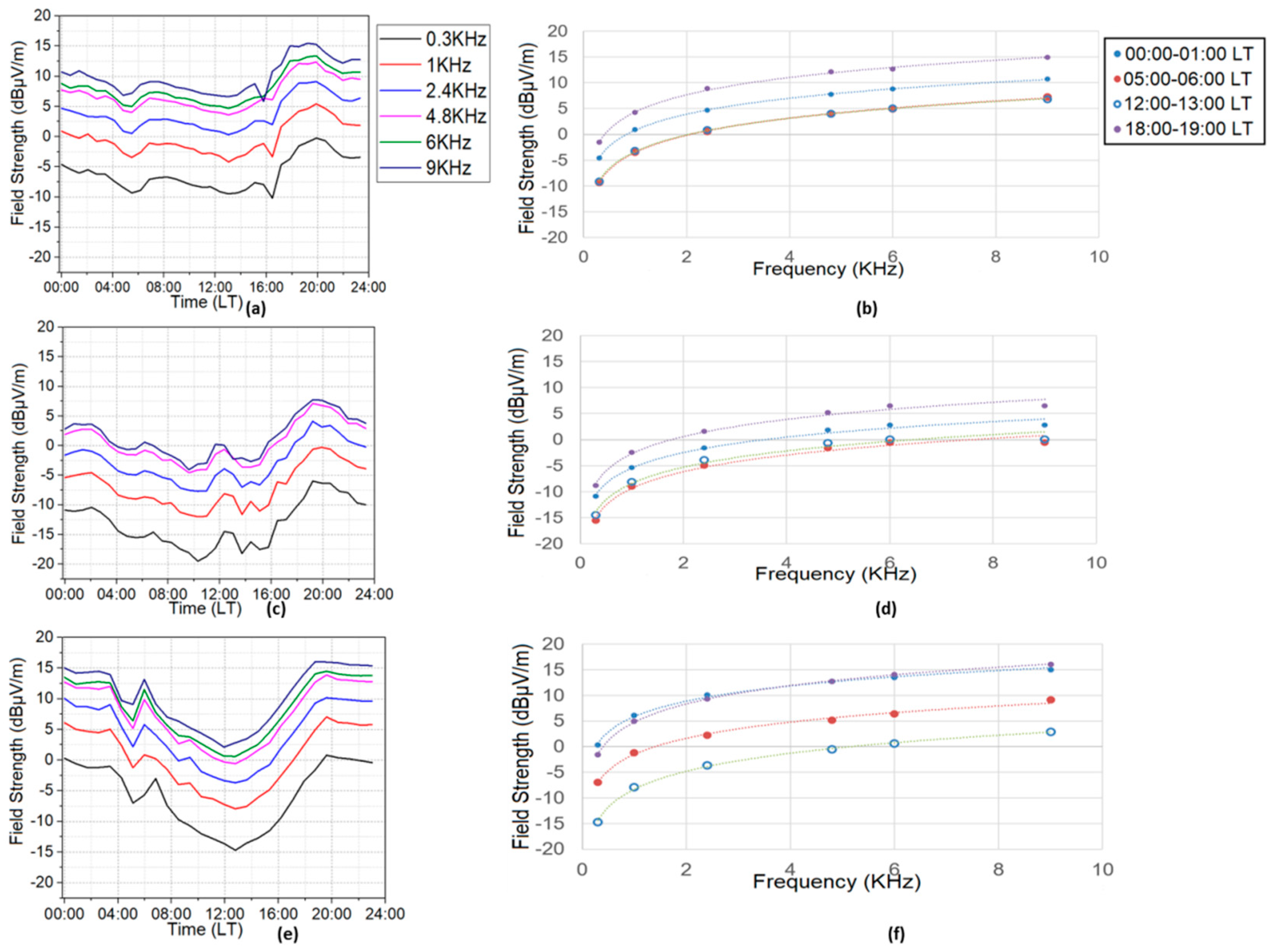
The HF noise diurnal profiles, as a result of scans from consecutive measurements using different bandwidths within an hour, as shown in Figure 8, is demonstrated in Figure 9a,c,e. Figure 7 diurnal curves are based on 144 scans each (as they were spread on six different days). Despite the fact that Figure 9 curves are based on 35 points for allocations 34, and 42 and 28 points for allocation 28 (which is wider), we still had enough scans to derive the diurnal profile for every bandwidth. Based on Figure 9a,c,e, we can deduce the remarkable similarity of the diurnal profile at every bandwidth considered, which supports the hypothesis that the temporal differences in Figure 7 are not based on the different bandwidths used, but rather on the fact that the temporal correlation breaks due to day-to-day differences in HF measurements.
Figure 9b,d,f show HF noise measurements against different bandwidth values within an hour, and an effort to fit this variation with logarithmic functions, which achieve a remarkable approximation to measured values. The logarithmic function used for fitting the variations with the coefficients are given below (Table 2).
We can therefore conclude that within a particular hour, it is clear that a non-linear function is appropriate to describe the variation of HF noise with bandwidth. For a filter bandwidth variation of HF noise to be included in a candidate HF noise model, the independence of bandwidth variation of HF noise with time is therefore established. Since such an independence is established, the reduction of measurement bandwidths within a future campaign will not matter, since HF noise can be successfully predicted for other bandwidths under a logarithmic specification.
4. Conclusions
In this study, using a dataset of just over a month of electric field strength measurements recorded in Cyprus, we have attempted to reveal the main features of HF noise with respect to its temporal, bandwidth, and azimuthal variation. We conclude that there are clear systematic features that provide sufficient evidence for a possible HF noise model specification over the eastern Mediterranean using a more extended dataset in the near future. Such a regional HF noise specification would be useful in order to select an appropriate relay station for a particular time during the day based on its azimuth and the expected noise levels in that particular direction at a particular communication bandwidth. In the future, we plan to extend our investigation by redesigning our HF noise measurement campaign so that we will be able to assemble a much more extensive dataset that would facilitate the study of the statistical distribution of HF noise and how this varies in accordance to season.
Author Contributions
Conceptualization, H.H.; methodology, H.H.; formal analysis, A.C., H.H. and K.S.P.; investigation, A.C. and H.H.; data curation, A.C. and H.H.; writing—original draft preparation, H.H.; writing—review and editing, A.C. and H.H.; visualization, K.S.P.; supervision, H.H.; project administration, A.C.; funding acquisition, A.C. and H.H. All authors have read and agreed to the published version of the manuscript.
Funding
This research was funded by the project “Extending HF Interference Studies over Cyprus” (EHISOC)-POST-DOC/0718/0149, which is co-funded by the Republic of Cyprus and the European Regional Development Fund (through the DIDAKTOR ‘POST DOCTORAL RESEARCHERS’ RESTART 2016–2020 Programme for Research, Technological Development and Innovation).
Data Availability Statement
Not applicable.
Conflicts of Interest
The authors declare no conflict of interest.
References
- Hagn, G.; Stehle, R.; Harnish, L. Shortwave broadcasting band spectrum occupancy and signal levels in the continental United States and Western Europe. IEEE Trans. Broadcast. 1988, 34, 115–125. [Google Scholar] [CrossRef]
- Economou, L.; Haralambous, H.; Green, P.; Gott, G.; Laycock, P.; Broms, M.; Boberg, S. Aspects of HF spectral occupancy. In Proceedings of the Eighth International Conference on HF Radio Systems and Techniques, Venue University of Surrey, Guildford, UK, 10–13 July 2000. [Google Scholar]
- Pederick, L.H.; Cervera, M.A. Modeling the interference environment in the HF band. Radio Sci. 2016, 51, 82–90. [Google Scholar] [CrossRef] [Green Version]
- Economou, L.; Haralambous, H.; Pantjairos, C.; Green, P.; Gott, G.; Laycock, P.; Bröms, M.; Boberg, S. Models of HF spectral occupancy over a sunspot cycle. IEE Proc. Commun. 2005, 152, 980–988. [Google Scholar] [CrossRef]
- Mostafa, G.; Tsolaki, E.; Haralambous, H. HF Spectral Occupancy Time Series Models Over the Eastern Mediterranean Region. IEEE Trans. Electromagn. Compat. 2016, 59, 240–248. [Google Scholar] [CrossRef]
- Haralambous, H.; Papadopoulos, H. 24-Hour Neural Network Congestion Models for High-Frequency Broadcast Users. IEEE Trans. Broadcast. 2009, 55, 145–154. [Google Scholar] [CrossRef]
- Haralambous, H.; Papadopoulos, H. 24-h HF Spectral Occupancy Characteristics and Neural Network Modeling over Northern Europe. IEEE Trans. Electromagn. Compat. 2017, 59, 1817–1825. [Google Scholar] [CrossRef]
- Cecil, D.J.; Buechler, D.E.; Blakeslee, R.J. Gridded lightning climatology from TRMM-LIS and OTD: Dataset description. Atmos. Res. 2014, 135–136, 404–414. [Google Scholar] [CrossRef] [Green Version]
- Coleman, C.J. A direction-sensitive model of atmospheric noise and its application to the analysis of HF receiving antennas. Radio Sci. 2002, 37, 3-1–3-10. [Google Scholar] [CrossRef] [Green Version]
- Kotaki, M. Global distribution of atmospheric radio noise derived from thunderstorm activity. J. Atmos. Terr. Phys. 1984, 46, 867–877. [Google Scholar] [CrossRef]
- Watterson, C.C.; Juroshek, J.R.; Bensema, W.D. Experimental confirmation of an HF channel model. IEEE Trans. Commun. Technol. 1970, 18, 792–803. [Google Scholar] [CrossRef]
- Ibukun, O. Measurements of atmospheric noise levels. Radio Electron. Eng. 1964, 28, 405–415. [Google Scholar] [CrossRef]
- Ibukun, O. Structural aspects of atmospheric radio noise in the tropics. Proc. IEEE 1966, 54, 361–367. [Google Scholar] [CrossRef]
- Giesbrecht, J.; Clarke, R.; Abbott, D. An empirical study of the probability density function of HF noise. Fluct. Noise Lett. 2006, 6, L117–L125. [Google Scholar] [CrossRef] [Green Version]
- Lemmon, J.J.; Behm, C.J. Wideband HF Noise/Interference Modeling Part I: First-Order Statistics; Technical Report 91-277; U.S. Department of Commerce, National Telecommunications and Information Administration (NTIA): Washington, DC, USA, 1991.
- Lemmon, J.J.; Behm, C.J. Wideband HF Noise/Interference Modeling Part II: Higher-Order Statistics; Technical Report 93-293; U.S. Department of Commerce, National Telecommunications and Information Administration (NTIA): Washington, DC, USA, 1993.
- Lemmon, J.J. Wideband model of HF atmospheric radio noise. Radio Sci. 2001, 36, 1385–1391. [Google Scholar] [CrossRef]
- Ward, B.; Golley, M. Solar cycle variations in atmospheric noise at HF. In Proceedings of the Fifth International Conference on HF Radio Systems and Techniques, Edinburgh, UK, 22–25 July 1991; IET: Edinburgh, UK, 1991; pp. 327–331. [Google Scholar]
- Rodriguez, S.P. High-frequency noise and spectrum occupancy measurements for Virginia and Texas with comparisons to International Radio Consultative Committee predictions. Radio Sci. 1997, 32, 2075–2082. [Google Scholar] [CrossRef]
- Shinde, M.; Gupta, S. A Model of HF Impulsive Atmospheric Noise. IEEE Trans. Electromagn. Compat. 1974, EMC-16, 71–75. [Google Scholar] [CrossRef]
- Pederick, L.H.; Cervera, M.A. A directional HF noise model: Calibration and validation in the Australian region. Radio Sci. 2016, 51, 25–39. [Google Scholar] [CrossRef] [Green Version]
- Georgiou, G. British bases in Cyprus and signals intelligence. Études Helléniques/Hell. Stud. 2011, 19, 121–130. [Google Scholar]
- Posa, L.M.; Materazzi, D.J.; Gerson, N.C. Azimuthal variation of measured HF noise. IEEE Trans. Electromagn. Compat. 1972, 1, 21–31. [Google Scholar] [CrossRef]
- Gibson, A.J.; Arnet, L. Azimuthal Distribution of Noise and Interference at HF. In Proceedings of the 8th International Conference in Antennas & Propagation, Edinburgh, UK, 30 March–2 April 1993. Publication No. 370. [Google Scholar]
- International Radio Consultative Committee (CCIR). Characteristics and Applications of Atmospheric Radio Noise Data; Technical Report 322-3; International Telecommunication Union: Geneva, Switzerland, 1986. [Google Scholar]
- Wong, N.; Gott, G.; Barclay, L. HF spectral occupancy and frequency planning. IEE Proc. F Commun. Radar Signal Process. 1985, 132, 548–557. [Google Scholar] [CrossRef]
- Gott, G.F.; Chan, S.K.; Pantjiaros, C.A.; Brown, J.; Laycock, P.; Broms, M.; Boberg, S. Recent work on the measurement and analysis of spectral occupancy at HF. In Proceedings of the Sixth International Conference on HF Radio Systems and Techniques, Venue University of, York, York, UK, 4–7 July 1994. [Google Scholar]
- Andersson, A. Bandwidth and range dependence of HF interference statistics. In Proceedings of the Fifth International Conference on HF Radio Systems and Techniques, Edinburgh, UK, 22–25 July 1991. [Google Scholar]
- Array Solutions Website. Available online: https://www.arraysolutions.com/ (accessed on 30 October 2022).
Figure 1.
(a) Measurement system, (b) SAL-12 antenna.

Figure 2.
Electric field strength measurement scans with the SAL-12 antenna steered north-west for 8.500–8.815 MHz in the interval (a) 13:20–13:30 LT and (b) 23:50–00:00 LT.
Figure 2.
Electric field strength measurement scans with the SAL-12 antenna steered north-west for 8.500–8.815 MHz in the interval (a) 13:20–13:30 LT and (b) 23:50–00:00 LT.

Figure 3.
Diurnal profiles of HF noise on consecutive HF allocations from 12 June to 5 July 2022.

Figure 4.
Diurnal variation of HF noise as a function of frequency.

Figure 5.
Diurnal profile of azimuthal RMS noise field strength measurements on (a) 13 June 2022 for 7.3–7.8 MHz and (b) 4 July 2022 for 25.67–26.1 MHz.
Figure 5.
Diurnal profile of azimuthal RMS noise field strength measurements on (a) 13 June 2022 for 7.3–7.8 MHz and (b) 4 July 2022 for 25.67–26.1 MHz.
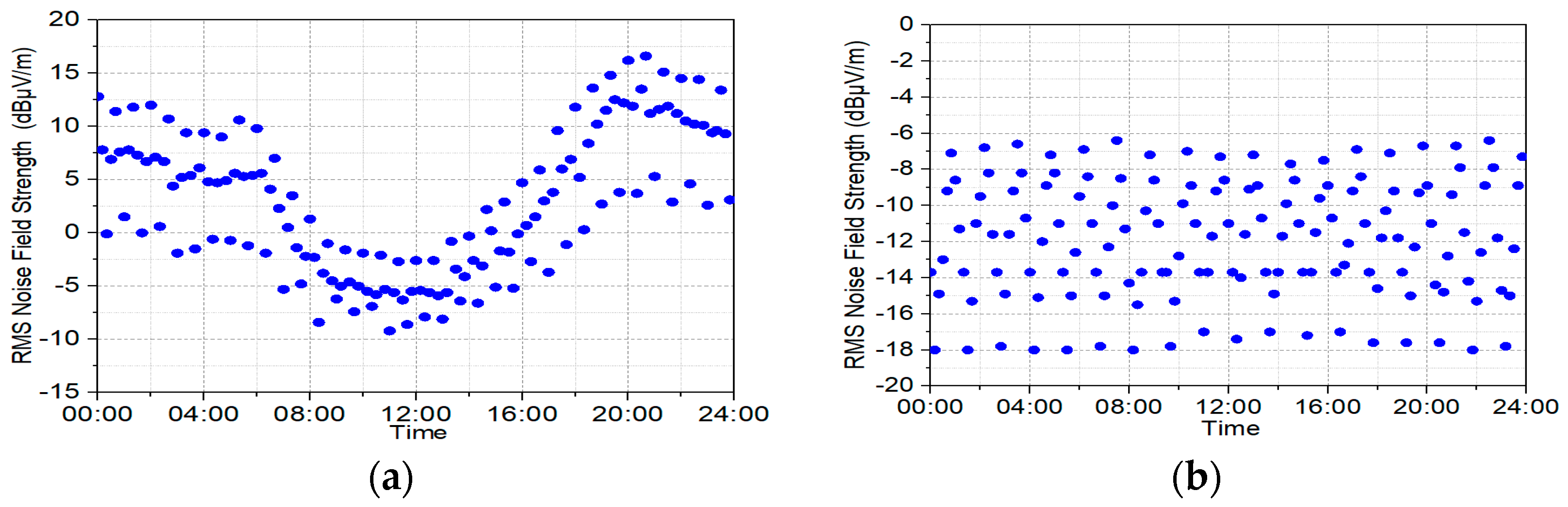
Figure 6.
Azimuthal HF noise profile for 00:00–05:00 (a) at 7.3–7.8 MHz and (b) 16.86–17.41 MHz.
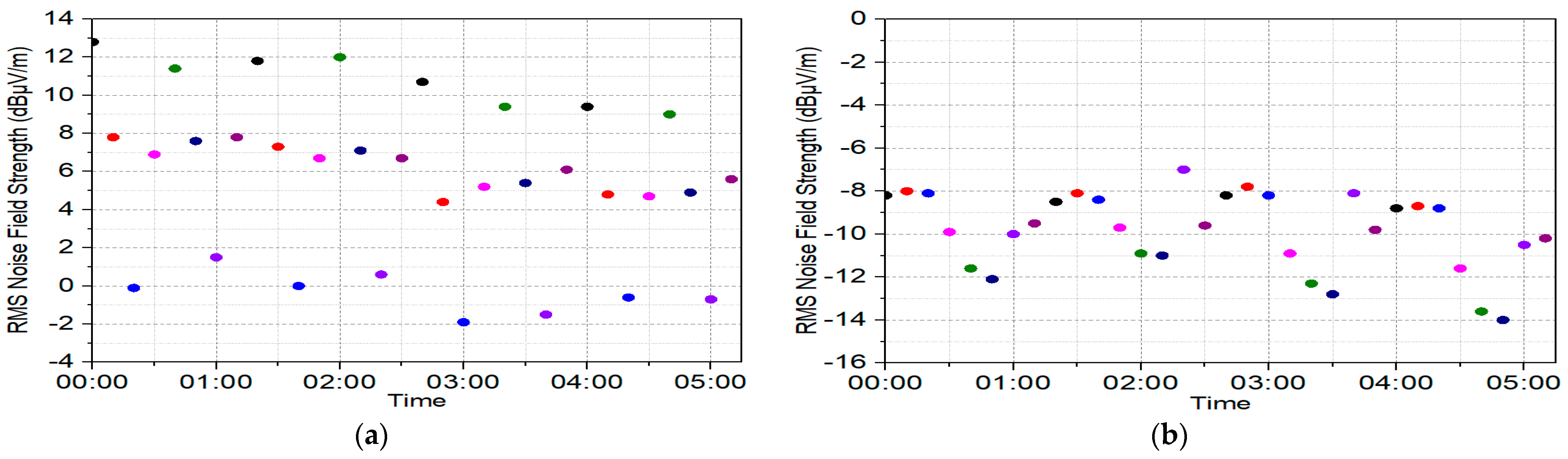
Figure 7.
Diurnal profiles at 10-min resolution of HF noise field strength measurements for various filter BWs at different consecutive days for 9.50–9.90 MHz.
Figure 7.
Diurnal profiles at 10-min resolution of HF noise field strength measurements for various filter BWs at different consecutive days for 9.50–9.90 MHz.
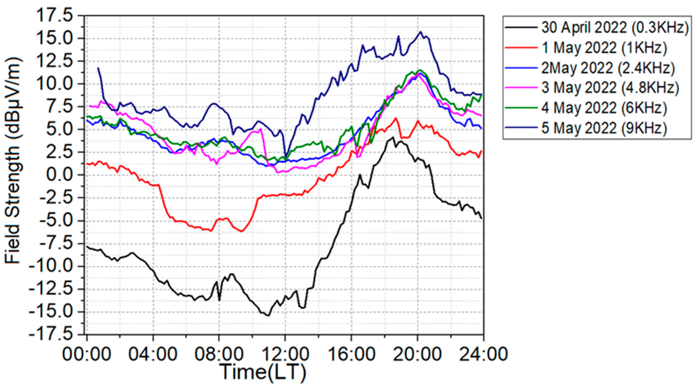
Figure 8.
Scans with the SAL-12 antenna steered north for 9.5–9.9 MHz during 15:00–16:00 LT with a filter bandwidth of (a) 0.3 kHz, (b) 1.0 kHz, (c) 2.4 kHz, (d) 4.8 kHz, (e) 6.0 kHz, and (f) 9.0 kHz.
Figure 8.
Scans with the SAL-12 antenna steered north for 9.5–9.9 MHz during 15:00–16:00 LT with a filter bandwidth of (a) 0.3 kHz, (b) 1.0 kHz, (c) 2.4 kHz, (d) 4.8 kHz, (e) 6.0 kHz, and (f) 9.0 kHz.
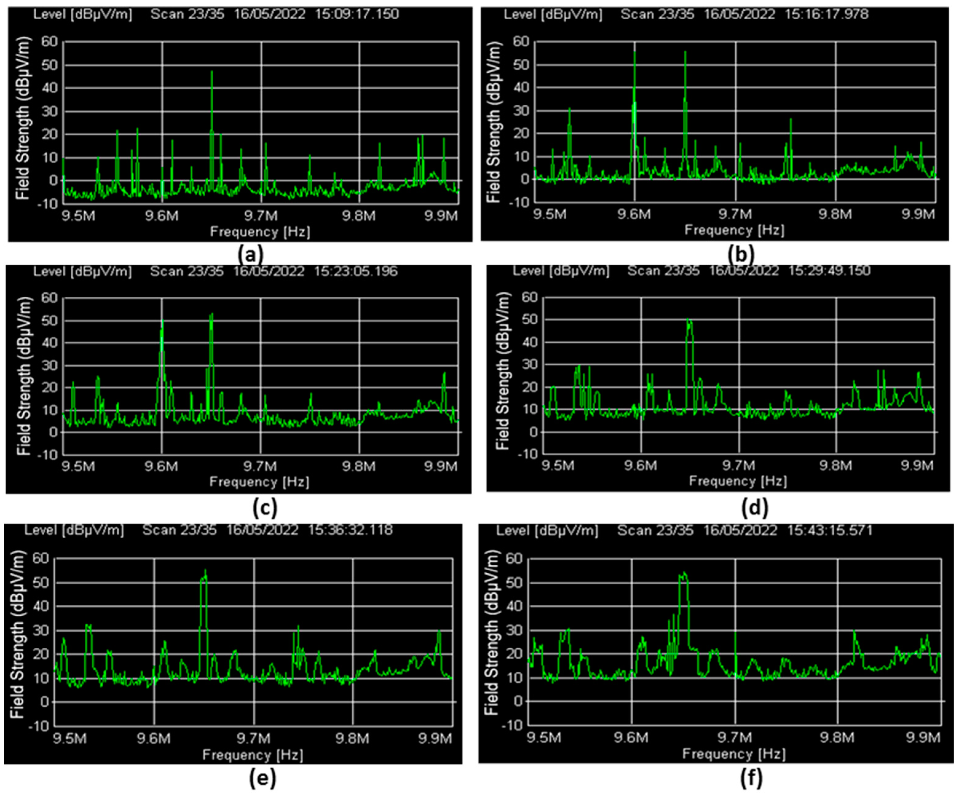
Figure 9.
Diurnal profile of HF noise (left) and HF noise field strength measurements as a function of filter BW with logarithmic fitted functions (right) for (a,b) 7.3–7.8 MHz on 16 May, for (c,d) 9.5–9.9 MHz on 17 May and (e,f) 11.65–12.05 MHz on 18 May.
Figure 9.
Diurnal profile of HF noise (left) and HF noise field strength measurements as a function of filter BW with logarithmic fitted functions (right) for (a,b) 7.3–7.8 MHz on 16 May, for (c,d) 9.5–9.9 MHz on 17 May and (e,f) 11.65–12.05 MHz on 18 May.

Table 1.
ITU HF Frequency Allocations.
| Code | Primary Users | Frequency (MHz) | Code | Primary Users | Frequency (MHz) |
|---|---|---|---|---|---|
| 1 | FIXED/MOBILE | 1.606–1.810 | 49 | FIXED/MOBILE | 13.800–14.000 |
| 2 | AMATEUR | 1.810–1.850 | 50 | AMATEUR | 14.000–14.350 |
| 3 | FIXED/MOBILE | 1.850–2.045 | 51 | FIXED/MOBILE | 14.350–15.000 |
| 4 | FIXED/MOBILE | 2.045–2.300 | 52 | AEROMOBILE | 15.000–15.100 |
| 5 | FXD./MOB./BCST. | 2.300–2.500 | 53 | BROADCAST | 15.100–15.600 |
| 6 | FIXED/MOBILE | 2.500–2.850 | 54 | FIXED | 15.600–16.000 |
| 7 | AEROMOBILE | 2.850–3.155 | 55 | FIXED | 16.000–16.360 |
| 8 | FIXED/MOBILE | 3.155–3.200 | 56 | MARITIME/MOB. | 16.360–16.860 |
| 9 | FXD./MOB./BCST. | 3.200–3.400 | 57 | MARITIME/MOB. | 16.860–17.410 |
| 10 | AEROMOBILE | 3.400–3.500 | 58 | FIXED | 17.410–17.550 |
| 11 | FXD./MOB./AMTR. | 3.500–3.800 | 59 | BROADCAST | 17.550–17.900 |
| 12 | FIXED/MOBILE | 3.800–3.900 | 60 | AEROMOBILE | 17.900–18.030 |
| 13 | AEROMOBILE | 3.900–3.950 | 61 | FIXED | 18.030–18.068 |
| 14 | FIXED/BCST. | 3.950–4.000 | 62 | AMATEUR | 18.068–18.168 |
| 15 | MARITIME/MOB. | 4.000–4.438 | 63 | FIXED/MOBILE | 18.168–18.780 |
| 16 | FIXED/MOBILE | 4.438–4.650 | 64 | MARITIME/MOB | 18.780–18.900 |
| 17 | AEROMOBILE | 4.650–4.750 | 65 | FIXED | 18.900–19.300 |
| 18 | FXD./MOB./BCST. | 4.750–5.060 | 66 | FIXED | 19.300–19.680 |
| 19 | FIXED/MOBILE | 5.060–5.480 | 67 | MAR/MOB | 19.680–19.800 |
| 20 | AEROMOBILE | 5.480–5.730 | 68 | FIXED | 19.800–20.000 |
| 21 | FIXED/MOBILE | 5.730–5.950 | 69 | FIXED/MOBILE | 20.000–20.500 |
| 22 | BROADCAST | 5.950–6.200 | 70 | FIXED/MOBILE | 20.500–21.000 |
| 23 | MARITIME/MOB. | 6.200–6.525 | 71 | AMATEUR | 21.000–21.450 |
| 24 | AEROMOBILE | 6.525–6.765 | 72 | BROADCAST | 21.450–21.870 |
| 25 | FIXED/MOBILE | 6.765–7.000 | 73 | AEROMOBILE | 21.870–22.000 |
| 26 | AMATEUR | 7.000–7.100 | 74 | MAR/MOB | 22.000–22.400 |
| 27 | BROADCAST | 7.100–7.300 | 75 | MAR/MOB | 22.400–22.855 |
| 28 | FIXED/MOBILE | 7.300–7.800 | 76 | FIXED | 22.855–23.000 |
| 29 | FIXED/MOBILE | 7.800–8.195 | 77 | FIXED/MOBILE | 23.000–23.200 |
| 30 | MARITIME/MOB. | 8.195–8.500 | 78 | AEROMOBILE | 23.200–23.350 |
| 31 | MARITIME/MOB. | 8.500–8.815 | 79 | FIXED/MOBILE | 23.350–24.000 |
| 32 | AEROMOBILE | 8.815–9.040 | 80 | FIXED/MOBILE | 24.000–24.500 |
| 33 | FIXED | 9.040–9.500 | 81 | FIXED/MOBILE | 24.500–24.890 |
| 34 | BROADCAST | 9.500–9.900 | 82 | AMATEUR | 24.890–25.000 |
| 35 | FIXED | 9.900–10.000 | 83 | MAR/MOB | 25.000–25.210 |
| 36 | AEROMOBILE | 10.000–10.100 | 84 | FIXED/MOBILE | 25.210–25.550 |
| 37 | FIXED/AMATEUR | 10.100–10.150 | 85 | RAD/ASTR | 25.550–25.670 |
| 38 | FIXED/MOBILE | 10.150–10.600 | 86 | BROADCAST | 25.670–26.100 |
| 39 | FIXED/MOBILE | 10.600–11.175 | 87 | MAR/MOB | 26.100–26.175 |
| 40 | AEROMOBILE | 11.175–11.400 | 88 | FIXED/MOBILE | 26.175–26.500 |
| 41 | FIXED | 11.400–11.650 | 89 | FIXED/MOBILE | 26.500–27.000 |
| 42 | BROADCAST | 11.650–12.050 | 90 | FIXED/MOBILE | 27.000–27.500 |
| 43 | FIXED | 12.050–12.230 | 91 | FXD./MOB./METR. | 27.500–28.000 |
| 44 | MARITIME/MOB. | 12.230–12.730 | 92 | AMATEUR | 28.000–28.500 |
| 45 | MARITIME/MOB. | 12.730–13.200 | 93 | AMATEUR | 28.500–29.000 |
| 46 | AEROMOBILE | 13.200–13.360 | 94 | AMATEUR | 29.000–29.700 |
| 47 | FIXED/MOBILE | 13.360–13.600 | 95 | FIXED/MOBILE | 29.700–30.000 |
| 48 | BROADCAST | 13.600–13.800 |
Table 2.
List of coefficients used for fitting the variations noted in the hourly bandwidth.
| Date | Time (LT) | Coefficients | ||
|---|---|---|---|---|
| a | b | R2 (Regression Coefficient) | ||
| 16 May | 00:00–01:00 | 4.4681 | 0.811 | 0.9998 |
| 05:00–06:00 | 4.8137 | 3.5286 | 0.9997 | |
| 12:00–13:00 | 4.6687 | 3.3405 | 0.9996 | |
| 18:00–19:00 | 4.8339 | 4.3205 | 0.9986 | |
| 17 May | 00:00–01:00 | 4.2812 | 5.4494 | 0.9859 |
| 05:00–06:00 | 4.6309 | 9.3809 | 0.9831 | |
| 12:00–13:00 | 4.5166 | 8.4263 | 0.9793 | |
| 18:00–19:00 | 4.756 | 2.7083 | 0.9866 | |
| 18 May | 00:00–01:00 | 4.3306 | 5.8475 | 0.9968 |
| 05:00–06:00 | 4.5531 | 1.5364 | 0.9954 | |
| 12:00–13:00 | 5.0691 | 8.3228 | 0.9985 | |
| 18:00–19:00 | 5.165 | 4.7453 | 0.9996 | |
Publisher’s Note: MDPI stays neutral with regard to jurisdictional claims in published maps and institutional affiliations. |
© 2022 by the authors. Licensee MDPI, Basel, Switzerland. This article is an open access article distributed under the terms and conditions of the Creative Commons Attribution (CC BY) license (https://creativecommons.org/licenses/by/4.0/).
Share and Cite
MDPI and ACS Style
Haralambous, H.; Constantinides, A.; Paul, K.S. HF Noise Characteristics over Cyprus. Remote Sens. 2022, 14, 6040. https://doi.org/10.3390/rs14236040
AMA Style
Haralambous H, Constantinides A, Paul KS. HF Noise Characteristics over Cyprus. Remote Sensing. 2022; 14(23):6040. https://doi.org/10.3390/rs14236040
Chicago/Turabian StyleHaralambous, Haris, Antonios Constantinides, and Krishnendu Sekhar Paul. 2022. "HF Noise Characteristics over Cyprus" Remote Sensing 14, no. 23: 6040. https://doi.org/10.3390/rs14236040
Note that from the first issue of 2016, this journal uses article numbers instead of page numbers. See further details here.