Article

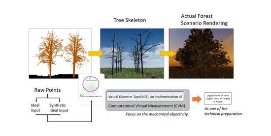
Integrating Real Tree Skeleton Reconstruction Based on Partial Computational Virtual Measurement (CVM) with Actual Forest Scenario Rendering: A Solid Step Forward for the Realization of the Digital Twins of Trees and Forests

1
National Danzhou Investigation and Experiment Station of Tropical Crops, Rubber Research Institute, Chinese Academy of Tropical Agricultural Sciences, Danzhou 571737, China
2
College of Information Science and Technology, Nanjing Forestry University, Nanjing 210037, China
3
Beijing Key Laboratory of Precision Forestry, Beijing Forestry University, Beijing 100083, China
4
Department of Earth Observation, Friedrich-Schiller-University Jena, 07743 Jena, Germany
5
Department of Geography, Friedrich-Schiller-University Jena, 07743 Jena, Germany
6
Research Institute of Forestry Resource Information Techniques, Chinese Academy of Forestry, Beijing 100091, China
*
Author to whom correspondence should be addressed.
These authors contributed equally to this work.
Remote Sens. 2022, 14(23), 6041; https://doi.org/10.3390/rs14236041
Submission received: 30 August 2022 / Revised: 19 November 2022 / Accepted: 21 November 2022 / Published: 29 November 2022
(This article belongs to the Special Issue Remote Sensing and Smart Forestry)

Abstract

:
Digital twins of forests (trees) are computational virtual recreations of forests (trees) in which the entity distributions and physical processes in real-world forests (trees) are duplicated. It is expected that conventional forest science and management can be undertaken in a digital twin of forests (trees) if the recreation of a real-world forest (tree) has accurate and comprehensive enough information. However, due to the various differences between the current tree model and the real tree, these envisioned digital twins of the forests (trees) stay a theoretical concept. In this study, we developed a processing strategy that partially integrated computational virtual measurement (CVM) process into the tree modeling workflow. Owing to the feature of CVM, partial tree skeleton reconstruction procedures were considered to have higher mechanical objectivity compared to conventional mathematical modeling methods. The reason was that we developed a novel method called virtual diameter tape (VDT), which could provide a certain percentage of modeling elements using CVM. Technically, VDT was able to virtually measure diameters and spatial distribution of cross-sectional area of trees, including the basal area, from point clouds. VDT simulated the physical scenario of diameter tapes, observing point clouds of trees. Diameter and the cross-sectional area of stem and branches were obtained by two consecutive physical measurement processes, one in the forest sample site and another in the virtual space. At the same time, VDT obtained better or a similar accuracy compared to the mathematical methods, i.e., Hough transform-based methods, using the same data sets. The root-mean-square deviation (RMSE) of retrieval of diameter at breast height (DBH) using VDT was 1.02 cm, while DBH obtained from three conventional methods varied from 1.29 cm to 1.73 cm. Based on VDT measurement results, tree skeleton reconstruction and actual forest scenario rendering of our sample plots were further implemented. Beyond the visual consistency, we believe that our work might be a small and solid step in the technological evolution from tree models to the digital twin of forests (trees).

Graphical Abstract

1. Introduction

1.1. Form Tree Models to Digital Twin of Forests

The construction of realistic three-dimensional (3D) tree models is becoming an attractive research focus [1,2,3]. Making a detailed tree model depends on two technological bases. The first and fundamental technology is LiDAR (light detection and ranging) scanning, which records the spatial information of trees at a very high sampling rate [4]. Compared to measures in sample plots using conventional instruments [5], the volume of raw measurement data increases exponentially, which supports tree modeling with high level of detail (LoD) [6]. The second dependency for making a detailed tree model is the computational method. In contrast to the computational virtual measurements (CVM) we employed in this work [7], most of the current methods are mathematically based. For example, quantitative structure models (QSMs) were developed by Raumonen et al. in 2013 [8]. The QSM’s approach considers that a tree can be decomposed into a huge number of little cylinders. A tree model is then generated as a collection of little cylinders. The QSM’s approach utilizes the classical technical route of calculus with great success. Since then, improved QSM methods such as TreeArchitecture [9], Simpleforest [10], and AdQSM [11], have been developed. The implementations of QSMs are booming [12,13,14]. In addition to QSM methods, conventional voxel tree modeling methods are continuously evolving [15]. However, it is more likely to be used as a tool for the estimation of tree and forest parameters [16]. One of the reasons, we think, is that voxel modeling methods are slightly weaker than QSMs in the visual presentation of the model.
Nowadays, increasing studies of the digital twin are reported in a variety of different fields [17,18]. However, the concept and clear definition of the digital twin of trees and the digital twin of forests are rarely discussed [19]. From our point of view, the deviation between the 3D tree model and the digital twin of the tree is one of the difficulties. What can be expected is that accurate 3D tree models could act as a precursor of digital twin of trees as well as virtual trees. In our previous study, we envisioned that a virtual tree should be an exact digital replica of the corresponding tree in reality [7,20]. However, due to various theoretical and morphological complications, e.g., the topological vagueness of tree structures reflected by remote sensing data, complex internal relevance [21,22,23,24] and the internal logic used in tree modeling [25,26], it seems technically difficult to construct an ideal virtual tree that perfectly maps a real tree, especially in the aspects of bole diameter estimation and tree skeleton reconstruction [27]. Meanwhile, a clear definition of virtual trees or digital twins of trees has not yet reached a unified consensus in society today. In light of recent trends [28,29,30], the term “realistic” is more likely to refer to visual consistency between real trees and virtual trees [31]. Any further analysis based on visually realistic tree models may raise concerns about objectivity. This is why we cannot regard the existing tree models as equivalent to virtual trees or digital twins of trees.
Equation (1) describes our view of the relationships between digital twins of trees and tree models. A tree model can be considered as a digital twin of tree if every predicational component made by the tree modeling algorithm can be verified. In such a situation, no false competent of trees can be added to the tree model. On this basis, a tree model with higher-level objectivity is constructed, which is an ideal state, i.e., the digital twin of a tree in reality.
d i g i t a l   t w i n   o f   t r e e = lim n 0   t r e e   m o d e l n
where n refers to the amount of unverifiable predictions made by algorithms during tree modeling.
Based on Equation (1), we further assume the technical description of the digital twin of forests. As shown in Equation (2), a digital twin of forest firstly consists of each digital twin of tree and other digital twins, e.g., the digital twin of undergrowth and soil surface. In addition to static expressions, it should also contain the realistic simulation of basic physical and physiological processes of trees and other objects in the forest. In this way, a digital twin of forest, as a toolbox, can support virtual experimentation and produce meaningful data that helps people to understand what could happen in reality.
d i g i t a l   t w i n   o f   f o r e s t = f d i g i t a l   t w i n   o f   t r e e + f o t h e r   d i g i t a l   t w i n
where f x refers to the function of the simulation of basic physical and physiological processes as toolboxes.

1.2. A Step Forward for the Realization of the Digital Twin of Trees

In our previous study, we developed the theory of computational virtual measurement (CVM) and an implementation of CVM, i.e., the virtual water displacement (VWD) method [7]. Compared to conventional mathematical procedures used in processing LiDAR point clouds, CVM simulates physical principles of measuring instruments and measuring procedures to measure point clouds of tree. In terms of algorithmic mechanisms, CVM is superior to mathematical procedures, e.g., tree modeling. This is because the CVM procedure is an observational process and does not make any predictions.
How to improve the mechanical objectivity of the tree modeling process? CVM provides a novel perspective of the utilization of algorithmic logic instead of the need for external reference. In this study, we developed virtual diameter tape (VDT) as a new implementation of CVM. VDT measured the point cloud of trees for the diameter and area of cross-sections of trees. Accordingly, the measurement results provided confident raw references for tree skeleton reconstruction. In addition to the tree skeleton reconstruction, actual forest scenario rendering was further implemented. Thus, compared to tree modeling using pure mathematical processes, this integrated workflow earned a small step toward better mechanical objectivity.
The mechanical objectivity of VDT depends on the precise duplication of the physical scenario of the diameter tape. The diameter tape was developed in earlier times and is still in use nowadays [32]. Explicit and simple physical processes are employed by these measuring instruments, while predictive mathematical processes are excluded. For example, a diameter tape makes physical contact with a tree stem in the position of the diameter at breast height (DBH) [33]. The measurement process is subdivided by us into several steps, and all of them are physical processes. In the beginning, the diameter tape encloses an arbitrary-shaped area, including the stem inside. Then, the diameter tape starts to shrink in space. In this process, the shape of the enclosed area gradually approaches the measurement object. In other words, areas that do not belong to the cross-sectional area are gradually excluded by the movement of the diameter tape. Theoretically, when all the redundant areas are excluded, we can obtain an exactly true DBH. In the final step, the termination signal of the measurement completion is also physical. First, diameter tape has no chance to cross the inner part of the stem. Second, the diameter tape is in contact with each point on the surface of the stem and cannot be further constricted by external forces from human operators. Despite the fact that human influence on physical processes has led to the need for non-predictive mathematical processes, such as the calculation of the mean value [33,34], we believe that the high objectivity of measurement using diameter tape is granted by its own processes. The key is that measurements using diameter tapes are purely physical processes, with no need for any mathematical preset of the measured objects.
As a widely used data source for tree modeling, LiDAR scanners use completely different physical mechanisms from that used by diameter tape to collect tree information. The sensor in LiDAR scanners records the distance between the sensor and the laser-irradiated spot [35]. Compared to diameter tapes, the beam emitted by the sensor travels in a straight line and cannot encircle the stem. Accordingly, the spatial information of the outline of the stem is unable to be determined in the raw measurement data of a single beam. We believe that this is the first decline in objectivity. As compensation for the loss of physical mechanism, the LiDAR sensor projects dense beams on the measuring target [36]. It uses rotating mirrors to deflect the beam to cover the necessary stem area [37]. The motion of the rotating mirror is controlled by a gear drive mechanism step by step [38]. Each shift of the rotating mirror leads to an independent measuring process. Point clouds are stored as a discrete data set containing the morphologies of each tree component, which are always affected by the instability of apparatus performance and disturbances raised by external environments. Restoring the continuous contours on the bole surface from the discrete data set requires the assistance of computer algorithms [39] and additional mathematical derivation [40]. Conversely, employing a diameter tape [41] causes a cumbersome experimental measurement process, especially for branches at the higher parts of forest canopy [42]. Moreover, manual measurement always reduces overall mechanical objectivity and results in unavoidable artificial errors.
The primary problem of the mathematical procedure is that there is a deviation between the shape of the natural stem and the human-defined stem using mathematical approaches. For example, commonly used approaches based on the concepts of circle fitting the approximate contour of the basal area of the stem [43,44], such as the Monte Carlo method [45], Hough transformation [46], random sample consensus (RANSAC) [47], and 3D modeling [48], are always restricted by the pre-definition of the regular shape of stem with detrimental factors of original shape restoration. Meanwhile, due to the lack of objectivity at the mechanical level, there is an obligation to provide justifications, which leads to additional workloads [49].
In the evolution from tree models to digital twins of trees, while waiting for the overall evolution of current LiDAR scanning mechanisms and tree modeling methods, we could try different technological routes. With this work, we employed CVM as an efficient tool for measuring the diameter of the bole and branches. Meanwhile, the phenotypic traits of the tree skeleton can be graphically portrayed in pursuit of forest plot scenario reconstruction with high fidelity and enhanced immersion in a parallel spatiotemporal continuum. Meanwhile, trees in different growth stages and development situations were recorded in detail and realistically visualized, which affords historic characterizations and comprehensive information to guide current forest cultivation practices and silvicultural managements.

2. Material and Methods

2.1. Study Area and Field Measurements

The study area was located in the Hainan Province, China, between (109°43′E, 19°28′N) and (109°51′E, 19°38′N) with an area of 5000 ha. The main landform type is hilly plateau, and the average altitude is 188 m. The climate type is tropical savanna climate. Since the 1950s, rubber trees (Hevea brasiliensis) have been planted extensively for commercial purposes in this area. Presently, rubber plantations cover ca. 3000 ha. Due to the complicated ownership of property, rubber trees of each age group are mixed together and have not developed a clear spatial pattern if we observe from the sky.
Three sample plots of rubber trees were measured as shown in Figure 1d. The average tree ages in those sample plots were five years, ten years, and twenty years old, respectively. As shown in Figure 1a, each sample plot consisted of ten trees surrounded by five LiDAR scan positions. All rubber trees in sample plots were planted in a narrow-wide-row planting pattern (2 m by 4 m). We used Leica ScanStation C10 for scanning. The primary capabilities of Leica ScanStation C10 were listed as the following: accuracy of single measurement, 6 mm (position), 4 mm (distance); target acquisition, 2 mm std. deviation; range, 300 m at 90%; 134 m at 18% albedo (minimum range 0.1 m); scan rate, up to 50,000 points/sec, maximum instantaneous rate. Figure 1b shows the obtained point clouds from the five-year-old rubber tree sample plot. Figure 1c shows a photo of when a LiDAR scan was performed.
In addition to LiDAR scanning, conventional field measurements, collecting three tree variables, were performed. These measurements provided a ground truth reference for evaluating new methods developed in this study. First of all, diameter of breast height (DBH) was measured using plastic diameter tape for each tree. Then, the stem diameter at an arbitrary height along a tree bole was measured using diameter tape or a novel diameter clipper [50].
The third variable was the diameter of first-order branches. This work was labor-intensive and could not be applied to each tree in the three sample plots. Therefore, three adjacent trees in each sample plot were picked and then measured. The criterion for the selection of the sample trees was point cloud completeness. Therefore, these measurements were performed after the data preprocessing. We inspected the aligned point clouds of each sample plot to find trees with relatively minor defects. Then, crews in our survey team built and climbed scaffoldings and performed measurements of the branch base diameters for three trees in each sample plot.

2.2. Data Preprocessing

Point clouds of ten trees from each sample plot, for a total of 30 trees, were used to carry out VDT measurement and create forest scenario rendering. To prepare the qualified inputs, we first performed a data preprocessing work. As shown in Figure 2, this work consisted of two sections. The first section was the conventional data preprocessing procedure for the ground LiDAR scanning. The second section was the amelioration procedure for the new method developed in this study.

2.2.1. Conventional Data Preprocessing

The technical steps in data preprocessing included registration of point clouds from scanning stations, normalization of point cloud height, single tree segmentation, wood-leaf segmentation, and making slices of tree components. Depending on conditions, each slice could be identified as an ideal point cloud [7,51], or a non-ideal point cloud. For the non-ideal point clouds, a mathematical procedure was further applied (in Section 2.2.2). After that, all point clouds were regarded as ideal point clouds.
For registration, Cyclone (Leica Geosystem, Switzerland) software was used to align multi-station point cloud data. The root-mean-square error (RMSE) varied from 4.1 mm to 8.9 mm. In addition to registration, we applied manual deletion of abnormal objects in the aligned point cloud, such as people being scanned and rubber collectors attached to trees. After that, the denoising process was applied using various commonly used filters [3,52] to eliminate the isolated points with the aim of reserving compact tree point clouds. We used a progressive morphological filter to classify ground and non-ground points [53], and the ground points were removed. Consequently, we applied the previously developed individual tree segmentation method to separate point clouds to individual trees [2], and a wood-leaf segmentation algorithm was adopted here for bole and branch component extraction [52]. This single tree point cloud at the whole tree scale was used to verify the growth direction of the stem, and provided the projection coefficient for the following step [54]. A cross-section of the tree skeleton was sliced for stem diameter assessment. Slicing was performed every 0.5 m along the stems. There were thirty trees in total, ten trees in each age group with the acquired horizontal slices obtained. These prepared inputs for the VDT method could be regarded as the tree skeleton presented in the form of point clouds. From an informatics perspective, points are disordered data. The rest of the process of this work was designed to establish order out of disorder.

2.2.2. Amelioration of the Quality of the Wood Points with Gap Filling

A significant proportion of the raw data was made up of non-ideal point clouds, which caused errors in VDT measurement. The function of the amelioration was to make synthetic ideal point clouds that serve as qualifying inputs for VDT. The ideal point cloud is a concept we developed in our previous work [7]. It refers to a point cloud with a high point cloud density, and the gap between each point is generally even. If this condition is not satisfied, then a point cloud is a non-ideal point cloud.
The ideal situation of the collected point clouds should uniformly cover the entire surface of the tree’s woody facets. However, in the interlocked forest plot, mutual occlusion effects by vegetative elements make an occlusion-free position impossible to arrange, as the terrestrial laser scanners for acquainting the data for all the details of the tree body is impracticable, resulting in many tree branches and twigs not being fully hit by laser beams and the gaps emerging in the extracted slice contours regarding local point cloud deficiency. Hence, filling the gaps based on ellipse-fitting methods was deployed herein.
Figure 3 shows the workflow of the amelioration process. When the LiDAR scan failed to capture an ideal point cloud of a cross-section of stem (in Figure 3a), a non-ideal point cloud would be generated. In Figure 3b, we used purple points to represent the recorded points and white points to represent the missed points. To prevent the VDT detector from moving within the internal area in the woods, the missing area (white points) had to be compensated for. In Figure 3c, a fitting circle (red) was employed to enclose the cross-section area. In the next step, a synthetic ideal point cloud was formed through the steps shown in Figure 3d–g. The synthetic ideal point cloud consisted of (purple) points of raw data and (red) synthetic boundary lines. As shown in Figure 3g, a synthetic ideal point cloud preserves the original information from the LiDAR scan, which effectively maintains partial objectivity compared to a pure mathematical fitting as shown in Figure 3c. Finally, a VDT measurement was proceeded on this synthetic ideal point cloud, as shown in Figure 3h. A detailed description of the VDT measurement is Figure 4.
The key process of the amelioration was making the optimal ellipse fitting in Figure 3c, containing three steps: step 1, the determination of the long axis of the fitted ellipse; step 2, the determination of the short axis of the fitted ellipse; and step 3, the determination of the rotation angle of the fitted ellipse. Key mathematical approaches were listed as the following:
Step 1: determination of the long axis of the fitted ellipse.
The input was a cross-section of a tree skeleton. The 3D point cloud was converted to a two-dimensional (2D) point cloud by vertical projection onto the X-Y plane. Then, one or a few incomplete ellipse shapes can be seen in the X-Y plane. P j is used to represent the point set of each individual ellipse, i.e., a slice for each individual trunk or branch. In P j , p i refers to a point in the point cloud set and p i P j . Using the Density-Based Spatial Clustering of Applications with Noise (DBSCAN) algorithm [55], we finally separated the wood point clouds belonging to a fixed height interval into different components P j .
As shown in Figure 4a, an unenclosed ellipse E (in Equation (3)) consisting of point clouds was discernible.
x y 2 a 2 + x sin θ + y cos θ 2 b 2 = 1
where x and y refer to the horizontal and vertical coordinates of the point in the 2D plane, respectively; a and b refer to the lengths of the semi-major and semi-minor axes of the ellipse separately.
The shading effect could be the reason for this. In order to determine the long axis of the fitted ellipse, a straight line l p i p i + 1 containing any two points p i x i , y i and p i + 1 x i + 1 , y i + 1 was randomly selected. There was no order relationship between p i and p i + 1 , which simply represent any two points in P j . The Euclidean distance between p i and p i + 1 was calculated using Equation (4).
p i p i + 1 = x i x i + 1 2 + y i y i + 1 2
where p i and p i + 1 are two randomly selected projection points; x and y refer to the coordinates of the two points.
After iterative selection of any tow points belonging to P j , the maximum value of p i p i + 1 was determined as the potential length of the long axis of the predicted ellipse. It was marked as l p i p i + 1 ( l p i p i + 1 = 2 a in standard pole-polar equation of ellipse). The midpoint of the long axis l p i p i + 1 was marked as p m i d x m i d , y m i d , x m i d = x i + x i + 1 2   y m i d = y i + y i + 1 2 . The slope of l p i p i + 1 was expressed as τ = y i + 1 y i x i + 1 x i . The equation l p i p i + 1 was transformed into Equation (5). Meanwhile, the p m i d x m i d , y m i d was taken as the centroid of the predicted ellipse.
y y i = τ x x i
where x i and y i refer to the coordinates of p i ; x   a n d   y refer to coordinates of the point on the straight line l p i p i + 1 ; τ refers to the slope of l p i p i + 1 .
Step 2: determination of the short axis of the fitted ellipse.
The short axis p k p k + 1 is perpendicular to the long axis l p i p i + 1 of the ellipse and intersected at center point p m i d shown in Figure 4b. Then, the length of short axis was denoted as Equation (6).
p k p k + 1 = x k x k + 1 2 + y k y k + 1 2 = 2 b
where p k and p k + 1 refer to endpoints of the short axis; x   a n d   y refer to coordinates of the endpoints; 2 b refers to the length of short axis of the fitted ellipse.
The predicted short axis could only have one endpoint, i.e., p k + 1 does not exist due to the vacancy of point clouds. In this condition, p k + 1 was used to represent the missing endpoint of the short axis according to the length of p k + 1 p m i d = b and the direction perpendicular to the long axis l p i p i + 1 .
Step 3: determination of the rotation angle of the fitted ellipse.
Before the process of the finding of the optimal value of θ , we performed a coordinate transformation. The coordinate of p c was designed as the coordinate centroid in the 2D Euclidean space. Then, we gradually rotated the ellipse at a pace of π 180 counterclockwise starting from π 2 to π 2 , yielding the translated equation of the fitted ellipse as E r in Equation (7).
E r :   x cos θ y sin θ 2 a 2 + x sin θ + y cos θ 2 b 2 = 1
where x and y refer to the coordinates of the points on the ellipse; a and b refer to the lengths of the semi-major and semi-minor axes of the ellipse, respectively; θ refers to the angle between the long axis of the ellipse and the horizontal axis.
Then, a variable point on the elliptic boundary was defined as q x q , y q , and the distance between p i and q denoted as p i q = x i x q 2 + y i y q 2 . Here, we utilized the Lagrange multiplier method to calculate the minima distance d i m i n between each point p i P j and q , and then the following Lagrange function was constructed as:
F p i , q , μ = f p i , q + μ · φ p i
where p i refers to a random projection point; q refers to a variable point on the elliptic boundary; μ refers to a variable called the “Lagrange multiplier”; φ refers to equation of an ellipse; F x refers to the Lagrange function; f(x) refers to the Euclidean distance between p i and q .
Where f p i , q = x i x q 2 + y i y q 2 and φ p i = x i cos θ y i sin θ 2 a 2 + x i sin θ + y i cos θ 2 b 2 . Solving Equation (8) satisfies the following partial derivative equal to 0 under the conditions of a given value for θ , i.e., F x i = 0 ; F y i = 0 ; F μ = 0 . Then, the distance d i s t s u m between all the projected point sets of any branch slice P j and the fitted rotation ellipse E r at θ angle can be expressed as follows: d i s t s u m = i = 1 N d i m i n , where N represents the total number of points for a branch slice. For all the points of a branch slice, pursuing the rotation angle θ in correspondence to the minimal value of d i s t s u m is the aim of deriving the optimized solution of the rotated ellipse equation, i.e., determination of the rotation angle θ .

2.3. Analysis of Physical Scenario of Diameter Tapes

The successful development of a virtual measurement instrument (VMI) depends on a detailed analysis of the physical scenario of its corresponding real measurement instrument (RMI) [7]. In this study, the principle of the physical mechanism of diameter tape was elucidated, acting as a virtual diameter tape to determine the diameter, perimeter of each branch, and bole in pursuit of the spatial information collection of tree woody facets.
The physical scenario of diameter tapes when measuring DBH is shown in Figure 5a–d. Before the measurement was applied, the space around the stem was physically divided into two regions in Figure 5a. There was a basal area (internal area) and external area. The first encirclement of the stem was achieved by the diameter tape shortly after the start of the measurement process in Figure 5b. Accordingly, an enclosed area was produced by the diameter tape. As shown in Figure 5c, with the continuous shrinking of the diameter tape, the enclosed area was approached the basal area. This process was a non-discrete process. At each moment, the instantaneous closed area could be considered as a measure of the basal area. How to determine the best measure among an infinite number of measures? On the face of it, there was no doubt that the smallest value should be chosen. The objectivity of this choice was supported by the sample and clear termination condition of the measuring process. As shown in Figure 5d, the diameter tape (considered a rigid body) reached a steady state when it had no room for further contraction. This termination condition was independent of the outcome of the measuring process. The exact same physics was utilized each time to measure DBH using the diameter tape. In our opinion, this provides the basis for making the diameter tape a standard measurement tool for forest sample sites worldwide. The raw measurement datum was the tree parameter without the need of additional mathematical processes.

2.4. Design of Physical Scenario of Virtual Diameter Tape (VDT)

The first task in designing the physical scenario of the virtual diameter tape was to consider the role of point clouds from another perspective. As shown in Figure 5d, the outer contour line of the stem was detected by the diameter tape, as it did not allow external objects to penetrate the stem. Learned from this phenomenon, the points in the point clouds were considered solid objects in virtual space. At the single-point level, external objects in the virtual space cannot pass through over a single point. Accordingly, the set of point clouds would react to the (virtual) physical contact in a similar way as the stem would if it occurred in reality. Therefore, the points in the point cloud were no longer considered data points; they were components composed of virtual stems. With this foundation, the conventional mathematical estimation of the basal area was instead performed by computational virtual measurement on the virtual stem.
According to our previous knowledge [7], an exact duplication of the physical scenario of an RMI may exceed the abilities of current (desktop) computer resources. Consequently, additional predictive mathematical procedures may be introduced into the CVM process. These procedures are expected to have a negative impact on the mechanical objectivity of VMI. Therefore, redundant simulations of physical behavior, for example realistic forms of diameter tape, are excluded from this study.
As shown in Figure 5b, the key physical behavior of the diameter tape was that it could occupy an exclusive area regardless of its morphological and positional distinctions. In accordance with this, the VDT was designed as a spot or circle on a 2D plane, as shown in Figure 5f. Both the VDT and the stem disk filled an area in this plane entirely. After that, instead of the directional motion of the diameter tape (in Figure 5c), the motion pattern of the VDT was determined using random motion. First of all, a VDT was released outside the stem disk at Position (i) in Figure 5g. Then, it moved straight and made physical contact with the point cloud. At that moment, a physics engine, such as PhysX, was responsible for securing non-crossover between VDTs and points. Therefore, there was no chance of a VDT moving within the stem disc, as shown in Position (i’) in Figure 5g. Simultaneously, the direction of motion of the VDT was forced to change to a new random heading, such as at Position (ii) in Figure 5g. When the VDT had been functioning for a long enough period of time, as shown in Figure 5h in green, all areas that were not part of the stem disk could be accessed by the VDT as the same physical scenario in Figure 5d.

2.5. VDT Implementation

Unity (Unity Technologies, San Francisco, CA, USA) software was used to implement the VDT. Unity provided a basic 2D virtual space that could contain VDT and point clouds of stems. The simulation of basic physical laws (Newtonian mechanics) was provided by PhysX (NVIDIA Corporation, Santa Clara, CA, USA), which was integrated with Unity. VDT consists of the proper set of physical laws owing to the design of the physical scenario of VDT.
Compared to conventional mathematical-based procedures, the implementation of VDT was so simple that it nominally precluded the use of advanced knowledge in mathematics. The virtual space was supported by the default setting when creating a 2D project. In the created virtual space, points, VDT, and boundaries of virtual space were designated as Rigidbody. After that, the physical scenario was inputted in this virtual space. From a user’s perspective, VDT also has a similar operating logic to RMI, which initiated the measurement process by pushing a button and waiting for the results.
The pseudo-code of VDT is shown in Algorithm 1. The development environment was as the following: hardware: CPU: Intel i5-11400F at 2.6–4.4 GHz; RAM: 40 GB DDR4 2933 MHz; graphics card: NVIDIA GeForce GTX 1650S with RAM 4 GB; software: Unity 5.7.0, PhysX SDK 3.4 (for implementation of VDT).
Algorithm 1: VDT measurement process
while (termination_condiation is false)
    VDT_Move(direction)
      SaveFootprint();
      if CollisionDetected();
        direction.new(random);
      end
    end
  End

2.6. Retrieval of DBH from Raw VDT Measurement Outcome

Figure 6a shows a raw VDT measurement outcome. It was not necessary to wait for full access of VDT detector in the entire area. When the size of the central area varied at a low rate, reached a potential termination condition for VDT measurement. Then, simple image segmentation methods were applied to the raw outcome [56]. As shown in Figure 6a, the perimeter, as well as the DBH of a cross-section of trees were extracted.

2.7. 3D Tree Skeleton Reconstruction and Actual Forest Scenario Rendering

We used Speedtree (IDV, South Carolina, CA, USA) as a tree modeling tool [57]. Compared to quantitative structure model (QSM) tree modeling methods [8], Speedtree was characterized by not applying algorithm logic to generate false predictions of tree components. The skeletons of trees were constructed based on the VDT measurement results. After that, actual forest scenario rendering was applied. Eventually, visual realistic tree models were completed with the help of VDT.

2.8. Reference Methods

We prepared three conventional mathematically based methods to compare with the VDT measurement. The methods were circle fitting [43], circle fitting (Hough) [46], and cylinder fitting [48]. Circle fitting (Hough) is short for circle fitting with Hough transformation. Firstly, we applied all three methods to the ideal point cloud dataset. Circle fitting (Hough) showed the best performance. Therefore, we further applied circle fitting (Hough) to the dataset of point clouds of medium and low completeness to compare with the VDT measurement. In this step, it was not necessary to apply the other two methods. The reason was that datasets of ideal point clouds and point clouds of medium and low completeness were subsets of the same dataset. Consistency of algorithmic performance was expected.

3. Results and Discussion

3.1. VDT Measurements on Ideal Point Clouds

Point clouds at DBH could be considered ideal point clouds in this work, as confirmed by our visual inspection. Therefore, the amelioration process was not applied. VDT had the best performance in this data set. Figure 7 shows the result of DBH extraction using four methods on 30 trees. Three of them, i.e., VDT, circle fitting, and circle fitting (Hough), show similar performance in terms of RMSE. In the case of the same sample size, the VDT method has a higher coefficient of determination value and lower RMSE in comparison to all other methods. The performance of cylinder fitting is among the worst.

3.2. VDT Measurements on Point Clouds of Medium Completeness

Point clouds of stem diameters along the stem curve consisted of both ideal and non-ideal point clouds. Under this condition, an amelioration step was applied. Then, VDT could effectively improve the accuracy compared to pure mathematical-based procedures. We believed that this was the power of the CVM procedure, even if it was only a partial CVM. Figure 8 shows the result of the extraction of stem diameters using two methods. One hundred and twenty stem diameters at different heights were produced using the circle fitting (Hough) method in Figure 8b. Based on this, VDT measurements were applied, as shown in Figure 8a.

3.3. VDT Measurements on Point Clouds of Low Completeness

Compared to point clouds in stem diameters, the point cloud completeness in the first order branches degraded dramatically. Figure 9 shows the result of extraction of the base diameter of the first order branches from nine trees in three sample plots. Due to the shading effect, a large percentage of slices were poor in completeness. In this case, the natural boundary that consisted of the original points took a small percentage. From the results, the VDT showed the adaptation of this poor-completeness data, and provided possibilities to make improvements. However, compared to conventional mathematical-based methods, VDT did not show improvements because the mathematical process was a dominant part of the process of estimating branch diameter. Accordingly, the partial CVM procedure had a limited contribution to the overall procedures.
Compared to three conventional mathematically based methods, VDT shows the best performance. From our point of view, the delicate mechanism of VDT made a significant contribution. Furthermore, the characteristics of the ideal point cloud had a favorable impact, widening the performance gap between VDT and conventional mathematical methods. The reason was that each cross-section of trees was not a perfect geometric shape. Ideal point clouds possessed various irregular spatial information on the cross-section surface. In this condition, irregular spatial information would be more likely to be ignored by the regular presuppositions of conventional mathematical methods. On the contrary, the mechanism of VDT was insensitive to specific shapes. However, there had been no previous studies of DBH retrieval using CVM due to two reasons. The first one was that CVM is a theory was recently proposed in 2021. The second reason was that it would not be easy to collect an ideal point cloud that allows implementations of CVM, e.g., VDT, to be executed. Owing to this fact, we designed the amelioration process to make the VDT method feasible to the current LiDAR data.
Table 1 shows the comparison between the VDT method and the circle fitting (Hough) method on three different quality point clouds. The fundamental distinction of those two methods was in the methodology, which led to several differences. The first difference was the request for prior knowledge. VDT shared a similar mechanism on diameter tape and didn’t need to know the shapes of its measuring target. Meanwhile, mathematical approaches, such as the circle fitting (Hough) method, constrains the cross-section of trees to the established regular shape, which did not preserve the spontaneous morphological shape during the natural growth stage and resulted in inevitable deviations for the measurement of the woody horizontal cross-sections.
It is usual to achieve accurate estimation using conventional mathematical approaches for DBH. For example, Maas reported that DBH could be determined with a precision of about 1.8 cm in 2008 [58]; RMSE of DBH varied between 1.17 cm and 1.22 cm, reported by Liu et al. in 2018 [59]; the mean average deviation of DBH was ±2.90 cm, reported by Ritter [60] in 2017; the best RMSE of DBH in a work was 1.21 cm, as reported by Vandendaele et al. in 2022 [61]. In comparison with our method, Table 1 shows our method exceeds roughly one to three percent of the determination coefficient R2 than the circle fitting (Hough) algorithm, as a representative of mathematical methods, with a decrement (approximately 0.27 cm in the ideal point cloud and 0.26 cm in point clouds of medium completeness) in RMSE for our method. Due to the diversity of forests and ecological environments, circle fitting algorithms always greatly depend on the parameter tuning operations and iteratively seeking optimized solutions. Conversely, the VDT method did not make these demands. Free from stem shape variations, VDT has the capability to measure any shape of branch cross-sections. We expect that the proposed method has strengthened universality with improved contour portrayal accuracy. This was also the initial ideological connotation when we conceived the CVM theory.

3.4. Rubber Tree Model Reconstruction Based on the Derived Growth Parameters

Our modeling results are based on the retrieved growth parameters and include the comparison with the original point clouds from various perspectives, as shown in Figure 10 and Figure 11. Statical information of tree models is shown in Table 2. In addition to tree models, the environment was also added to the 3D scenes of three rubber tree sample plots. As shown in Figure 10 and Figure 11, morning and night scene effects were set to add ornamental completeness to the whole model. We regarded them as visual virtual sample plots and as a prelude to a physically realistic sample plot.
The partial modeling parameters used in the modeling process were acquired by measuring point clouds, which are listed in Table 2. It could be seen that the average lengths of primary branches of rubber trees increased with age of the trees, which is consistent with our own experience and related study [62]. Besides the average lengths, the range of average branch angle also varied with the age of the trees. Usually, trees accelerate their growth as they get older and bigger [63]. Some studies have overturned the assumption that old trees are less productive [64]. Meanwhile, height growth of old trees virtually stops, but bulks up like a bodybuilder. Twenty-year-old rubber tree bodies manifest a larger included angle between stem and branches, which indicates a bigger tree crown that provides more space occupation for foliage clump development. Moreover, as trees get older, the variations in the included angle also increase, which suggests that rubber trees are subject to intraspecific competition resulting in growth space exploration in pursuit of optimum physiological conditions.
In narrow-wide-row planting arrangements, wide rows with vacant space provide enough light illumination and growing space, which attracts branch stretching for optimizing photosynthesis conduction [65]. Hence, a reasonable explanation of rubber trees that continuously extended to the space on both lateral sides (where the wide row exists) with increasing age is reflected in Table 2, especially in the middle and upper layers of the forest skeleton. It can be clearly seen in Table 2 that the average tilt angle climbed up to 14.22° for 20-year-old rubber trees from 3.92° for 5-year-old rubber trees. This makes the 20-year-old rubber trees in Figure 10e,f have relatively more crooked bodies. Meanwhile, the computer graphics technology employed in this paper exactly shows the portrayal of the modeling results for rubber trees of various ages. Furthermore, tree height, branching angle, branch length, etc., can also be precisely depicted through this technology to achieve the best simulation effect of the models.

3.5. Sources of Error in CVM Procedure

The main error sources in this study were divided into two parts. The first part was in the non-CVM procedure, e.g., LiDAR scanning in a forest field [66] and the data pre-processing [67]. Those sources of error were comprehensively discussed in various studies [68,69,70]. Therefore, in this section, we focused on the second part of the error sources, which were presented in the CVM process.
The systematic error in the CVM process came from the deviation between the physics in reality and the simulation of physics. Usually, a third-party physics engine is employed, such as PhysX, in a CVM implementation to provide a simulation of basic physical laws. Those virtual physical laws are the basis of a virtual space. However, we could not find the specification of simulation accuracy provided by the manufacturer of the physics engine. Instead, Erez et al. made a comparison of simulation accuracy between five popular physic engines [71]. The result showed that the accuracy of the simulation of movement varied from 100 to 10−13 (in different physical units, e.g., N·m·s and meter). Therefore, with an appropriate setting in a physic engine, the simulation accuracy could be orders of magnitude higher than the error in the data collected by measuring instruments in reality. Under these circumstances, we believed that the error in the simulation of basic physical laws could be neglected.
The random error was related to a specific physical scenario in an implementation CVM, e.g., the physical scenario of VDT in this study. In general, the diameter of the VDT detector was related to the average gap between points, and usually the diameter of the VDT detector was set to a number of times larger than the average gap. This setting prevented the VDT detector from moving inside the stem. Points in a point cloud not homogeneously distributed. Therefore, as shown in Figure 12a,b, the accessed area of the VDT detector was sensitive to the different gaps. To minimize these variations, a simple strategy could be applied, which was to increase the ratio between VDT detector diameter and the average gap. However, an unrestricted increment in this ratio would lead to the missing of the detection of area. Figure 12c,d simulates this situation.

3.6. Forward for the Realization of the Digital Twin of Trees

Compared to current methods that could provide ground truth reference, the advantage of VDT was exhibited with a higher degree of objectivity. To be specific, the need for external reference was no longer necessary. In other words, the auxiliary measurements performed by instruments in nature were replaced by computational virtual measurements (CVM) using VDT in virtual reality. Accordingly, ground truth reference for tree modeling could be provided by VDT. By reviewing the results of VDT in high-completeness point clouds with other conventional methods, the accuracy of VDT measurement was obviously higher than others when the same data set was processed. VDT also had better performance in hybrid-raw data. These facts confirmed that VDT was not only theoretically sound but also technically practical.
In our previous study [7,20], we proposed the theoretical description of virtual trees and CVM. Due to the current limitations from both instruments and the (civilian) computer environment, practical utilization of a complete CVM procedure on a full tree is not likely to become a reality anytime soon. In this study, we tried our best to integrate partial CVM in a conventional tree modeling process to provide key reference points without external references. This integration could be a small step on the evolutionary path from tree models to virtual trees or digital twins of trees by providing a higher level of mechanism objectivity. On this basis, we foresee a completely automated approach to transforming actual trees into virtual twins. Then, the digital twin can be subjected to simulated experiments. For the time being, we genuinely think that CVM could still serve as a future method. No matter what, we have faith that every 1000-mile-long journey begins with a single step.

3.7. Contribution of Digital Twin Technology to Rubber Tree Management

The virtual replication of rubber trees of different ages based on digital twin technology provided a new pattern for tree growth monitoring and virtual cultivation practices for tree plantation. Moreover, the presented work propagates the immersion, fidelity, interoperability, and development of silvicultural management for various rubber tree cultivars. We pursued a realistic representation of the study tree species in two aspects, i.e., phenotypic trait similarity and physical property consistency with guiding outcomes for created counterparts. In terms of phenotypic trait similarity, tree organ adhesion and partial crown overlapping somewhat exacerbate the meticulous portrayal of tree morphogenesis. With regard to physical property consistency, VDT included (partial) CVM procedures that could provide (partial) true values as key control points attached to visual models. In this way, a considerable percentage of real physical information was integrated into the visual models for enhancement of the fidelity of the reproduced forest scenarios. However, more physiological properties of wood materials of rubber trees, such as moisture, shrinkage, internal stresses, swelling, cracking, density, and sound/electrothermal conductivity, could not be effectively reflected by our models. This aspect could be improved further, as it would be especially beneficial to the exhibition of the interaction between the intermittence of natural wind and the yielded mechanical loading on rubber tree branches. Meanwhile, the requirement of rubber tree modeling employing digital twin techniques is recording the target tree morphologies spatiotemporally, seasonally, and meteorologically, rendering not only computer graphics-driven plant phenotypic trait characterization but also auxiliary research into the natural environment–plant biophysiological process. Furthermore, deep learning techniques [72] play a vital role in calculating actual forest growth parameters from various remote sensing data, which expedites interactive and immersive modeling procedures and enables users to readily covey their cognition and creation by integration into the mapped tree structures [73]. Since our laptop was not equipped with a graphics processing unit (GPU) for accelerating the creation of 3D forest models and rendering of complex scene lighting, the average tree modeling took approximately 0.3 Hours. In the future, with GPU assistance for graphical rendering, the time complexity and computational expenditure will decrease for better visualization and modification of real-time-generated branch and tree crown results.

4. Conclusions

A physical-based method, VDT, was successfully developed in this study. Technically, the VDT measures the diameter of the stems/branches as well as the geometry of their contour lines. VDT has been shown to have not only a theoretically better degree of objectivity but also higher accuracy when compared to conventional mathematical-based methods. In ideal point clouds, the RMSE of DBH was reported at 1.02 cm using VDT, while RMSEs were reported from 1.29 cm to 1.73 cm using conventional methods. In medium- and low-completeness point clouds, VDT shows good compatibility with the current point clouds, which indicates its compatibility with current LiDAR data. Based on that, real tree skeleton reconstruction and actual forest scenario rendering were further implemented. In addition to visual consistency, we believe that partial physical consistency was achieved.
This research envisioned a technical path for the realization of digital twins of trees. It featured the use of natural law to enhance the mechanical objectivity of the tree-modeling process. It featured the use of natural laws to improve the mechanism objectivity during the modeling of the tree. The current major limitation of VDT is the collection of ideal point clouds, which is only a small percentage of the raw data of LiDAR scanning. It would be expected the appearance of a new disruptive technology that can produce a high percentage of ideal point clouds.
Based on our experience, we can expect that a CVM procedure that includes various realistic physical simulations would yield a qualified digital twin of the tree in the future. Meanwhile, we anticipate the emergence of a field of measuring instruments using new mechanisms that will overcome the existing inadequacies found in LiDAR scanners. A joint effort between virtual and real measurement instruments can lead to the realization of digital twins of trees and forests.

Author Contributions

Conceptualization, Z.W. (Zhichao Wang) and T.Y.; methodology, Z.W. (Zhichao Wang), X.L. and T.Y.; software, Z.W. (Zhichao Wang) and X.L.; validation, L.Z. and Z.W. (Zhihao Wang); formal analysis, Z.W. (Zhichao Wang), X.L. and F.A.; investigation, F.A., L.Z. and X.W.; resources, F.A. and H.Z.; writing—original draft preparation, Z.W. (Zhichao Wang) and X.L.; writing—review and editing, Z.W. (Zhichao Wang), X.L., T.Y. and H.Z.; visualization, Z.W. (Zhichao Wang) and X.L. All authors have read and agreed to the published version of the manuscript.

Funding

This research was funded by the National Natural Science Foundation of China (grant numbers 32071681 and 31770591), the Fundamental Research Funds of IFRIT (CAFYBB2019SZ004), the Natural Science Foundation of Jiangsu Province (BK20221337), China, the Jiangsu Provincial Agricultural Science and Technology Independent Innovation Fund Project (CX(22)3048) and Opening Project Fund of Key Laboratory of Biology and Genetic Resources of Rubber Tree, Ministry of Agriculture and Rural Affairs of the People Republic of China/State Key Laboratory Breeding Base of Cultivation & Physiology for Tropical Crops/Danzhou Investigation & Experiment Station of Tropical Crops, Ministry of Agriculture and Rural Affairs of the People’s Republic of China (No. RRI-KLOF202202).

Data Availability Statement

On reasonable usage, raw point clouds of trees used in this work can be acquired from the corresponding author.

Acknowledgments

We are always grateful for the generous assistance and inspiration provided by Christiane Schmullius and all former colleagues in University of Jena during the development of the Computational Virtual Measurement for Trees theory.

Conflicts of Interest

The authors declare no conflict of interest.

References

  1. Yuan, Q.; Huai, Y. Immersive sketch-based tree modeling in virtual reality. Comput. Graph. 2021, 94, 132–143. [Google Scholar] [CrossRef]
  2. Yun, T.; Jiang, K.; Li, G.; Eichhorn, M.P.; Fan, J.; Liu, F.; Chen, B.; An, F.; Cao, L. Individual tree crown segmentation from airborne LiDAR data using a novel Gaussian filter and energy function minimization-based approach. Remote Sens. Environ. 2021, 256, 112307. [Google Scholar] [CrossRef]
  3. Hackenberg, J.; Morhart, C.; Sheppard, J.; Spiecker, H.; Disney, M. Highly Accurate Tree Models Derived from Terrestrial Laser Scan Data: A Method Description. Forests 2014, 5, 1069. [Google Scholar] [CrossRef] [Green Version]
  4. Calders, K.; Adams, J.; Armston, J.; Bartholomeus, H.; Bauwens, S.; Bentley, L.P.; Chave, J.; Danson, F.M.; Demol, M.; Disney, M.; et al. Terrestrial laser scanning in forest ecology: Expanding the horizon. Remote Sens. Environ. 2020, 251, 112102. [Google Scholar] [CrossRef]
  5. Sims, A. Design of Sample Plots Methods. In Principles of National Forest Inventory Methods: Theory, Practice, and Examples from Estonia; Springer International Publishing: Cham, Switzerland, 2022; pp. 37–60. [Google Scholar]
  6. Ortega-Córdova, L. Urban Vegetation Modeling 3D Levels of Detail. Master Thesis, Delft University of Technology, Delft, The Netherlands, 2018. [Google Scholar]
  7. Wang, Z.; Shen, Y.-J.; Zhang, X.; Zhao, Y.; Schmullius, C. Processing Point Clouds Using Simulated Physical Processes as Replacements of Conventional Mathematically Based Procedures: A Theoretical Virtual Measurement for Stem Volume. Remote Sens. 2021, 13, 4627. [Google Scholar] [CrossRef]
  8. Raumonen, P.; Kaasalainen, M.; Akerblom, M.; Kaasalainen, S.; Kaartinen, H.; Vastaranta, M.; Holopainen, M.; Disney, M.; Lewis, P. Fast Automatic Precision Tree Models from Terrestrial Laser Scanner Data. Remote Sens. 2013, 5, 491–520. [Google Scholar] [CrossRef] [Green Version]
  9. Landes, T.; Saudreau, M.; Najjar, G.; Kastendeuch, P.; Guillemin, S.; Colin, J.; Luhahe, R. 3D tree architecture modeling from laser scanning for urban microclimate study. In Proceedings of the Proceedings of the 9th International Conference on Urban Climate jointly with 12th Symposium on the Urban Environment, Toulouse, France, 20–24 July 2015. [Google Scholar]
  10. Jan, H.; Kim, C.; Demol, M.; Raumonen, P.; Piboule, A.; Mathias, D. SimpleForest—A comprehensive tool for 3d reconstruction of trees from forest plot point clouds. bioRxiv 2021, arXiv:2021.2007.2029.454344. [Google Scholar] [CrossRef]
  11. Fan, G.; Nan, L.; Dong, Y.; Su, X.; Chen, F. AdQSM: A New Method for Estimating Above-Ground Biomass from TLS Point Clouds. Remote Sens. 2020, 12, 3089. [Google Scholar] [CrossRef]
  12. Brede, B.; Terryn, L.; Barbier, N.; Bartholomeus, H.M.; Bartolo, R.; Calders, K.; Derroire, G.; Krishna Moorthy, S.M.; Lau, A.; Levick, S.R.; et al. Non-destructive estimation of individual tree biomass: Allometric models, terrestrial and UAV laser scanning. Remote Sens. Environ. 2022, 280, 113180. [Google Scholar] [CrossRef]
  13. Dalla Corte, A.P.; de Vasconcellos, B.N.; Rex, F.E.; Sanquetta, C.R.; Mohan, M.; Silva, C.A.; Klauberg, C.; de Almeida, D.R.A.; Zambrano, A.M.A.; Trautenmüller, J.W.; et al. Applying High-Resolution UAV-LiDAR and Quantitative Structure Modelling for Estimating Tree Attributes in a Crop-Livestock-Forest System. Land 2022, 11, 507. [Google Scholar] [CrossRef]
  14. Dong, Y.; Fan, G.; Zhou, Z.; Liu, J.; Wang, Y.; Chen, F. Low Cost Automatic Reconstruction of Tree Structure by AdQSM with Terrestrial Close-Range Photogrammetry. Forests 2021, 12, 1020. [Google Scholar] [CrossRef]
  15. Xu, Y.; Tong, X.; Stilla, U. Voxel-based representation of 3D point clouds: Methods, applications, and its potential use in the construction industry. Automat. Constr. 2021, 126, 103675. [Google Scholar] [CrossRef]
  16. Brolly, G.; Király, G.; Lehtomäki, M.; Liang, X. Voxel-Based Automatic Tree Detection and Parameter Retrieval from Terrestrial Laser Scans for Plot-Wise Forest Inventory. Remote Sens. 2021, 13, 542. [Google Scholar] [CrossRef]
  17. Haag, S.; Anderl, R. Digital twin—Proof of concept. Manuf. Lett. 2018, 15, 64–66. [Google Scholar] [CrossRef]
  18. Liu, Y.; Zhang, L.; Yang, Y.; Zhou, L.; Ren, L.; Wang, F.; Liu, R.; Pang, Z.; Deen, M.J. A novel cloud-based framework for the elderly healthcare services using digital twin. IEEE Access 2019, 7, 49088–49101. [Google Scholar] [CrossRef]
  19. Buonocore, L.; Yates, J.; Valentini, R. A Proposal for a Forest Digital Twin Framework and Its Perspectives. Forests 2022, 13, 498. [Google Scholar] [CrossRef]
  20. Wang, Z.; Zhang, X.; Zheng, J.; Zhao, Y.; Wang, J.; Schmullius, C. Design of a Generic Virtual Measurement Workflow for Processing Archived Point Cloud of Trees and Its Implementation of Light Condition Measurements on Stems. Remote Sens. 2021, 13, 2801. [Google Scholar] [CrossRef]
  21. Markku, Å.; Raumonen, P.; Kaasalainen, M.; Casella, E. Analysis of Geometric Primitives in Quantitative Structure Models of Tree Stems. Remote Sens. 2015, 7, 4581–4603. [Google Scholar] [CrossRef] [Green Version]
  22. Lluch, J.; Camahort, E.; Hidalgo, J.L.; Vivo, R. A hybrid mutiresolution representation for fast tree modeling and rendering. Procedia Comput. Sci. 2010, 1, 485–494. [Google Scholar] [CrossRef] [Green Version]
  23. Rutzinger, M.; Pratihast, A.K.; Oude Elberink, S.; Vosselman, G. Detection and modelling of 3D trees from mobile laser scanning data. Int. Arch. Photogramm. Remote Sens. Spat. Inf. Sci. 2010, 38, 520–525. [Google Scholar]
  24. Danson, F.M.; Hetherington, D.; Morsdorf, F.; Koetz, B.; Allgower, B. Forest canopy gap fraction from terrestrial laser scanning. IEEE Geosci. Remote Sens. Lett. 2007, 4, 157–160. [Google Scholar] [CrossRef]
  25. Bohn Reckziegel, R.; Mbongo, W.; Kunneke, A.; Morhart, C.; Sheppard, J.P.; Chirwa, P.; du Toit, B.; Kahle, H.-P. Exploring the Branch Wood Supply Potential of an Agroforestry System with Strategically Designed Harvesting Interventions Based on Terrestrial LiDAR Data. Forests 2022, 13, 650. [Google Scholar] [CrossRef]
  26. Bienert, A.; Hess, C.; Maas, H.-G.; Oheimb, G.V. A voxel-based technique to estimate the volume of trees from terrestrial laser scanner data. Remote Sens. Spatial Inf. Sci. 2014, XL-5, 101–106. [Google Scholar] [CrossRef] [Green Version]
  27. Li, Q.; Yuan, P.; Liu, X.; Zhou, H. Street tree segmentation from mobile laser scanning data. Int. J. Remote Sens. 2020, 41, 7145–7162. [Google Scholar] [CrossRef]
  28. Åkerblom, M.; Kaitaniemi, P. Terrestrial laser scanning: A new standard of forest measuring and modelling? Ann. Bot-Lond. 2021, 128, 653–662. [Google Scholar] [CrossRef]
  29. Bohn Reckziegel, R.; Larysch, E.; Sheppard, J.P.; Kahle, H.-P.; Morhart, C. Modelling and Comparing Shading Effects of 3D Tree Structures with Virtual Leaves. Remote Sens. 2021, 13, 532. [Google Scholar] [CrossRef]
  30. Calders, K.; Origo, N.; Burt, A.; Disney, M.; Nightingale, J.; Raumonen, P.; Åkerblom, M.; Malhi, Y.; Lewis, P. Realistic Forest Stand Reconstruction from Terrestrial LiDAR for Radiative Transfer Modelling. Remote Sens. 2018, 10, 933. [Google Scholar] [CrossRef] [Green Version]
  31. Côté, J.-F.; Widlowski, J.-L.; Fournier, R.A.; Verstraete, M.M. The structural and radiative consistency of three-dimensional tree reconstructions from terrestrial lidar. Remote Sens. Environ. 2009, 113, 1067–1081. [Google Scholar] [CrossRef]
  32. Hiley, W. The Forests of Suomi (Finland). Results of the General Survey of the Forests of the Country carried out during the Years 1921–1924. Emp. For. J. 1927, 6, 316–318. [Google Scholar]
  33. Binot, J.-M.; Pothier, D.; Lebel, J. Comparison of relative accuracy and time requirement between the caliper, the diameter tape and an electronic tree measuring fork. For. Chron. 1995, 71, 197–200. [Google Scholar] [CrossRef] [Green Version]
  34. Bower, D.R.; Blocker, W.W. Notes and observations: Accuracy of bands and tape for measuring diameter increments. J. For. 1966, 64, 21–22. [Google Scholar]
  35. Li, Q.J.; Li, X.C.; Tong, Y.K.; Liu, X. Street Tree Crown Detection with Mobile Laser Scanning Data Using a Grid Index and Local Features. Pfg-J. Photogramm. Remote Sens. Geoinf. Sci. 2022, 90, 305–317. [Google Scholar] [CrossRef]
  36. Yu, T.; Hu, C.H.; Xie, Y.N.; Liu, J.Z.; Li, P.P. Mature pomegranate fruit detection and location combining improved F-PointNet with 3D point cloud clustering in orchard. Comput. Electron. Agric. 2022, 200, 107233. [Google Scholar] [CrossRef]
  37. Xu, Y.F.; Hu, C.H.; Xie, Y.N. An improved space colonization algorithm with DBSCAN clustering for a single tree skeleton extraction. Int. J. Remote Sens. 2022, 43, 3692–3713. [Google Scholar] [CrossRef]
  38. Wood, D.; Bishop, M. A novel approach to 3D laser scanning. In Proceedings of the Australasian Conference on Robotics and Automation (ACRA), Online, 6–8 December 2012; pp. 39–47. [Google Scholar]
  39. Zhu, F.; Gao, J.B.; Yang, J.; Ye, N. Neighborhood linear discriminant analysis. Pattern Recognit. 2022, 123, 108422. [Google Scholar] [CrossRef]
  40. Wang, D. An Efficient Iterative Method for Reconstructing Surface from Point Clouds. J. Sci. Comput. 2021, 87, 38. [Google Scholar] [CrossRef]
  41. Saarinen, N.; Kankare, V.; Vastaranta, M.; Luoma, V.; Pyörälä, J.; Tanhuanpää, T.; Liang, X.; Kaartinen, H.; Kukko, A.; Jaakkola, A.J.I.J.o.P.; et al. Feasibility of Terrestrial laser scanning for collecting stem volume information from single trees. Remote Sens. 2017, 123, 140–158. [Google Scholar] [CrossRef]
  42. Xu, S.; Li, X.; Yun, J.Y.; Xu, S.S. An Effectively Dynamic Path Optimization Approach for the Tree Skeleton Extraction from Portable Laser Scanning Point Clouds. Remote Sens. 2022, 14, 94. [Google Scholar] [CrossRef]
  43. Čerňava, J.; Mokroš, M.; Tuček, J.; Antal, M.; Slatkovská, Z. Processing Chain for Estimation of Tree Diameter from GNSS-IMU-Based Mobile Laser Scanning Data. Remote Sens. 2019, 11, 615. [Google Scholar] [CrossRef] [Green Version]
  44. Gollob, C.; Ritter, T.; Wassermann, C.; Nothdurft, A. Influence of Scanner Position and Plot Size on the Accuracy of Tree Detection and Diameter Estimation Using Terrestrial Laser Scanning on Forest Inventory Plots. Remote Sens. 2019, 11, 1602. [Google Scholar] [CrossRef] [Green Version]
  45. Koreň, M.; Mokroš, M.; Bucha, T. Accuracy of tree diameter estimation from terrestrial laser scanning by circle-fitting methods. Int. J. Appl. Earth Obs. Geoinf. 2017, 63, 122–128. [Google Scholar] [CrossRef]
  46. Aschoff, T.; Spiecker, H. Algorithms for the automatic detection of trees in laser scanner data. Remote Sens. Sci. 2004, 36, W2. [Google Scholar]
  47. Olofsson, K.; Holmgren, J.; Olsson, H.J.R.s. Tree stem and height measurements using terrestrial laser scanning and the RANSAC algorithm. Remote Sens. 2014, 6, 4323–4344. [Google Scholar] [CrossRef] [Green Version]
  48. Smith, A.; Astrup, R.; Raumonen, P.; Liski, J.; Krooks, A.; Kaasalainen, S.; Åkerblom, M.; Kaasalainen, M. Tree Root System Characterization and Volume Estimation by Terrestrial Laser Scanning and Quantitative Structure Modeling. Remote Sens. 2014, 5, 3274–3294. [Google Scholar] [CrossRef]
  49. Sun, Y.; Lin, X.Y.; Gong, Y.L.; Jiang, J.W.; Zhang, Y.L.; Wen, X.R. Multi-station LiDAR scanning-based hierarchical features for generation of an allometric stem volume model. J. Appl. Remote Sens. 2021, 15, 028503. [Google Scholar] [CrossRef]
  50. Sun, L.; Fang, L.; Weng, Y.; Zheng, S. An Integrated Method for Coding Trees, Measuring Tree Diameter, and Estimating Tree Positions. Remote Sens. 2020, 20, 144. [Google Scholar] [CrossRef] [Green Version]
  51. Wang, D. Unsupervised semantic and instance segmentation of forest point clouds. Isprs J. Photogramm. 2020, 165, 86–97. [Google Scholar] [CrossRef]
  52. Yun, T.; An, F.; Li, W.; Sun, Y.; Cao, L.; Xue, L. A Novel Approach for Retrieving Tree Leaf Area from Ground-Based LiDAR. Remote Sens. 2016, 8, 942. [Google Scholar] [CrossRef] [Green Version]
  53. Zhang, K.; Chen, S.-C.; Whitman, D.; Shyu, M.-L.; Yan, J.; Zhang, C. A progressive morphological filter for removing nonground measurements from airborne LIDAR data. IEEE Trans. Geosci. Remote Sens. 2003, 41, 872–882. [Google Scholar] [CrossRef] [Green Version]
  54. You, L.; Guo, J.; Pang, Y.; Tang, S.; Song, X.; Zhang, X. 3D stem model construction with geometry consistency using terrestrial laser scanning data. Int. J. Remote Sens. 2021, 42, 714–737. [Google Scholar] [CrossRef]
  55. Ester, M.; Kriegel, H.-P.; Sander, J.; Xu, X. A density-based algorithm for discovering clusters in large spatial databases with noise. Kdd 1996, 96, 226–231. [Google Scholar]
  56. Arbeláez, P.; Maire, M.; Fowlkes, C.; Malik, J. Contour Detection and Hierarchical Image Segmentation. IEEE Trans. Pattern Anal. 2011, 33, 898–916. [Google Scholar] [CrossRef] [Green Version]
  57. Bai, Z.Y.; Huang, X.Y. Plum Tree Visualization Based on SpeedTree. Key Eng. Mater. 2011, 474–476, 511–516. [Google Scholar] [CrossRef]
  58. Maas, H.G.; Bienert, A.; Scheller, S.; Keane, E. Automatic forest inventory parameter determination from terrestrial laser scanner data. Int. J. Remote Sens. 2008, 29, 1579–1593. [Google Scholar] [CrossRef]
  59. Liu, G.; Wang, J.; Dong, P.; Chen, Y.; Liu, Z.J.F. Estimating individual tree height and diameter at breast height (DBH) from terrestrial laser scanning (TLS) data at plot level. Remote Sens. 2018, 9, 398. [Google Scholar] [CrossRef]
  60. Ritter, T.; Schwarz, M.; Tockner, A.; Leisch, F.; Nothdurft, A. Automatic mapping of forest stands based on three-dimensional point clouds derived from terrestrial laser-scanning. Forests 2017, 8, 265. [Google Scholar] [CrossRef]
  61. Vandendaele, B.; Martin-Ducup, O.; Fournier, R.A.; Pelletier, G.; Lejeune, P. Mobile Laser Scanning for Estimating Tree Structural Attributes in a Temperate Hardwood Forest. Remote Sens. 2022, 14, 4522. [Google Scholar] [CrossRef]
  62. Umeki, K.; Seino, T. Growth of first-order branches in Betula platyphylla saplings as related to the age, position, size, angle, and light availability of branches. Can. J. For. Res. 2003, 33, 1276–1286. [Google Scholar] [CrossRef]
  63. Xing, P.; Zhang, Q.-B.; Baker, P.J. Age and radial growth pattern of four tree species in a subtropical forest of China. Trees 2012, 26, 283–290. [Google Scholar] [CrossRef]
  64. Gilhen-Baker, M.; Roviello, V.; Beresford-Kroeger, D.; Roviello, G.N. Old growth forests and large old trees as critical organisms connecting ecosystems and human health. A review. Environ. Chem. Lett. 2022, 20, 1529–1538. [Google Scholar] [CrossRef]
  65. Zhou, K.; Cao, L.; Yin, S.Y.; Wang, G.B.; Cao, F.L. An advanced bidirectional reflectance factor (BRF) spectral approach for estimating flavonoid content in leaves of Ginkgo plantations. Isprs J. Photogramm. Remote Sens. 2022, 193, 1–16. [Google Scholar] [CrossRef]
  66. Li, Q.J.; Yuan, P.C.; Lin, Y.S.; Tong, Y.K.; Liu, X. Pointwise classification of mobile laser scanning point clouds of urban scenes using raw data. J. Appl. Remote Sens. 2021, 15, 024523. [Google Scholar] [CrossRef]
  67. Zhu, F.; Ning, Y.; Chen, X.C.; Zhao, Y.B.; Gang, Y.N. On removing potential redundant constraints for SVOR learning. Appl. Soft Comput. 2021, 102, 106941. [Google Scholar] [CrossRef]
  68. Martin-Ducup, O.; Mofack, G.; Wang, D.; Raumonen, P.; Ploton, P.; Sonké, B.; Barbier, N.; Couteron, P.; Pélissier, R. Evaluation of automated pipelines for tree and plot metric estimation from TLS data in tropical forest areas. Ann. Bot. 2021, 128, 753–766. [Google Scholar] [CrossRef]
  69. Ravaglia, J.; Fournier, R.A.; Bac, A.; Véga, C.; Côté, J.-F.; Piboule, A.; Rémillard, U. Comparison of three algorithms to estimate tree stem diameter from terrestrial laser scanner data. Forests 2019, 10, 599. [Google Scholar] [CrossRef]
  70. Li, D.W.; Shi, G.L.; Li, J.S.; Chen, Y.L.; Zhang, S.Y.; Xiang, S.Y.; Jin, S.C. PlantNet: A dual-function point cloud segmentation network for multiple plant species. Isprs J. Photogramm. Remote Sens. 2022, 184, 243–263. [Google Scholar] [CrossRef]
  71. Erez, T.; Tassa, Y.; Todorov, E. Simulation tools for model-based robotics: Comparison of bullet, havok, mujoco, ode and physx. In Proceedings of the 2015 IEEE international conference on robotics and automation (ICRA), Seattle, WA, USA, 26–30 May 2015; pp. 4397–4404. [Google Scholar]
  72. Fan, X.J.; Luo, P.; Mu, Y.; Zhou, R.; Tjahjadi, T.; Ren, Y. Leaf image based plant disease identification using transfer learning and feature fusion. Comput. Electron. Agric. 2022, 196, 106892. [Google Scholar] [CrossRef]
  73. Nong, C.S.; Fan, X.J.; Wang, J.L. Semi-supervised Learning for Weed and Crop Segmentation Using UAV Imagery. Front. Plant Sci. 2022, 13, 927368. [Google Scholar] [CrossRef]
Figure 1. The study area and field measurements: (a) schematic layout of rubber trees, scanning positions; (b) point clouds of the five-year-old rubber trees—points in black refer to the classified ground points, points in brown refer to the classified stem/branches points, and points in green refer to the classified leaves points; (c) a scan position in the field measurement using Leica ScanStation C10; (d) locations of three sample plots; (e) the scaffolding system of branches measurements.
Remotesensing 14 06041 g001
Figure 2. Two sections in data preprocessing: (a) conventional data preprocessing employed for LiDAR field scanning; (b) data preprocessing for VDT measurement. In the figure, VDT refers to virtual diameter tape.
Remotesensing 14 06041 g002
Figure 3. The workflow of the amelioration process: (a) a stem disk; (b) the demonstration of the recorded points (in purple) and the missing points (in white); (c) the fitted circle (in red); (d) partial enlargement of the boundary area between the recorded and missing points; (e) using of buffer to generate the breakpoint, the red color point; (f) enclosing the area between the recorded (purple) point and the breakpoint; (g) finishing the synthetic ideal point cloud; (h) applying VDT method, the VDT detector is in green; photo of stem disk: Freeimages.com/Artur Łuczka.
Remotesensing 14 06041 g003
Figure 4. Mathematical processes for determining the optimal fitting circle in amelioration; (a) example of non-ideal points; (b) the determination of the long and short axes of the fitted ellipse; (c) determination of the rotation angle of the fitted ellipse.
Remotesensing 14 06041 g004
Figure 5. Comparison of physical scenarios between diameter tape (ad) and virtual diameter tape (VDT) (eh); (a) a stem disk naturally divided space into the internal area and the external area; (b) the diameter tape enclosed an area in space; (c) the enclosed area decreased with the measurement processed; (d) the termination condition of the diameter tape measurement process; (e) point clouds as the boundary; (f) a VDT detector was released in a distant and arbitrary area region in space; (g) the movements of the VDT detector are denoted as green circles, which iteratively collide with the edge scanned points of each branch slice and bounce back to depict the actual edge of the branches; the positions of the VDT detector were represented using i, ii, iii, and i’; (h) the theoretical accessed area of the VDT detector over time. Photo of stem disk: Freeimages.com/Artur Łuczka.
Remotesensing 14 06041 g005
Figure 6. Retrieval of DBH from raw VDT measurement data: (a) a raw VDT measurement outcome of a cross-section of trees; (b) the line of perimeter and DBH were extracted using image segmentation.
Remotesensing 14 06041 g006
Figure 7. The results of VDT measurement compared with reference methods. (a) VDT measurement; (b) cylinder fitting method; (c) circle fitting method; (d) a revised circle fitting method. In the figure, VDT refers to virtual diameter tape; R2 refers to the coefficient of determination; RMSE refers to the root mean square error.
Remotesensing 14 06041 g007
Figure 8. The results of VDT estimations of stem diameter at an arbitrary height along a tree bole: (a) VDT measurement; (b) cylinder fitting (Hough) method. In the figure, VDT refers to virtual diameter tape; R2 refers to the coefficient of determination; RMSE refers to the root mean square error.
Remotesensing 14 06041 g008
Figure 9. The results of estimations for the base diameter of the first order branches of three sample plots. (a) VDT measurement of a 5-year-old sample plot; (b) cylinder fitting (Hough) processing of a 5-year-old sample plot; (c) VDT measurement of a 10-year-old sample plot; (d) cylinder fitting (Hough) processing of a 10-year-old sample plot; (e) VDT measurement of a 20-year-old sample plot; (f) cylinder fitting (Hough) processing of a 20-year-old sample plot. In the figure, VDT refers to virtual diameter tape; R2 refers to the coefficient of determination; RMSE refers to the root mean square error.
Remotesensing 14 06041 g009
Figure 10. The modeling results of rubber tree skeletons of different ages based on the scanned points. (a) Original scanned points of rubber tree branches and (b) the reconstructed rubber tree models of 5 years old. (c,d) The equivalent figures for rubber trees of 10 years old. (e,f) The equivalent figures for rubber trees of 10 years old. (g) Detailed images of the resulting tree trunks and first order branches. (h) Overview of rubber tree models of various years.
Remotesensing 14 06041 g010
Figure 11. The modeling results with twilight as the background. (a) Point clouds of 5-year-old rubber trees; (b) branching models of 5-year-old rubber trees; (c) models of 5-year-old-rubber trees with branches and leaves; (d) overview of branching models of rubber trees; (e) overview of branching models of rubber trees with branches and leaves.
Remotesensing 14 06041 g011
Figure 12. The random error in VDT measurement. (a) The same VDT detector colliding with points of different gaps; (b) the accessed area after collision; (c) the large VDT detector colliding with smooth and coarse points; (d) the missing area marked using red. In the figure, purple points refer to the points in a point cloud; big circles refer to VDT detectors; raster refers to a data storage architecture, the matrix.
Remotesensing 14 06041 g012
Table 1. Comparison between virtual diameter tape and circle fitting with Hough transformation.
NameVirtual Diameter TapeCircle Fitting (Hough)
MethodologyCVMMathematical modeling
Prior knowledgeNo needCross-section area is round-shaped
Adoption of various shapesYesNo
Role of dataObjects in virtual spaceElements to be processed
Processing logicSimulation of physical mechanism of diameter tapeMaking prediction using presets
Raw resultCross-section areaModel of cross-section area
Number of result (s)Infinite1
Final resultPerimeter (DBH)Perimeter (DBH)
Need for validationNo (using ideal point clouds)/YesYes
R2 (in IDL 1/Mid 2/Low 3)0.97/0.96/0.88 40.94/0.94/0.85 4
RMSE(cm) (in IDL 1/Mid 2/Low 3)1.02/1.30/0.56 41.29/1.56/0.55 4
In the table: 1 IDL refers to the inputted point clouds are the ideal point cloud; 2 Mid refers to the inputted point clouds are the point cloud of medium completeness; 3 Low refers to the inputted point clouds are the point cloud of low completeness; 4 the mean value from nine trees in three sample plots; CVM refers to computational virtual measurement; R2 refers to determination coefficient; RMSE refers to root-mean-square deviation; DBH refers to diameter at breast height.
Table 2. The growth variables retrieved from the modeling process and scanned points.
Age of TreesTree Height/mCrown Width/mCrown Volumes/m3Average Length of Primary Branches of Rubber Tree/mAverage Included Angles between Stem and Branches/°Tilt Angles of Stem/°
Five years7.46 ± 0.613.02 ± 0.71 (N-S) 3.09 ± 0.97 (E-W)69.631.840 ± 0.4439.53 ± 4.843.92 ± 3.33
Ten years9.18 ± 0.482.89 ± 0.95 (N-S) 4.21 ± 1.6 (E-W)85.392.49 ± 0.6841.11 ± 10.667.86 ± 7.67
Twenty years14.47 ± 3.992.66 ± 1.55 (N-S)
5.22 ± 2.59 (E-W)
146.522.57 ± 2.3345.91 ± 18.7514.22 ± 13.9
Publisher’s Note: MDPI stays neutral with regard to jurisdictional claims in published maps and institutional affiliations.

