Ultra-High-Resolution UAV-Based Detection of Alternaria solani Infections in Potato Fields

Abstract

Automatic detection of foliar diseases in potato fields, such as early blight caused by Alternaria solani, could allow farmers to reduce the application of plant protection products while minimizing production losses. UAV-based, high resolution, NIR-sensitive cameras offer the advantage of a detailed top-down perspective, with high-contrast images ideally suited for detecting Alternaria solani lesions. A field experiment was conducted with 8 plots housing 256 infected plants which were monitored 6 times over a 16-day period with a UAV. A modified RGB camera, sensitive to NIR, was combined with a superzoom lens to obtain ultra-high-resolution images with a spatial resolution of 0.3 mm/px. More than 15,000 lesions were annotated with points in two full size images corresponding to 1250 cropped tiles of 256 by 256 pixels. A deep learning U-Net model was trained to predict the density of Alternaria solani lesions for every pixel. In this way, density maps were calculated to indicate disease hotspots as a guide for the farmer.

1. Introduction

Potato (Solanum tuberosum L.) cultivation is important on a global scale. With an annual global production of 360 million tons on 16.5 million hectares and a gross production value of 94 billion US$ in 2020, potato cultivation ranks as the seventh largest in crop gross production worldwide [1]. For a potato crop, early blight caused by two species of genus Alternaria (Alternaria solani and Alternaria alternata) can result in yield losses of 20 to 50% [2,3,4], and is the second most devastating foliar pathogen after Phytophthora infestans. Alternaria spp. occur worldwide and particularly in the regions with high temperature and during times of heavy dew [5]. Although both species are not distinguishable based on symptoms (i.e., necrotic spots or lesions) [6], Alternaria solani is recognized as a true pathogen of potato, while Alternaria alternata is often regarded as a weak parasite [7]. Traditionally, damage of early blight can be limited through resistant or tolerant varieties or frequent application of plant protection products [5,8]. However, timing of plant protection product application is key, and automatic detection of symptoms could make the mapping of early blight more objective and enhance early warning systems. Remote sensing could provide the objective information to improve agricultural management.

Detection of symptoms of plant diseases through remote sensing has been widely investigated [9,10,11]. Data originating from different platforms; i.e., satellites and airborne and unmanned aerial vehicles (UAVs); different sensors; and data analysis methods have been proposed and tested for the early detection of plant diseases [12]. Studies have shown that in the determination of diseases with leaf spots, a high spatial resolution is crucial [13,14,15,16,17]. The use of UAV for agricultural applications has increased in the last decade [18] and allows for the acquisition of imagery at high spatial and temporal resolution. The spatial resolution of UAV imagery is traditionally between 1 and 10 cm as a result of sensor characteristics and altitude [19]. However, early detection of Alternaria solani symptoms requires very-high-resolution imagery (<0.5 mm/pixel), as shown in Van De Vijver et al. in 2019 [20].

Research on early disease detection through very high spatial resolution imagery from a UAV platform for different crops, e.g., soybean [13], kohlrabi [21], wheat [16] and maize [17]. However, model robustness, long processing times and high costs often prove a bottleneck for large-scale adoption [22,23].

Deep learning can provide a more robust image analysis method, but requires a large reference dataset for building efficient and accurate pattern recognition models [22,24,25,26,27,28,29]. When trained on sufficiently large datasets, deep learning models have been shown to be able to capture the variability in the dataset and reduce prediction errors [30,31,32,33].

In our previous publication on Alternaria solani detection with hyperspectral imaging [20], we noted that (1) high spatial resolution is required for disease detection, as spatial patterns were found to be more differentiating than were spectral patterns; and (2) the near-infrared region (NIR, 700–1300 nm) proved crucial for the detection of Alternaria solani, as this range allows for high-contrast images that ease the detection by deep learning models [20]. Therefore, the aim of this study was to investigate if we can (1) detect Alternaria solani in potato crops from a UAV platform as a proof of concept for the broad domain of disease detection and (2) pave the way towards large-scale application.

We hypothesize that very high resolution (<0.5 mm/pixel) is required for detecting diseases based on small spatial features, such as fungus-induced leaf lesions. To this end, we propose a three-step workflow: (1) recording ultra-high-resolution images with a UAV, (2) training and validating deep learning models and (3) merging the results into an infection map that can be used as input for a variable rate application map.

2. Materials and Methods

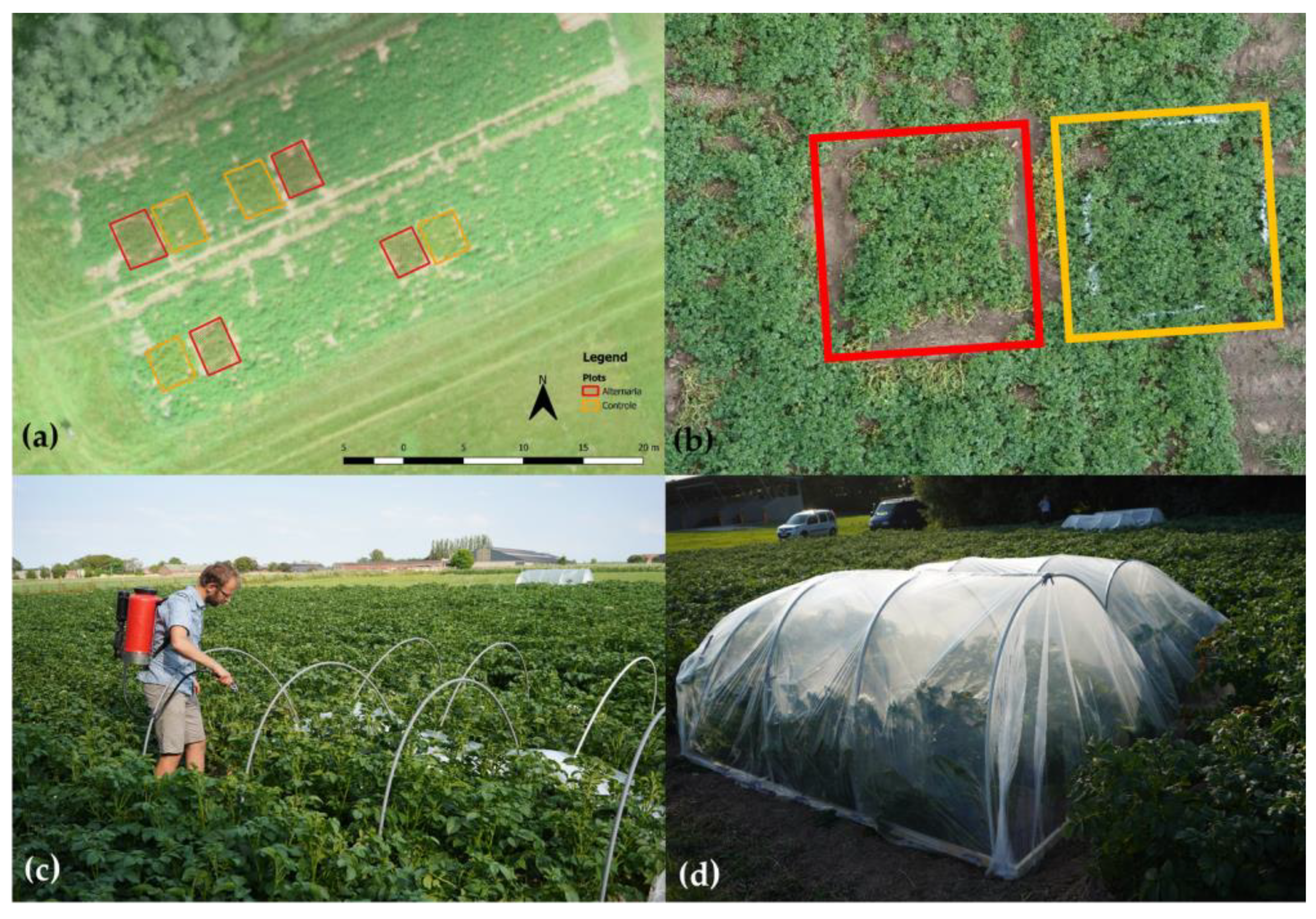
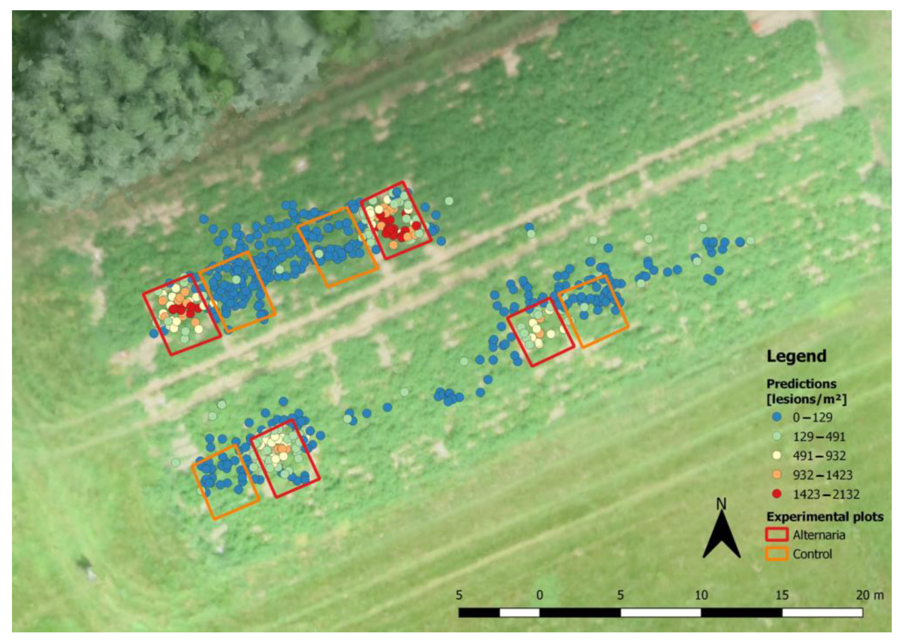
2.1. Field Trials

In order to collect sufficient data for further analysis, a field trial with laboratory-grown inoculum was established [20]. Potato seedlings of cultivar S. tuberosum L. cv. Spunta were planted on 6 May 2019, at an experimental field of 40 × 20 m with a sandy loam soil in Merelbeke, Belgium (50.986544°N, 3.774066°E). The between-row distance was 0.75 m, and the planting distance between the tubers was 0.4 m. After crop closure and flowering, four twin plots were delineated. Each single plot measured 3.4 × 1.8 m and contained 32 plants (4 rows of 8 plants). Per twin plot, one plot was assigned as a control and one as an infected plot. An overview of the field experiment is given in Figure 1, where the red boxes indicate the infected plots and the orange boxes the control plots. Inoculum was produced by growing local field isolates of A. solani on V8 agar plates under near UV light for 10 days. Conidiospores were rinsed off the plates using water with 0.01% Tween, filtered using nylon netting (200 µm), counted with a haemocytometer and diluted to $3\times {10}^3$ spores per mL.

The inoculation was performed on 30 July 2019 in the evening by spraying the plants in the plot homogenously with 400 mL of inoculum using a handheld sprayer (Birchmeier, Stetten, Argau, CHE). To facilitate a sufficiently long period of leaf wetness and promote infection, the plants were covered overnight with a transparent plastic foil and supported by beams of plastic tubing to avoid contact with the plants. Control plots were not sprayed or covered with plastic foil.

The first noticeable symptoms appeared at 3 days after inoculation (DAI); thereafter, the symptoms developed steadily until 14 DAI when the lesion growth ceased. During symptom development, UAV flights were carried out the day before inoculation and at 3, 6, 9, 13 and 15 DAI.

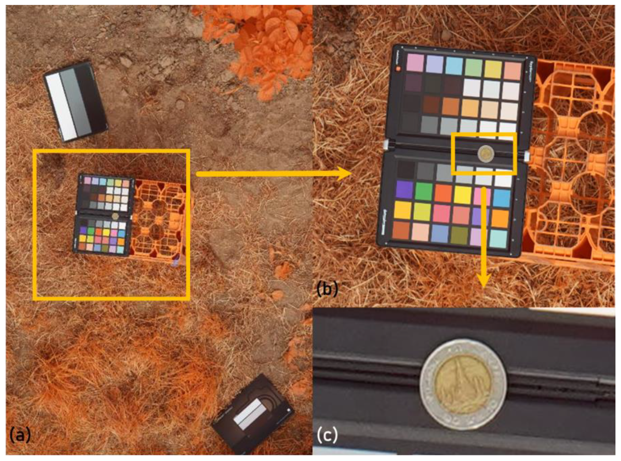
2.2. UAV Flights

The UAV flights were performed with a DJI Matrice 600 (DJI, Shenzhen, Guangdong, CHN) equipped with a Ronin MX gimbal (DJI, Shenzhen, Guangdong, China) and a modified RGB Sony a7R III camera (42.4 MP, mirrorless) (Sony, Minato, Tokyo, Japan), with a 135 mm lens, type Carl Zeiss Batis 135 mm f2.8 (Zeiss, Oberkochen, Baden-Württemberg, Germany). The RGB version of the camera was modified by LifePixel (LifePixel, Seattle, WA, USA) to remove the near-infrared (NIR) blocking filter. This adaptation allowed the red channel of the camera to also capture photons in the NIR range. Previous research showed that higher contrast between healthy and infected tissue can be perceived in the NIR spectrum [20], making the modified RGB camera more appropriate compared to the regular RGB version for this specific use.

At a flying height of 10 m above ground level, ultra-high-resolution images with a field-of-view (FOV) of about 2.7 m × 1.5 m with a resolution of 0.3 mm/px were obtained for disease detection. Due to the relative error of the on-board GNSS system (horizontal hovering accuracy of ±1.5 m) in combination with the flight planning software, DJI Ground Station Pro (DJI, Shenzhen, Guangdong, China), a preprogrammed flight could not guarantee sufficient cover of the plots. Hence, flights were performed manually with the UAV hovering over the plots to allow the acquisition of a sufficiently large number of images of the plots. The cameras recorded an image every second. This resulted in an average number of 60 images per plot.

Additionally, flights at 60 m (FOV of 16 m × 9 m, 1.8 mm/px resolution) above ground level were performed to construct an overview map, for which Agisoft Metashape Professional v1.8 (Agisoft, St. Petersburg, Russian) was used. Nine ground control points (GCPs) were used during the flights and were measured with an RTK-GPS (S10 GNSS Receiver) (Stonex, Paderno Dugnano, Milan, Italy), allowing location measurements to be made at centimetre-level precision. Using these reference measurements, the stitched orthomosaic could also be georeferenced at centimetre-level precision.

To assess the spectral response of this camera, a spyder color checker (Datacolor, Trenton, NJ, USA) was used as spectral reference in the field during the flights. The spectral reference was also measured by an FX10e hyperspectral linescan camera covering the wavelength range from 400 to 1000 nm with an average FWHM (full width at halve maximum, i.e., spectral resolution) of 5.5 nm.

As mentioned in the introduction, high spatial resolution is crucial for disease detection. To verify the resolution, a coin was placed in the images as a reference during each flight. By measuring the coin diameter and the corresponding area in the images, an accurate estimation of the spatial resolution could be obtained. The colour checker and coin were placed on a tray to ensure the resolution was measured around canopy height (Figure 2). The area of the coin in a representative image was recorded and compared with the actual surface of the coin. This confirmed that the image resolution was 0.32 mm/pixel.

2.3. Image Analysis Workflow

The image analysis workflow is illustrated schematically in Figure 3. As a first action in the analysis workflow, the images were labelled using QGIS 3.10 (QGIS Association, Gossau, Zürich, CHE) [34]. For annotation geometry, points placed at the lesion centre were chosen over rectangles or polygons, as annotating rectangles or polygons is more time-consuming and the main objective is the localization of the lesions and the estimation of their size. For this proof of concept, two images of 42 MP (7952 × 5304 pixels), recorded at 5 August 2019 (6 DAI), were randomly selected and annotated with 5465 and 9887 lesions, respectively.

The annotated points (vectors) were then converted into a density map using a kernel density estimation (Equation (1)). Previous research indicated that the use of density maps eases the training process of the CNN by reducing the complexity of predicting the exact location to predict a coarse location [35]. To calculate the density maps, the Python module scikit-learn was used with the values 2, 10, 25 and 100 pixels as bandwidths [36]. The bandwidth defines the area over which the points are averaged. A larger bandwidth will therefore result in a more smoothed approximation. This bandwidth should be chosen in relation to the density of the objects and thus reversely with the size of the objects [37].

The main motivation for using densities (raster) instead of discrete points (vector) is its ease of use during evaluation (regression) and implementation. Moreover, the nature of the problem (counting lesions within a certain area) lies closer to a regression problem than to object detection. In addition, the conversion from points to density maps is often done in deep learning as an in-between step for point detection to guide the network towards the correct coordinates [38,39]. Moreover, models trained to estimate density maps are computationally faster and can be easily converted to additionally produce coordinates when required. As the images and labels were too large to be fed directly to the network, both were subsampled to smaller images 256 × 256 pixels in size.

$$P_{ij}=L_{img}\cdot \frac{1}{\sqrt{2\pi }}{e}^{-d^2/2h^2}$$

(1)

with

• $P_{ij}$: density estimate of lesion occurrence at pixel ij
• $L_{img}$: the number of annotated lesions in the image
• $d$: the distance to the annotated lesion
• $h$: the bandwidth of the kernel density estimation

In Figure 4a, the frequency distributions of Alternaria solani lesions are compared between the two labelled images. Clearly, the longer tail for one image (DSC06979) indicates the higher density of annotations. It should be noted that similar concentrations of Alternaria solani lesions can be expected for both images, but the slightly lower sharpness in image DSC07392 resulted in a lower visibility of the symptoms. A comparison between the number of lesions and the approximation by a kernel density function for the two images is illustrated in Figure 4b,c. An identity line is plotted to ease comparison. For tiles with a low lesion count, the kernel density approximate tends to overestimate, while for higher occurrences, underestimation can be noted. It is clear that for higher bandwidths, this effect is worse than for smaller bandwidths. This is also in line with Zhang et al., 2016, who indicated that the optimal bandwidth is related to the size of the objects [37]. Therefore, a bandwidth of 2 pixels was used to train the model.

Three different datasets were constructed: a training dataset to train the model, a validation dataset for hyperparameter tuning and finally an independent test dataset for assessing model performance. The validation dataset was constructed by randomly taking 186 tiles of 256 × 256 pixels from the two annotated images. After sampling, these tiles were removed from the original images. Then, the training set of 744 tiles was randomly subsampled during model training as a data augmentation technique so that no tiles were exactly the same. Occasionally, training tiles were picked with overlap where the validation tiles were removed, resulting in partially occluded training tiles. To ensure a good quality of the training set (i.e., the images contained enough nonempty regions), only tiles that had a less than 25% overlap (occlusion) with previously sampled tiles were selected.

The independent test set was randomly sampled separately from the remaining UAV images, and the selected tiles were annotated. This resulted in a test set of 320 image tiles. By comparing the distributions of Alternaria solani occurrences in the test and training set (Figure 5), it was confirmed that the training set was similar to the test set and therefore representative for the whole dataset.

Prior to image analysis, the images were normalized by subtracting the mean colour value and dividing by the standard deviation of the colour bands. This standardization was applied to both the images and the labels based on statistics derived from the training set (

Table 1. Image and density map statistics used for the standardization.

	Red	Green	Blue	Density Map
Mean	0.72	0.27	0.079	0.00020
Standard deviation	0.22	0.12	0.063	0.00051

). It was shown in earlier research that standardization has a positive impact on the learning speed [40]. This can be explained by the centring of values around zero, thereby minimizing imbalances in the pixel values that could result in exploding gradients.

As model architecture, a segmentation model was chosen to allow pixel-based regression. U-Net is a well-established segmentation model [41,42,43,44]. This architecture was used with a ResNet-50 backbone and one output layer, as only one class probability needed to be predicted [45]. A linear activation function of the output layer allows linear regression estimations of per-pixel probabilities of disease occurrence, computed trough the kernel density estimation. Initial weights trained on ImageNet were used. As the mean squared error (MSE, Equation (2)) is commonly used as a performance measure in regression, this was also applied here as the loss function. Adam was used as the optimizer with a learning rate of ${10}^{-3}$. The models were trained using Python 3.8 (Python Software Foundation, Fredericksburg, VA, USA), Tensorflow 2.5 (Google Brain, Mountain View, CA, USA) and the Segmentation Models package [46,47,48].

$$MSE=\frac{1}{n}{{\displaystyle \sum }}_{i=0}^n{\left(y_i-{y_i}^p\right)}^2$$

(2)

with:

• $n$: the number of pixels in an image
• $y_i$: the ground truth value for the i-th pixel
• ${y_i}^p$: the predicted value for the i-th pixel

A batch size of 8 images was used during training as a trade-off between GPU memory (GTX 1080, 8 GB RAM) (NVIDIA, Santa Clara, CA, USA) and training speed. The model was trained for 100 epochs while the loss function was monitored to verify that the training converged.

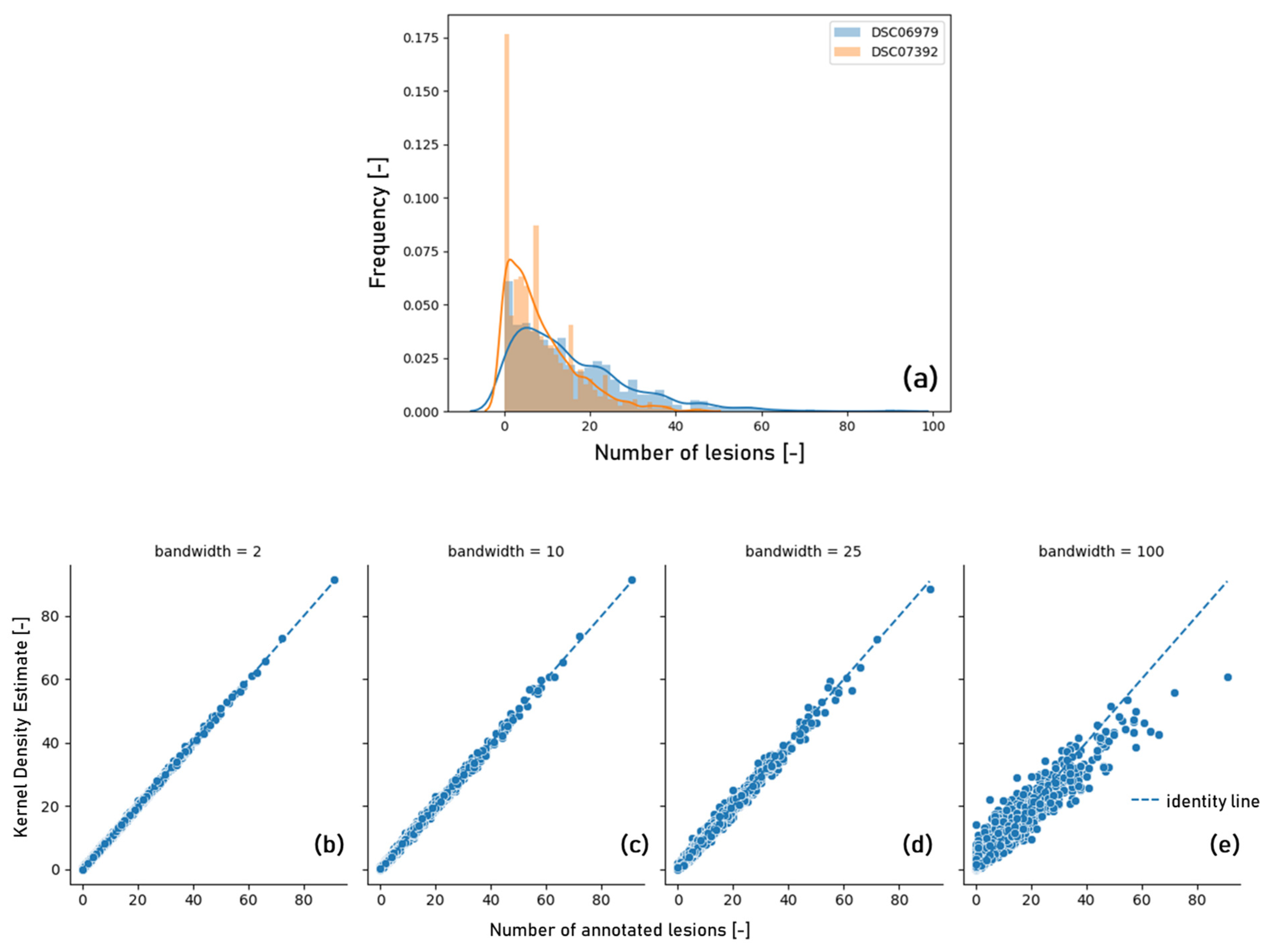
3. Results

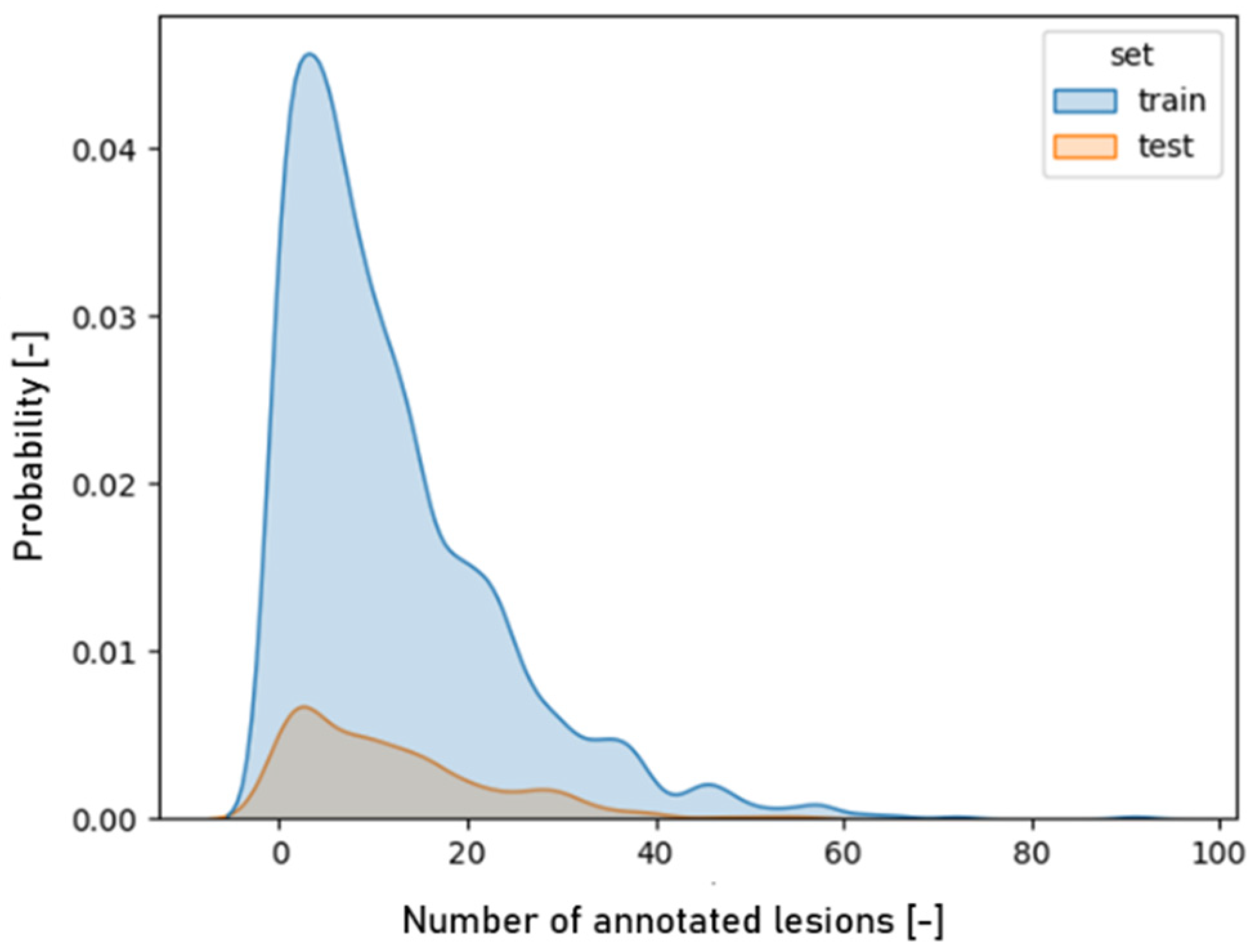
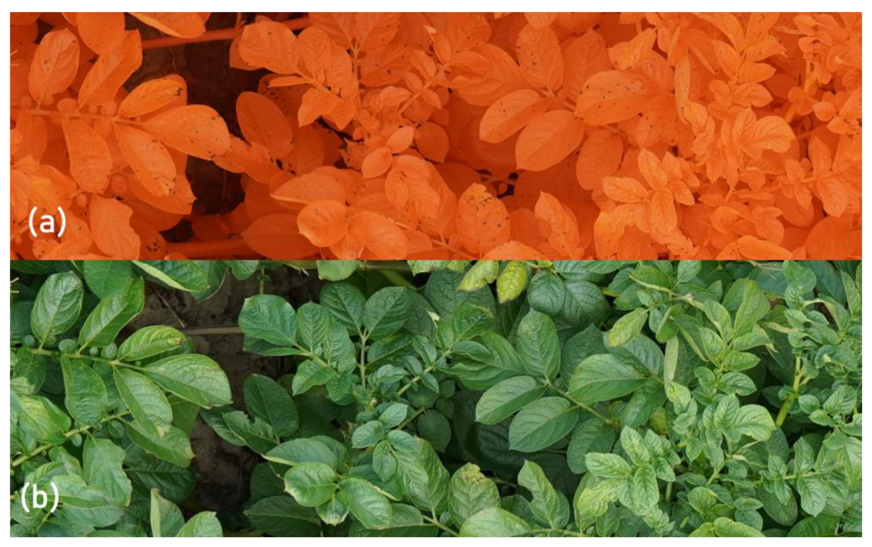
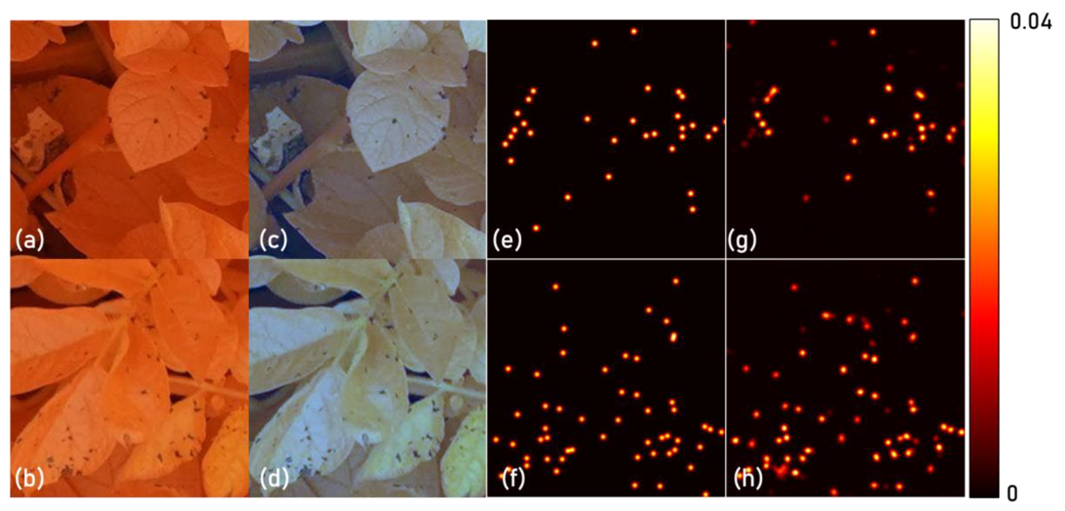
3.1. Image Characteristics

Figure 6 shows a section of a normal RGB image (also acquired with a Sony a7R III and the 135 mm lens on the UAV at the same 10 m flight height) and a modified RGB image. Both images were taken at the same day (5 August 2019, 6 DAI) over the same area.

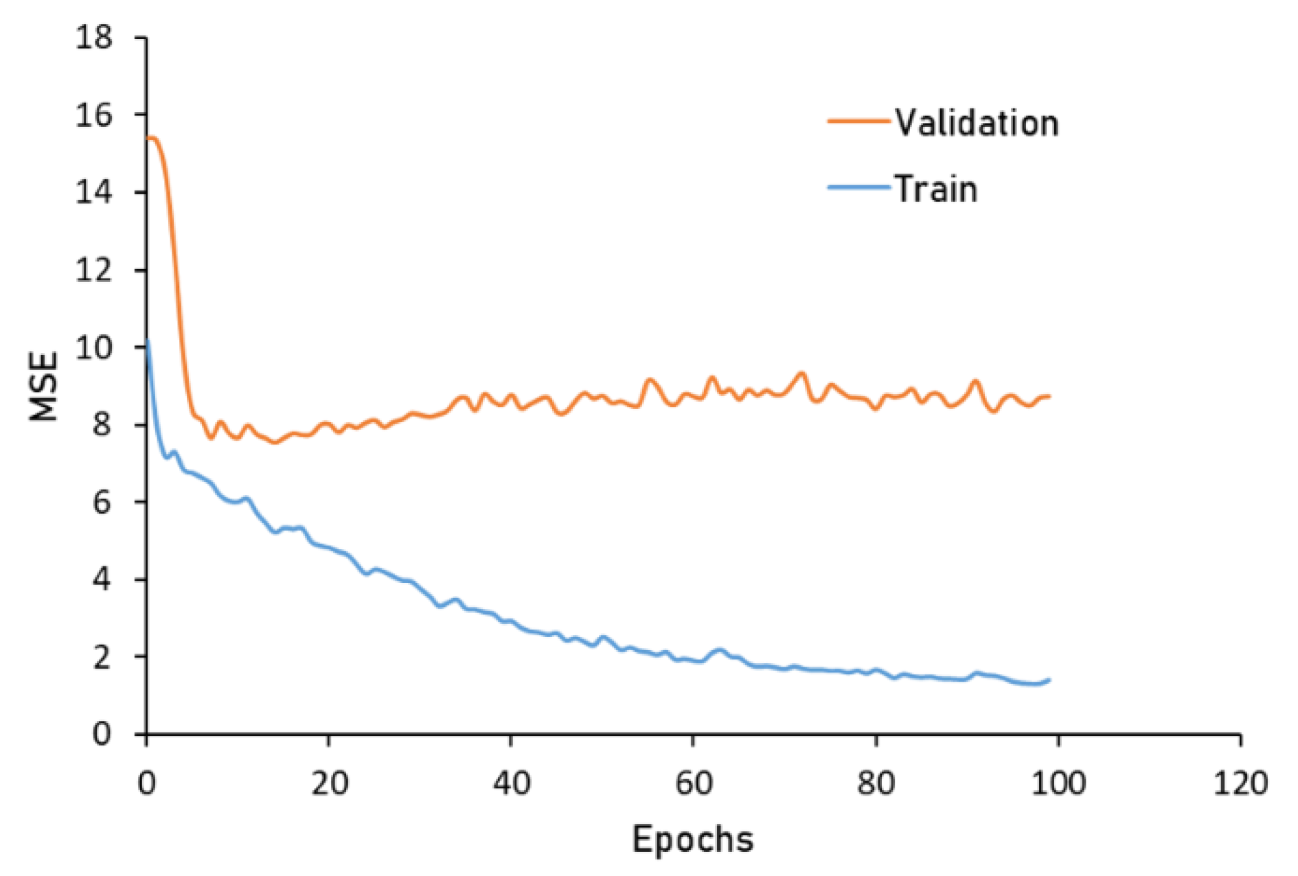
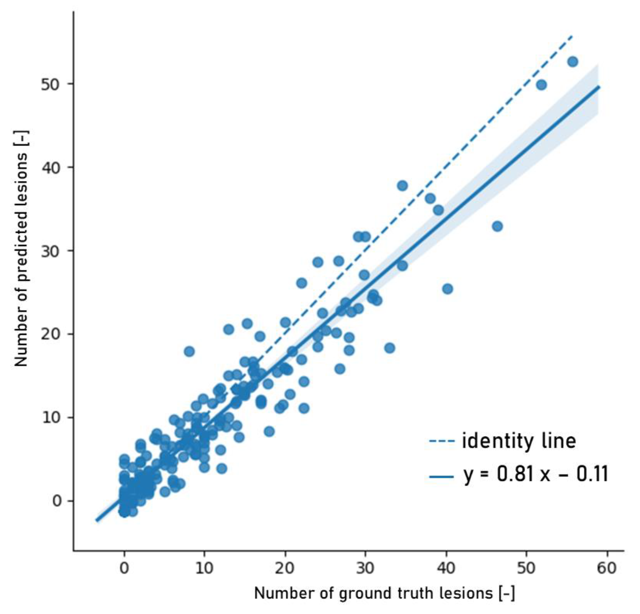
3.2. Model Analysis

During preprocessing, the standardization of the tiles clearly enhanced the contrast between lesions and unaffected leaf areas (Figure 7). The validation loss converged after 15 epochs (Figure 8). This indicates that the model learns the required features very quickly.

In Figure 9, the performance of the detection algorithm is illustrated via the plotting of the number of detected lesions per tile against the corresponding kernel density estimation based on annotated lesions. The R² of 0.96 indicates a very good lesion counting performance. However, the slope of 0.81 and negative intercept of −0.11 suggest that the model underestimates the true number of lesions in a tile.

In Figure 10, the detection performance of the U-Net is illustrated for a number of representative image tiles. The network accurately detected most lesions and sometimes even performed better than did the labeller, finding lesions that the labeller had missed (Figure 10a). Note also the fly in the modified RGB image (white arrow). The model was slightly triggered, but was able to accurately distinguish Alternaria solani lesions from the fly.

Figure 10b,c show regions where the model falsely indicates lesions (false positives) or misses lesions (false negatives), respectively. In Figure 10b, the large size of the lesions is uncommon and causes confusion, resulting in a lower confidence score and a false negative. In Figure 10c, the leaf axils look very similar to lesions having a small size and clear borders while being surrounded by healthy tissue. While a human labeller takes the leaf and stem branch into account, the model clearly failed to take this larger context into account. This is a difficulty already noted in previous research [49,50], where small objects were still often missed due to (1) the absolute size of the object providing less information for the network to classify the object correctly and (2) the mismatch in receptor head and the object size. This was solved respectively by (1) providing more detail to the network by additionally sampling the earlier feature maps [51,52] or incorporating both local and global context [53] and (2) maintaining higher spatial resolution in the deeper layers [54].

It was also noted that the centre of the lesions is often predicted a few pixels away from the ground truth annotation. This might be attributed to small inaccuracies in the labelling.

During image acquisition, the drone was manually flown with the camera triggering every second. This strategy resulted in a large dataset of 672 high-resolution images of infected zones as well as healthy zones. By applying the trained model to all images, geographical estimates of infection pressure could be calculated, which are illustrated in Figure 11. It can be seen that the noninfected plots (orange rectangles) and the rest of the field are clearly distinguishable from the infected plots. The infected plots show higher numbers of lesions at their centres compared to the border regions. This can be attributed to the size of the images (2.7 × 1.5 m), which overlaps almost completely with a plot. This implies that images taken at the border of an infected plot contain both infected plants as well as noninfected plants surrounding the plot. The large coverage of the image therefore has a spatial smoothing effect.

A number of lesions were predicted in every image regardless of the actual location or presence of Alternaria solani. As the field is amply sampled with images, these points give an accurate measure of infection hotspots (Figure 12). In order to obtain this density map, ordinary kriging was used as interpolation technique [55]. Typically, the interpolated infection map is obtained at high spatial resolution (10 cm/px) as a detailed guide for the farmer to locate potential sources of infection. By grouping and averaging neighbouring pixels, a lower resolution application map (1 m/px) is generated, specifically designed to fit the farmer’s spraying machine. This will allow a farmer to adjust the protection measures according to the infection pressure and could lead to a reduction in pesticide use and a higher degree of protection.

4. Discussion

4.1. Image Characteristics

It can be seen that the increased sensitivity to the NIR region enhances the contrast between the Alternaria solani-induced lesions, visible as dark spots on the leaves, and the unaffected zones on the leaves. In addition, the wax layer on the leaves introduces glare in the RGB images reducing the contrast, whereas the modified RGB images display less specular reflectance, further increasing the image contrast.

4.2. Model Analysis

It should also be noted that the model is still prone to under- and overestimations. In addition, the green points in Figure 11 show a slightly elevated lesion density (green dots) even though they are also outside the infected plots. These false positives can be linked to leaf axils, earth or other brown spots, or even flies on the leaves (Figure 10a). To reduce these false positives, it is recommended to train the model on real-world datasets, with more healthy plants compared to Alternaria solani-infected plants and thus an in-field occurring class imbalance.

The minimal lesion density threshold that can be detected by the model should also be investigated. As the model outputs per-pixel probabilities (regression) rather than classes, there will always be base noise, linked to the limit of detection of the model. Extending the training dataset with other potato varieties, fields and illumination conditions will enhance the model robustness and further decrease the limit of detection. Estimating this threshold will be essential (and nontrivial) for its final application, as farmers would want to detect a disease outbreak as early as possible (when only few lesions are present).

It should be noted that in a first stage, the maps will be a guide for the farmers to show them which zones in the field to check. The farmer will still have to make the final decision whether the model estimates are correct or require adjustments.

Further research might focus on implementing state-of-the-art point detection models such as CenterNet [39] and the one developed by [38]. In addition, even though the labelling effort was minimal owing to the pointwise detections, it could be interesting to investigate alternative approaches, such as classification based on the subtiles of a UAV image to further reduce the labelling effort and lower the burden to retrain AI models.

In addition, future research should investigate the impact of UAV flight velocity and camera settings, such as diaphragm, shutter speed and ISO value, on the model accuracy, as it was seen that at high velocity segments, images were blurred and a larger number of false positives occurred.

Automating the workflow will be key to adoption by farmers. In this study, expert knowledge about the UAV, camera, lens and gimbal was still required to operate the UAV successfully. A small UAV with an integrated high-resolution camera, possibly with near real-time processing in the cloud through 5G data streaming could substantially increase the applicability, as it would allow the farmer to use the result immediately after the flight as an input for precision crop protection.

The demonstrated methodology can be transferred to other plant–pathogen interactions, with the main challenge being collecting and accurately annotating the disease symptoms. This is especially relevant for disease detection, where a pronounced class imbalance requires the collection and annotation of a sufficiently large training dataset. Future work will include the detection of Phytophthora infestans due to its notorious economic impact on potato production.

Extending the methodology towards correctly classifying different diseases at the same crop might be challenging, as differentiating symptoms often requires fine detail and expert knowledge. It should therefore be further investigated if the used spatial resolution (0.3 mm/px) is sufficient for classifying multiple diseases. This methodology should therefore initially be used as a guide for a process in which the farmers are decision makers.

From an economic perspective, mapping multiple plant–pathogen interactions will increase the profitability of a UAV platform for the farmer. This might be catalysed by regulated drone-in-a-box solutions, where consecutive flights will become relatively cheap and might discover several anomalies in the farmers’ fields. In a first stage, the farmer will be able to act in a timelier fashion and reduce the disease impact. In a later stage, when the detection method is extremely accurate and curative crop protection products are highly efficient, this methodology might even enable site-specific spraying of infected plants.

5. Conclusions

A workflow was created to map the spread of Alternaria solani infection in potato fields based on UAV imaging. Modified RGB imaging was used to provide enhanced contrast between Alternaria solani lesions and unaffected tissue. In combination with the state-of-the-art spatial resolution that can be obtained using consumer cameras, this modified RGB camera was found to be ideally suited for UAV-based disease detection. Ultra-high -resolution images were captured with a spatial resolution of 0.3 mm/pixel, crucial for the detection of Alternaria solani–induced lesions on potato leaves. We demonstrated how combination of this ultra-high-resolution imagery with deep learning can promote precision crop protection.

A segmentation network (U-Net) was trained to estimate the probability of disease presence by counting the number of lesions in an image. Even though the size of the training dataset was limited, the model proved to be very accurate on the leaf level. When extrapolated towards the field scale, prediction errors were found to accumulate, raising the detection limit of the model.

References

- FAO. Food and Agriculture Organization of the United Nations. 2022. Available online: https://www.fao.org/faostat/en/#home. (accessed on 20 November 2022).
- Horsfield, A.; Wicks, T.; Davies, K.; Wilson, D.; Paton, S. Effect of fungicide use strategies on the control of early blight (Alternaria solani) and potato yield. Australas. Plant Pathol. 2010, 39, 368–375. [Google Scholar] [CrossRef]
- Harrison, M.D.; Venette, J.R. Chemical control of potato early blight and its effect on potato yield. Am. Potato J. 1970, 47, 81–86. [Google Scholar] [CrossRef]
- Van der Waals, J.E.; Korsten, L.; Aveling, T.A.S. A review of early blight of potato. Afr. Plant Prot. 2001, 7, 91–102. [Google Scholar]
- Tsedaley, B. Review on early blight (Alternaria spp.) of potato disease and its management options. J. Biol. Agric. Healthc. 2014, 4, 191–199. [Google Scholar] [CrossRef] [Green Version]
- Leiminger, J.; Hausladen, H. Early blight: Influence of different varieties. PPO-Spec. Rep. 2007, 12, 195–203. [Google Scholar]
- American Phytopathological Society; Potato Association of America. Compendium of Potato Diseases; Hooker, W.J., Ed.; American Phytopathological Society: Saint Paul, MN, USA, 1981; ISBN 0890540276. [Google Scholar]
- Nasr-Esfahani, M. An IPM plan for early blight disease of potato Alternaria solani sorauer and A. alternata (Fries.) Keissler. Arch. Phytopathol. Plant Prot. 2020, 55, 785–796. [Google Scholar] [CrossRef]
- Zhang, N.; Yang, G.; Pan, Y.; Yang, X.; Chen, L.; Zhao, C. A review of advanced technologies and development for hyperspectral-based plant disease detection in the past three decades. Remote Sens. 2020, 12, 3188. [Google Scholar] [CrossRef]
- Mahlein, A. Present and Future Trends in Plant Disease Detection. Plant Dis. 2016, 100, 241–251. [Google Scholar] [CrossRef] [Green Version]
- Mahlein, A.; Kuska, M.T.; Behmann, J.; Polder, G.; Walter, A. Hyperspectral Sensors and Imaging Technologies in Phytopathology: State of the Art. Annu. Rev. Phytopathol. 2018, 56, 535–558. [Google Scholar] [CrossRef]
- Zhang, J.; Huang, Y.; Pu, R.; Gonzalez-moreno, P.; Yuan, L. Monitoring plant diseases and pests through remote sensing technology: A review. Comput. Electron. Agric. 2019, 165, 104943. [Google Scholar] [CrossRef]
- Tetila, E.C.; Machado, B.B.; Menezes, G.K.; Oliveira, S.; Alvarez, M.; Amorim, W.P.; Alessandro, N.; Belete, D.S.; Gonçalves, G.; Pistori, H. Automatic Recognition of Soybean Leaf Diseases Using UAV Images and Deep Convolutional Neural Networks. IEEE Geosci. Remote Sens. Lett. 2019, 17, 903–907. [Google Scholar] [CrossRef]
- Zhang, X.; Han, L.; Dong, Y.; Shi, Y.; Huang, W.; Han, L.; González-Moreno, P.; Ma, H.; Ye, H.; Sobeih, T. A deep learning-based approach for automated yellow rust disease detection from high-resolution hyperspectral UAV images. Remote Sens. 2019, 11, 1554. [Google Scholar] [CrossRef]
- Maes, W.H.; Steppe, K. Perspectives for Remote Sensing with Unmanned Aerial Vehicles in Precision Agriculture. Trends Plant Sci. 2019, 24, 152–164. [Google Scholar] [CrossRef] [PubMed]
- Dehkordi, R.H.; EL JARROUDI, M.; Kouadio, L.; Meersmans, J.; Beyer, M. Monitoring wheat leaf rust and stripe rust in winter wheat using high-resolution uav-based red-green-blue imagery. Remote Sens. 2020, 12, 3696. [Google Scholar] [CrossRef]
- Wiesner-Hanks, T.; Wu, H.; Stewart, E.; DeChant, C.; Kaczmar, N.; Lipson, H.; Gore, M.A.; Nelson, R.J. Millimeter-Level Plant Disease Detection From Aerial Photographs via Deep Learning and Crowdsourced Data. Front. Plant Sci. 2019, 10, 1550. [Google Scholar] [CrossRef] [Green Version]
- Singh, A.P.; Yerudkar, A.; Mariani, V.; Iannelli, L.; Glielmo, L. A Bibliometric Review of the Use of Unmanned Aerial Vehicles in Precision Agriculture and Precision Viticulture for Sensing Applications. Remote Sens. 2022, 14, 1604. [Google Scholar] [CrossRef]
- Shafi, U.; Mumtaz, R.; García-nieto, J.; Hassan, S.A.; Zaidi, S.A.; Iqbal, N. Precision Agriculture Techniques and Practices: From consideration to application. Sensors 2019, 19, 3796. [Google Scholar] [CrossRef] [Green Version]
- Van De Vijver, R.; Mertens, K.; Heungens, K.; Somers, B.; Nuyttens, D.; Borra-serrano, I.; Lootens, P.; Roldán-ruiz, I.; Vangeyte, J.; Saeys, W. In-field detection of Alternaria solani in potato crops using hyperspectral imaging. Comput. Electron. Agric. 2020, 168, 105106. [Google Scholar] [CrossRef]
- Dutta, K.; Talukdar, D.; Bora, S.S. Segmentation of unhealthy leaves in cruciferous crops for early disease detection using vegetative indices and Otsu thresholding of aerial images. Measurement 2022, 189, 110478. [Google Scholar] [CrossRef]
- Mohanty, S.P.; Hughes, D.P.; Salathé, M. Using Deep Learning for Image-Based Plant Disease Detection. Front. Plant Sci. 2016, 7, 1419. [Google Scholar] [CrossRef] [Green Version]
- Ferentinos, K.P. Deep learning models for plant disease detection and diagnosis. Comput. Electron. Agric. 2018, 145, 311–318. [Google Scholar] [CrossRef]
- Singh, D.; Jain, N.; Jain, P.; Kayal, P.; Kumawat, S.; Batra, N. PlantDoc: A dataset for visual plant disease detection. In Proceedings of the 7th ACM IKDD CoDS and 25th COMAD, Hyderabad, India, 5–7 January 2020; pp. 249–253. [Google Scholar] [CrossRef]
- Saleem, M.H.; Potgieter, J.; Arif, K.M. Plant disease detection and classification by deep learning. Plants 2019, 8, 32–34. [Google Scholar] [CrossRef] [PubMed] [Green Version]
- Roy, A.M.; Bhaduri, J. A Deep Learning Enabled Multi-Class Plant Disease Detection Model Based on Computer Vision. Ai 2021, 2, 413–428. [Google Scholar] [CrossRef]
- Arsenovic, M.; Karanovic, M.; Sladojevic, S.; Anderla, A.; Stefanovic, D. Solving current limitations of deep learning based approaches for plant disease detection. Symmetry 2019, 11, 939. [Google Scholar] [CrossRef] [Green Version]
- Arnal Barbedo, J.G. Plant disease identification from individual lesions and spots using deep learning. Biosyst. Eng. 2019, 180, 96–107. [Google Scholar] [CrossRef]
- Kattenborn, T.; Eichel, J.; Fassnacht, F.E. Convolutional Neural Networks enable efficient, accurate and fine-grained segmentation of plant species and communities from high-resolution UAV imagery. Sci. Rep. 2019, 9, 17656. [Google Scholar] [CrossRef] [Green Version]
- Krizhevsky, A.; Sutskever, I.; Hinton, G.E. ImageNet Classification with Deep Convolutional Neural Networks. In Proceedings of the Neural Information Processing Systems, Lake Tahoe, NV, USA, 3–6 December 2012; pp. 1106–1114. [Google Scholar]
- LeCun, Y.; Bengio, Y.; Hinton, G. Deep learning. Nature 2015, 521, 436–444. [Google Scholar] [CrossRef]
- Singh, A.K.; Ganapathysubramanian, B.; Sarkar, S.; Singh, A. Deep Learning for Plant Stress Phenotyping: Trends and Future Perspectives Machine Learning in Plant Science. Trends Plant Sci. 2018, 23, 883–898. [Google Scholar] [CrossRef] [Green Version]
- Bouguettaya, A.; Zarzour, H.; Kechida, A.; Taberkit, A.M. Deep learning techniques to classify agricultural crops through UAV imagery: A review. Neural Comput. Appl. 2022, 34, 9511–9536. [Google Scholar] [CrossRef]
- QGIS Development Team. QGIS Geographic Information System 2019. Available online: https://qgis.org (accessed on 20 November 2022).
- Sam, D.B.; Surya, S.; Babu, R.V. Switching Convolutional Neural Network for Crowd Counting. In Proceedings of the IEEE Conference on Computer Vision and Pattern Recognition (CVPR), Honolulu, HI, USA, 21–26 July 2017; pp. 5744–5752. [Google Scholar] [CrossRef] [Green Version]
- Pedregosa, F.; Michel, V.; Grisel, O.; Blondel, M.; Prettenhofer, P.; Weiss, R.; Vanderplas, J.; Cournapeau, D.; Pedregosa, F.; Varoquaux, G.; et al. Scikit-learn: Machine learning in python. J. Mach. Learn. Res. 2011, 12, 2825–2830. [Google Scholar]
- Zhang, Y.; Zhou, D.; Chen, S.; Gao, S.; Ma, Y. Single-image Crowd Counting via Multi-column Convolutional Neural Network. In Proceedings of the IEEE Conference on Computer Vision and Pattern Recognition (CVPR), Las Vegas, NV, USA, 27–30 June 2016; pp. 589–597. [Google Scholar] [CrossRef]
- Ribera, J.; David, G.; Chen, Y.; Delp, E.J. Locating Objects Without Bounding Boxes. In Proceedings of the IEEE/CVF Conference on Computer Vision and Pattern Recognition (CVPR), Long Beach, CA, USA, 15–20 June 2019; pp. 6479–6489. [Google Scholar]
- Zhou, X.; Wang, D.; Krähenbühl, P. Objects as Points. arXiv 2019, arXiv:1904.07850. [Google Scholar]
- Shorten, C.; Khoshgoftaar, T.M. A survey on Image Data Augmentation for Deep Learning. J. Big Data 2019, 6, 60. [Google Scholar] [CrossRef]
- Ronneberger, O.; Fischer, P.; Brox, T. U-Net: Convolutional Networks for Biomedical Image Segmentation. In Proceedings of the Medical Image Computing and Computer-Assisted Intervention—MICCAI 2015, Munich, Germany, 5–9 October 2015; pp. 234–241. [Google Scholar] [CrossRef] [Green Version]
- Zhao, X.; Yuan, Y.; Song, M.; Ding, Y.; Lin, F.; Liang, D. Use of Unmanned Aerial Vehicle Imagery and Deep Learning UNet to Extract Rice Lodging. Sensors 2019, 19, 3859. [Google Scholar] [CrossRef] [PubMed] [Green Version]
- Zou, K.; Chen, X.; Zhang, F.; Zhou, H.; Zhang, C. A field weed density evaluation method based on uav imaging and modified u-net. Remote Sens. 2021, 13, 310. [Google Scholar] [CrossRef]
- Wang, C.; Du, P.; Wu, H.; Li, J.; Zhao, C.; Zhu, H. A cucumber leaf disease severity classification method based on the fusion of DeepLabV3+ and U-Net. Comput. Electron. Agric. 2021, 189, 106373. [Google Scholar] [CrossRef]
- He, K.; Zhang, X.; Ren, S.; Sun, J. Deep residual learning for image recognition. In Proceedings of the 2016 IEEE Conference on Computer Vision and Pattern Recognition (CVPR), Las Vegas, NV, USA, 27–30 June 2016; pp. 770–778. [Google Scholar] [CrossRef] [Green Version]
- Yakubovskiy, P. Segmentation Models. In GitHub Repository; GitHub: San Francisco, CA, USA, 2019. [Google Scholar]
- Chollet, F. Keras; GitHub: San Francisco, CA, USA, 2015. [Google Scholar]
- Abadi, M.; Agarwal, A.; Barham, P.; Brevdo, E.; Chen, Z.; Citro, C.; Corrado, G.S.; Davis, A.; Dean, J.; Devin, M.; et al. TensorFlow: Large-Scale Machine Learning on Heterogeneous Systems. arXiv 2015, arXiv:1603.04467. [Google Scholar]
- Tong, K.; Wu, Y.; Zhou, F. Recent advances in small object detection based on deep learning: A review. Image Vis. Comput. 2020, 97, 103910. [Google Scholar] [CrossRef]
- Wang, X.; Zhu, D.; Yan, Y. Towards Efficient Detection for Small Objects via Attention-Guided Detection Network and Data Augmentation. Sensors 2022, 22, 7663. [Google Scholar] [CrossRef]
- Liu, W.; Anguelov, D.; Erhan, D.; Szegedy, C.; Reed, S.; Fu, C.Y.; Berg, A.C. SSD: Single shot multibox detector. In Proceedings of the 14th European Conference on Computer Vision, Amsterdam, The Netherlands, 11–14 October 2016; pp. 21–37. [Google Scholar] [CrossRef] [Green Version]
- Deng, Z.; Sun, H.; Zhou, S.; Zhao, J.; Lei, L.; Zou, H. Multi-scale object detection in remote sensing imagery with convolutional neural networks. ISPRS J. Photogramm. Remote Sens. 2018, 145, 3–22. [Google Scholar] [CrossRef]
- Li, J.; Wei, Y.; Liang, X.; Dong, J.; Xu, T. Attentive Contexts for Object Detection. IEEE Trans. Multimed. 2016, 19, 944–954. [Google Scholar] [CrossRef] [Green Version]
- Li, Z.; Peng, C.; Yu, G.; Zhang, X.; Deng, Y.; Sun, J. DetNet: A Backbone network for Object. arXiv 2018, arXiv:1804.06215. [Google Scholar]
- Wackernagel, H. Ordinary Kriging. In Multivar. Geostatistics; Springer: Berlin/Heidelberg, Germany, 2003; pp. 79–88. [Google Scholar] [CrossRef]