
UAV and GPR Data Integration in Glacier Geometry Reconstruction: A Case Study from Irenebreen, Svalbard


1
Faculty of Geography and Earth Sciences, University of Latvia, LV1586 Riga, Latvia
2
Faculty of Earth Sciences and Spatial Management, Department of Hydrology and Water Management, Polar Research Center, Nicolaus Copernicus University in Toruń, Lwowska 1, 87-100 Toruń, Poland
*
Author to whom correspondence should be addressed.
Remote Sens. 2022, 14(3), 456; https://doi.org/10.3390/rs14030456
Submission received: 23 December 2021
/
Revised: 13 January 2022
/
Accepted: 14 January 2022
/
Published: 19 January 2022
(This article belongs to the Special Issue Advanced Ground Penetrating Radar Theory and Applications II)
Abstract
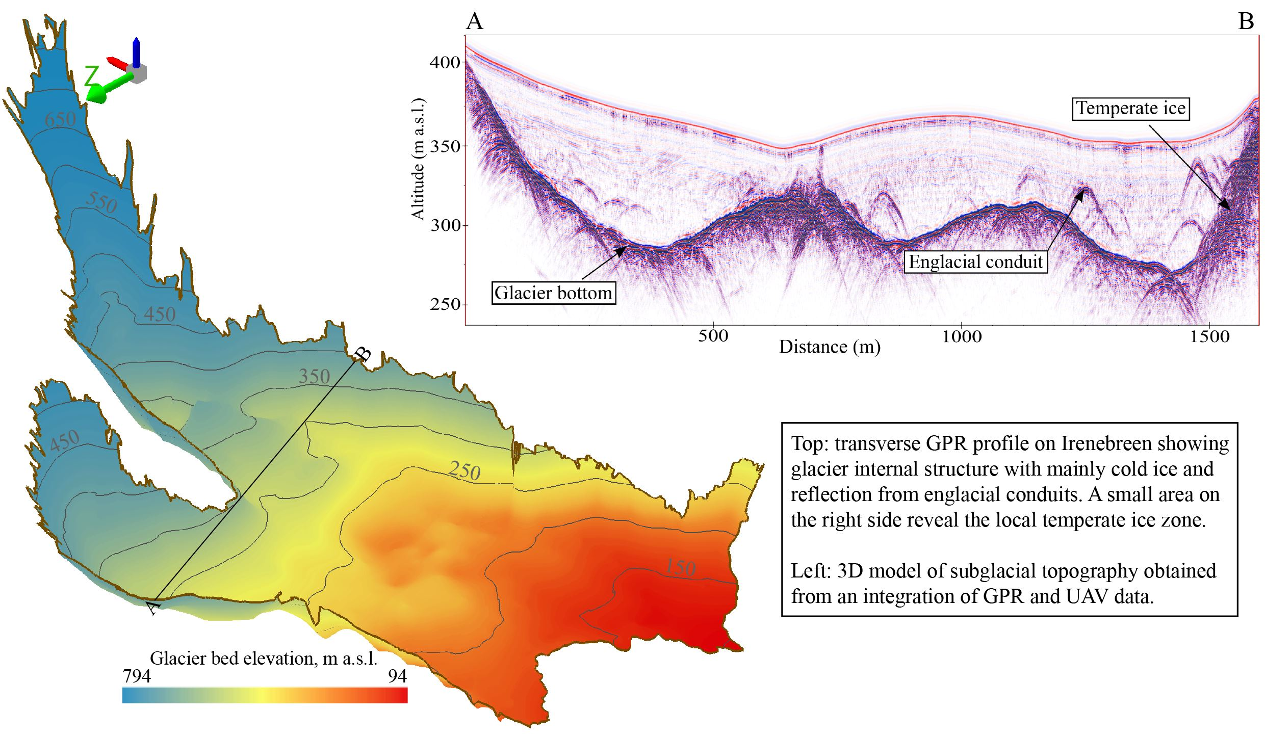
:Although measurements of thickness and internal structure of glaciers are substantial for the understanding of their evolution and response to climate change, detailed data about polythermal glaciers, are scarce. Here, we present the first ground-penetrating radar (GPR) measurement data of Irenebreen, and high-resolution DEM and orthomosaic, obtained from unmanned aerial vehicle (UAV) photogrammetry. A combination of GPR and UAV data allowed for the reconstruction of the glacier geometry including thermal structure. We compare different methods of GPR signal propagation speed determination and argue that a common midpoint method (CMP) should be used if possible. Our observations reveal that Irenebreen is a polythermal glacier with a basal temperate ice layer, the volume of which volume reaches only 12% of the total glacier volume. We also observe the intense GPR signal scattering in two small zones in the ablation area and suggest that intense water percolation occurs in these places creating local areas of temperate ice. This finding emphasizes the possible formation of localised temperate ice zones in polythermal glaciers due to the coincidence of several factors. Our study demonstrates that a combination of UAV photogrammetry and GPR can be successfully applied and should be used for the high-resolution reconstruction of 3D geometries of small glaciers.

1. Introduction
For the understanding of thermal regime, dynamics and following response to climate change, detailed data about the internal structure, volume, and distribution of temperate ice in polythermal glaciers are necessary [1]. It is especially crucial to determine glacier volume as precisely as possible, especially when small glaciers are considered [2,3]. Despite the long history of glacier studies in Svalbard, measurements of ice thickness of individual glaciers with geophysical methods or drillings are still scarce [4,5,6,7], etc., due to the remote location of the archipelago. The same can be stated about the determination of the distribution of cold and temperate ice [5,6,7], etc.
For the determination of precise glacier volume, it is important to obtain a high-resolution digital elevation model (DEM). In cases when large areas are studied, usually data from satellite sensors, aerial photographs or even digitised topographic maps are used ([8], pp. 14–27), [9,10]. When individual glaciers are considered, also GNSS measurements of the glacier surface elevation [11] and LiDAR data [3,12,13] are used; however, the acquisition of LiDAR data can be time-consuming, logistically challenging, and requires expensive equipment with related transportation costs to the areas of high altitude. In the recent decade, an increase in glacier surface DEMs obtained via photogrammetric processing of aerial photographs obtained by UAVs can be observed [14,15,16,17,18,19,20,21,22].
Various remote sensing methods are used for glacier volume and internal structure investigation (for review refer to [23]). Particularly detailed information about glacier internal structure can be obtained using ground-penetrating radar (GPR). Since the first attempts to apply GPR to glacier studies [24] (pp. 4–6), a range of its application has been found [3,4,7,14,25,26,27]. Observing that water inclusions in temperate ice causes intense scattering of GPR signal [5,6,28] provided a powerful tool for detailed mapping of thermal structure of glaciers.
In this paper, we present a case study where data obtained with GPR and UAV are used to create a high-resolution geometry model of a polythermal glacier located in north-western Svalbard. The aim of this study is to demonstrate that UAV and GPR data integration are the most optimal method today for the characterisation of small glacier geometry including the ice surface and bed topography, ice thickness and thermal structure. New data allows us to reveal the volume of the glacier, and temperate ice as well. We discuss the issue of measurements of GPR signal propagation speed, which are crucial for both cold and temperate ice, if a high-resolution geometry of the glacier must be acquired.
2. Study Area
Our study area is located at Kaffiøyra region on Oscar II Land in north-western Spitsbergen. It covers an area of 2582 km2, 70% of which is represented by glaciers, stretching across nearly 1600 km2. The glacierised area consist of ice plateaux with land-terminating valley glaciers bordered by two larger tide-water glaciers [29]. Irenebreen is a valley glacier to the south of Waldemarbreen and is bordered by the Kristinefjella and Gråfjellet mountains to the north. The area of Irenebreen totals 2.90 km2 [30]. Irenebreen has two major accumulation basins—northern and southern cirque (Figure 1a,b). The surface of the glacier is uneven and reveals a substantial cross-sectional asymmetry to the south [31].
The glacier snout is situated at approximately 150 m a.s.l. on average, whereas its southern accumulation basin (cirque) reaches more than 700 m a.s.l. The greatest altitude increase occurs on the glacier snout up to about 300 m a.s.l., and, above that—up to 400 m a.s.l.—the glacier surface becomes almost flat. The northern accumulation basin (cirque) is situated lower than the southern one and its largest area is at 400–450 m a.s.l., remaining slightly concave. Due to the orientation of the mountain ranges, the glacier’s surface also slopes mainly to the south-west [32].
On Irenebreen, snow accumulation increases from the glacier front towards two accumulation basins, and the mean snow density ranges from 264 to 401 kg m−3 [33,34]. The mean annual mass balance of Irenebreen in 2002–2020 was −1.05 m w.e. and it has become more negative in the last decade [35]. Similar to other glaciers of this region, Irenebreen’s snout is clearly retreating, and its length has decreased by 1200 m with respect to its maximum range in 1909 [31,36].
Climate research regarding the Kaffiøyra region has been conducted since 1975 at the Nicolaus Copernicus University Polar Station, mainly in the summer seasons [37]. The annual mean air temperature on Kaffiøyra in the years of 2013–2019 was −1.8 °C. The air temperature in summer ranged from −4.2 °C to a maximum record of 18.9 °C, with an average of 5.2 °C. In summer, the temperature is quite stable due to the potential 24-h insolation during the polar day. The average daily temperature amplitude in summer is only 2.4 °C. However, there is a significant increase in air temperature (of over 15 °C), especially due to foehn winds [38]. The rapid and substantial changes in mass balance of glaciers, which have been occurring in recent years are also reflected in a growing rate of shrinkage of glacier surface area. This negative mass balance is mainly attributed to the climate change in this region, and with an increase in mean air temperature in particular (30).
3. Materials and Methods
In this study, field data were gathered in August 2021. Data on the glacier thickness and thermal structure were obtained with GPR. Orthomosaic and DEM of the glacier was obtained using UAV equipped with RTK (real time kinematics) system. In total 4 days were spent to record all the GPR profiles. Additionally, one day was necessary to record common midpoint method (CMP) data and to conduct UAV survey.
3.1. GPR Survey
GPR has been proven to be an effective tool for glacier thickness and inner structure mapping [39,40,41,42]. Approximately 21 km of GPR profile lines were recorded on Irenebreen (Figure 2). GPR measurements were performed using hand-held Zond-12e (Figure 1e) GPR system in combination with 38 MHz (nominal frequency in the air) antenna. We used the antenna with the lowest frequency that is compatible with the Zond GPR system to ensure maximum possible signal penetration depth as the signals with higher frequency are absorbed more quickly [43] (pp. 4–38). Considering the size of the survey area, UAV-based GPR system was considered but we chose to apply a hand-held system as there are frequent strong winds as well as heavy precipitation in the survey area [37]. The main range of frequencies of the obtained reflections were in the interval from 25 MHz to 50 MHz. During the survey, a maximum time window of Zond GPR (2000 ns) was used to allow the signal penetration up to the glacier bed. Spacing between the individual GPR soundings (traces) was close to 5 cm.
Prior to conducting the survey, a way-point plan, which was used for navigation across the glacier, was created that allow researchers to fallow evenly distributed GPR profile grid across the glacier. GPR profiles were mainly oriented transverse to the ice flow direction in order to ease data recording process and to better characterize the possible englacial conduit system [14]. The distance between transverse profiles was set to 150 m considering the optimal time frame to cover the whole glacier during the field campaign in 2021. One 3-km-long profile oriented parallel to the main ice flow direction was also recorded. During the survey, Garmin Montana 610 GNSS receiver was used to follow the way-point plan, while the precise positioning of the GPR profiles were determined using GNSS receivers (Emlid Reach RS2). Precise measurements of the location of the GPR profile lines were conducted with ~50 m step.
The GPR data were processed and interpreted with Prism 2.61 software following basic guidelines for GPR data processing [43] (pp. 33–37). The processing steps included a manually adjusted time-dependent signal gain function, background removal filter, Ormsby band-pass filter with a low frequency cut off at 10 MHz and a high frequency cut off at 71 MHz, and migration [43] (p. 36) using with the common midpoint method (CMP) determined GPR signal propagation speed. Topographical correction was performed using elevations from DEM, which was generated from UAV photogrammetry.
During the data interpretation, the two-way travel time for the basal reflections, as well as the upper limit of the intense scattering zones were determined for each recorded radargram along its whole length. Distances between individual travel-time measurements were chosen to fully characterize changes in the glacier bed as well as the upper limit of the intense scattering zone. The distinct hyperbolae were manually mapped to obtain points with coordinates and depth. Obtained travel time values were exported to ESRI ArcMap 10.8.1 for further ice thickness and intense scattering zone extent calculations.
The GPR signal propagation speed was determined using a common midpoint method (CMP) that has been used in various types of environments [44,45,46] including glaciers [47,48,49]. The exact position for the CMP measurement point was chosen using common offset radargrams. The location where glacier surface and bed were relatively smooth was chosen. Additionally, we restricted the possible location of CMP measurements to an area where glacier thickness was not greater than ~50 m to ensure that clear and strong reflection from the glacier bed will be received, even when the separation of transmitter and receiver antennas will be large. During the measurements, both antennas were moved apart with respect to a central fixed position in a direction perpendicular to the glacier flow direction. The distance between separate traces was set to 1 m, while the final distance between transmitting and receiving antennae was 98 m. The exact value of GPR signal propagation speed was calculated using t2x2 graph [50].
Additionally, we calculated GPR signal propagation speed via englacial hyperbolic reflections, which have been proven to give satisfactory results in many cases [11,15,51,52,53]. For this approach, the available hyperbola fitting function was used in the Prism 2.61 software to determine the dielectric permittivity (ε) for each hyperbola. For all figures and models presented in this paper, if not stated otherwise, with the CMP determined ε was used.
We performed time-to-depth conversion using a constant ε regardless of the thermal structure of the glacier. Such an approach was used because it is not possible to distinguish any individual hyperbolae inside the temperate ice zone that could be used for ε calculations. Similarly, in the location where the CMP measurements were performed, only cold ice was present. It was evident from the common offset profiles that signal losses in area where temperate ice is present were too big to record a clear reflection from the glacier bed during CMP measurements. Thereby, we did not perform CMP measurements in places where both, cold and temperate, ice was present.
The error of the calculated depth values was determined using the approach described by Navarro and Eisen [54] (pp. 195–231). During error calculations, it was assumed that uncertainty of the determined time values was ~1/2 of the wavelength of received reflections, which corresponds to 14 ns, while for the uncertainty of the GPR signal propagation speed according to [55], 2% error was assumed for the value obtained with the CMP method. The error for the value obtained via inspection of englacial hyperbolic reflections was calculated using a statistical approach. It should be noted that in some places, directly at the margins of the glacier, the possible uncertainty of the calculated depth values could be higher due to steep slopes of the glacier bed.
3.2. GNSS
Ground-control points (GCP) and GPR profile points were measured with Emlid Reach RS2 GNSS receiver. The acquisition time of each point was 5 s. GNSS receiver (rover) sampling rate was set to 5 Hz, which results in 25 GNSS measurement samples per point. The reference base station was placed near the Nicolaus Copernicus University Polar Station on a permanent geodetic point. Rover log files were processed against the reference base station log files in Emlid Studio software. Additionally, Phantom 4 RTK log files from each flight were processed too. The timemarks from the UAV GNSS receiver were used for the precise image coordinate extraction. Aerotas XLS workbook was used for these purposes. Recent studies proved, that Aerotas XLS workbook is a good open-source alternative for this task [56].
After the application of the post-processed kinematic (PPK) technique, >90% of all points were acquired with FIX solution. Average RMSE of GPR profile points and GCP points was ~2 cm. A total of 85% of all flight trajectories were processed with FIX solution; the other 15% were processed with FLOAT solution. The close inspection of FLOAT measurements allowed for making a conclusion that FLOAT trajectories are very similar to FIX solution and their error should not be substantially larger. High mountains were partly blocking the reception of satellite signals by the receiver, which sometimes resulted in a non-fixed solution.
3.3. UAV Survey and Photogrammetric Processing
UAV survey on Irenebreen was carried out in 2 days—21–22 August 2021. Automatic mission flights were executed by DJI Phantom 4 RTK UAV platform. Mission planning was accomplished in DJI GS RTK software. In order to get constant ground sampling distance (GSD) within the flight, as well as minimize risks of collision, terrain following function was used. As a source of elevation data, the Arctic DEM was used. It was planned that the flight altitude would be 100 m above the Arctic DEM. Such flight altitude would result in 2.74 cm/pix GSD. Since the Arctic DEM was produced from older satellite images, the altitude of the glacier surface had changed. Thus, the real flight altitude was ~120–130 m above glacier surface. The GSD varied from 3.29 to 3.56 cm/pix. The mission was planned with 80% front and 60% side overlap. Recent imagery from Planet CubeSat class satellites was used for the mapping of the glacier outline. The resultant polygon was imported as KML file and used for mission extent. Mission planning was designed following authors experience in previous studies [15,16,17,57] and latest publications, related to Phantom 4 RTK UAV system [58,59,60,61].
In total, 4979 images were acquired in 5 flight plans. All images were considered to be suitable for photogrammetric processing. Some images in the highest parts of the glacier were foggy but after the photogrammetric processing, they successfully aligned with other images.
Georeferencing was established by GCPs and precise UAV trajectories. A total of 25 GCPs were distributed across the glacier (Figure 3). The glacier was divided in 5 parts in a way that each part could be captured with 1–2 UAV batteries. Since Phantom 4 RTK continuously records all GNSS observations, they can be post-processed afterwards and precise coordinates of each image can be computed. Recent studies have shown that only 4 GCPs, or even less, are sufficient for high precision results [62,63]. However, we distributed 5 GCPs across each part of the glacier, i.e., 25 in total, in order to have backup solution, in case the PPK method would not produce results with sufficient precision. After the post-processing, 3 GCPs were excluded since their calculation solution was FLOAT. All GNSS log files (from GNSS rover and UAV flights) were processed using PPK methodology in Emlid Studio software.
Photogrammetric processing was carried out in Agisoft Metashape 1.7.4 software. The processing parameters were set according to the authors latest experience [14,15,16,17,57] and the newest methodological approaches recommended by [18,19,64]. The acquired images were imported in the software and aligned with the following settings:
- Alignment accuracy: high;
- Key point limit: 50,000;
- Tie point limit: 0;
- Reference preselection: source.
After all images were successfully aligned, a reference was imported in the project—GCP locations and image coordinates from RTK flights. The camera locations were optimised with the default parameters (Optimize cameras). Markers were divided into 2 categories—control points and check points. Markers with poor precision were excluded from the project. Dense cloud was built with the following settings:
- Quality: high;
- Filtering mode: mild;
- Confidence computation: enabled.
In the result, ~700 million points were created and afterwards filtered by confidence. All points with confidence level < 5 were excluded from the project. DEM (resolution 8.6 cm/pix) and orthomosaic (resolution 4.3 cm/pix) were created with the default settings. DEM was produced from the dense point cloud with an average point density of 136 points/m2. The generated DEM and orthomosaic were exported in WGS 84/UTM zone 33N coordinate system and imported in ESRI ArcMap 10.8.1 for further processing.
The average camera location error was 32 cm—19.8 cm XY error and 25.1 cm Z error. The highest error values were located near the margin of the survey area, where the flight path was near high mountains. Such behaviour can be described with a lower image amount near the margins and relatively higher flight altitude due to the terrain following function. UAV was ascending up near the mountains to avoid possible collisions and to maintain the constant ground sampling distance. The average GCP RMSE was 19.27 cm—6.7 cm XY error and 18.1 cm Z error. RMSE of check points was 14.8 cm—9.3 XY error and 11.5 Z error. In total, 12 control points and 10 check points were used. The average reprojection error of this survey was 0.72 pix.
3.4. Reconstructing the Geometry of Irenebreen
The construction of the Irenebreen ice thickness model (1 m spatial resolution) included the delineation of glacier outline from the orthomosaic and the application of kriging interpolation (ArcMap) with optimised parameters according to the spatial distribution of the measured GPR ice thickness data points, which were manually mapped during the GPR data interpretation in Prism 2.61 software to fully characterise the variations in the ice thickness. The manually obtained ice thickness points were exported for the use in ArcMap. The outline of the glacier was converted into points and included in the interpolation assuming the ice thickness of 0.5 m, which gives the most realistic interpolated values near the glacier margins. As the resolution of generated DEM is very high contrary to the ice thickness model, the elevation of the glacier bed also was reconstructed by interpolation from the same data points. The value of the glacier bed elevation was determined by subtracting the measured ice thickness from the surface elevation obtained from the generated DEM. The volume of ice was calculated from the ice thickness model using the ArcMap ‘Surface Volume’ tool of 3D Analyst extension. ArcScene 10.8.1 was used for the three-dimensional visualization purposes of the generated models. Similarly, the models of the temperate ice area were created. The outline and thickness points of the temperate ice were manually delineated in Prism 2.61, exported to ArcMap, and used for the generation of the ice thickness models. For the evaluation how different GPR signal propagation speed values can influence the total calculated glacier volume, we generated three ice thickness models using different GPR signal propagation speed values. First, we used the CMP-determined value; second, we used the value determined from englacial hyperbolic reflections, and; third, we applied a value for cold ice, which has been widely adopted in the scientific literature ~168 m ms−1 (ε = 3.2) [25,52,65,66].
4. Results
4.1. GPR Signal Propagation Speed
For the conversion from time to depth values in recorded radargrams, GPR signal propagation speed must be known. We determined GPR signal propagation speed with two methods.
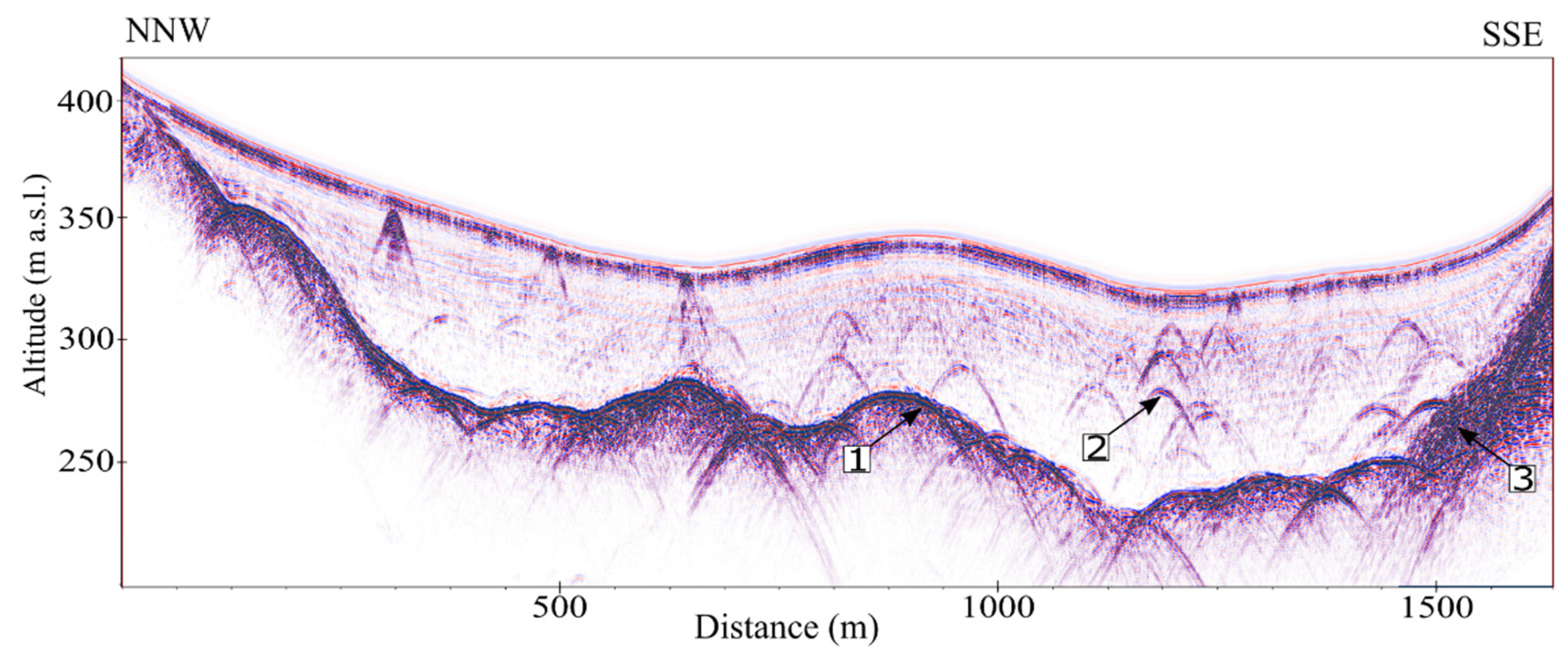
We identified many hyperbolic reflections across the glacier (Figure 4). We presume that the majority of them are linked to englacial conduits as has been noted in many studies [14,67,68,69]. Nonetheless, some could also be linked to crevasses or englacial debris bands or large boulders [70], especially close to glacier margins. We were able to use 75 hyperbolic reflections for the GPR signal propagation speed determination. It was calculated that the corresponding ε was equal to 3.34 ± 0.05 at the 95% confidence level (corresponding GPR signal propagation speed of 164.04 m ms−1).
In radargram that was obtained by recording CMP measurements, a clear reflection from glacier bed is evident (Figure 5a). It was possible to identify reflection from the glacier bed on all 99 recorded traces. Using obtained measurements, it was calculated that the corresponding ε was equal to 3.14 with the corresponding squared correlation coefficient 0.999 (Figure 5b) (corresponding GPR signal propagation speed of 169.18 m ms−1). Considering the arguments of [50], we assume that value of GPR signal propagation speed is determined with 2% error.
4.2. Ice Thickness, Surface and Subglacial Topography
The maximum measured ice thickness of Irenebreen reaches 145 m. The average ice thickness is 49 m. Calculated depth uncertainty near the glacier margin, where the ice depth is ~10 m is ±1.20 m, while at the highest part where ice thickness is ~145 m, it is ±3.13 m.
The ice volume equals to 143,956,421 m3 (0.14 km3) (Figure 6b). If for the volume calculations a value of ε = 3.34 is used (164.04 m ms−1), ice volume equals to 139,491,377 m3 and with ε = 3.2 (167.59 m ms−1) it equals to 142,158,464 m3. Thus, the highest difference in the ice volume, calculated form ice thickness models generated using different GPR propagation speeds, reached 3%.
The area with the greatest ice thickness is located in the south-eastern cirque of Irenebreen and coincides with the circular subglacial depression (Figure 6b,c). Exactly downstream from this depression, an elevated bedrock bump is found, which causes the locally extensional glacier stress regime. This is reflected also in the glacier surface, where the most crevassed area of Irenebreen is found (Figure 1c,e and Figure 6a). The more central part of the glacier surface comprises a shallow subglacial depression. Thus, the longitudinal profile of the surface of Irenebreen comprises areas of a prominent steepness (bumps) interrupted by areas of lesser steepness (depressions).
Altogether, the glacier bed decreases in the direction of the glacier terminus from 794 to 94 m a.s.l. Thus, the amplitude of the glacier bed altitude reaches 700 m. The irregular subglacial topography seems to be well inherited in the glacier surface and it is reflected in the glacier stress pattern as well. The elevated and lowered parts of glacier surface coincide very well with the pattern of subglacial topography and ice thickness (Figure 6a–c and Figure 7a).
The glacier surface is cut by several supraglacial stream systems (Figure 1d and Figure 6a). Several of the supraglacial streams begin at a close distance for the glacier terminus but the two largest incised stream systems develop at higher altitude (<400 m a.s.l.). The northern largest supraglacial stream seems to collect meltwater from all northern cirque of the glacier. These streams, in the same place, are observed for many years [31,32]. Nearby the glacier terminus, highly meandering streams are visible due to the lower surface inclination (Figure 1d). The mean slope angle of the glacier is 13 degrees. The steepest part of the glacier excluding the steep slopes of glacier cirque, is the southern part close to the highest mountain ridge. These slopes have mainly north-western exposition, thus receiving lesser amount of solar radiation (Figure 7a,b). The southern marginal part of the glacier is considerably steeper than the northern one.
4.3. Extent and Geometry of Temperate Ice
By examining the obtained radargrams, it was evident that in the most part of the glacier almost none or very weak internal reflections occur. Only in the upper part of the glacier, as well as at two areas close to the glacier southern margin, intense internal scattering of the GPR signal can be seen (Figure 4, Figure 8c and Figure 9b).
The area of the intense scattering zone that is located in the upper part of the glacier (accumulation area) occupies 0.46 km2. According to numerous studies where direct temperature measurements in boreholes were correlated with GPR survey results in attempts to explain such intense scattering [5,6,14,28,65,68,71,72], we interpret it as indication of temperate ice. The volume of temperate ice in Irenebreen equals to 16,950,676 m3 (0.017 km3). Considering the extent of the Irenebreen glacier (2.90 km2) and volume (0.14 km3), the horizontal distribution of the temperate ice is 16% but the volume reaches 12% of the total glacier volume. The average thickness of the temperate ice is 36.5 m, while its maximum thickness reaches 89 m in local subglacial deepening (Figure 8a,b), which also coincides with the thickest ice region (Figure 6b). Thus, the thickness of the temperate ice correlates very well with the thickness of all the glacier ice.
Considering that the average thickness of ice, solely in the area where the temperate ice is distributed, equals 73 m, the average temperate ice thickness is exactly two time less. Thus, the temperate ice layer on average occupies half of ice thickness in its distribution area, which is also well visible in Figure 8d. The maximal measured depth of the upper surface of the temperate ice layer (from the glacier surface) is 76 m, but the mean depth of the surface of the temperate ice layer is 43 m. The range of the altitude of the temperate ice surface stretches from 364 to 649 m a.s.l., although it could stretch slightly higher because the highest GPR profile begins some 200 m from the uppermost glacier margin, where the altitude of the glacier surface reach ~750 m a.s.l.
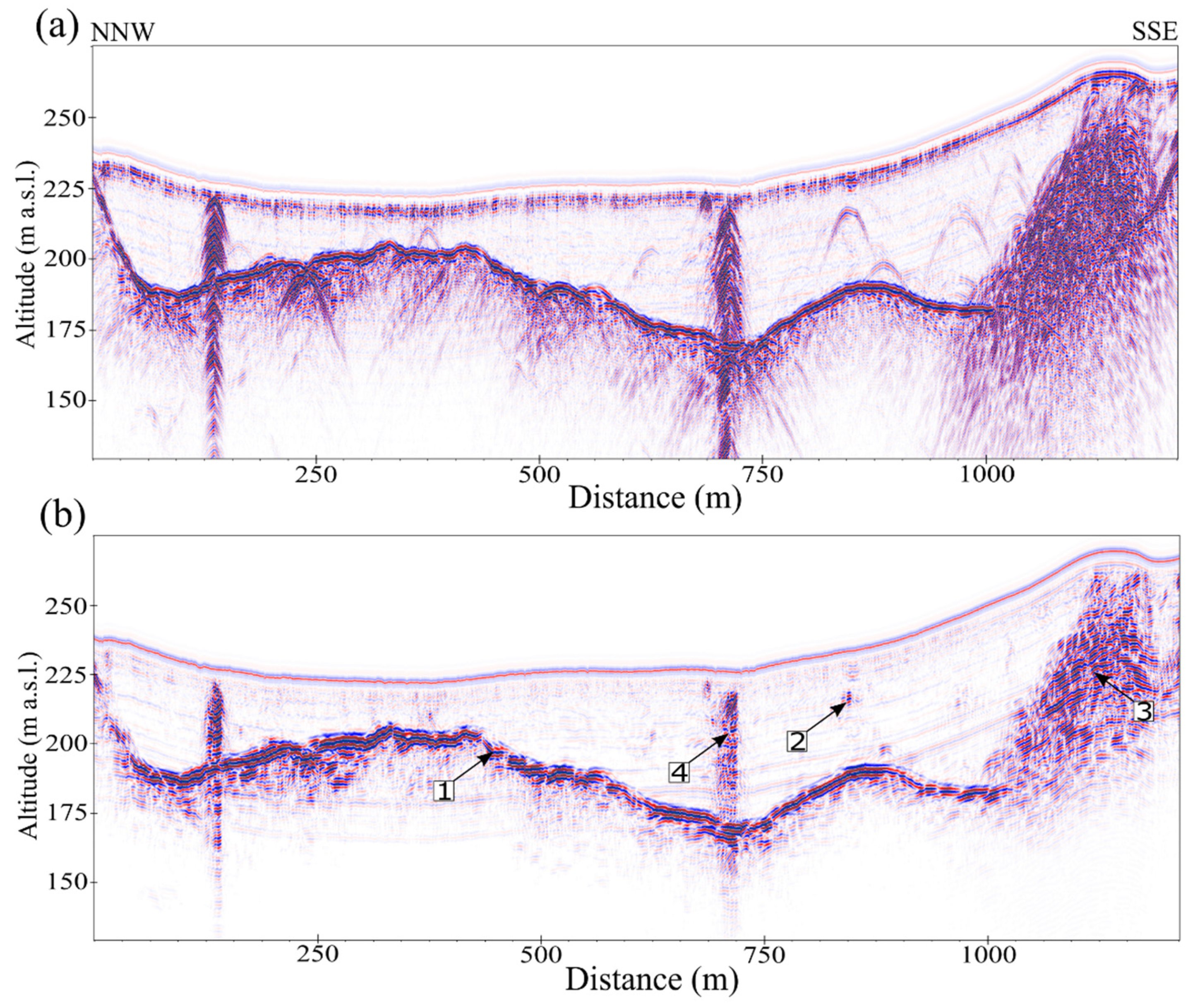
Two small intense scattering areas, which are located in the southern part of the glacier, occupy only 0.11 km2 (Figure 4 and Figure 9b). Contrary to the upper reaches of the glacier, these zones of intense scattering begin almost at the glacier surface. Several, rather distinct hyperbolas can be clearly seen in unmigrated data in the upper part of those zones (Figure 4 and Figure 9a). Those observations as well as observations from the field suggest that in the upper part of those zones, deep crevasses have formed in the relation to steep bedrock slopes.
5. Discussion
5.1. UAV Survey
In this study, we used UAV and GPR data integration to construct the glacier geometry. Using DJI Phantom 4 UAV with RTK system and placing 25 GCPs, we were able to map a larger area just in one day. The only downside of this method is the availability of a reference base station throughout the survey to provide PPK corrections for UAV trajectories. In our previous study of the adjacent glacier (Waldemarbreen) in 2019, we a used DJI Phantom 4 Pro V2.0 setup with many (~50) GCPs [57]. This survey setup required more than twice as long a time, because of GCP placement. Thus, the RTK system allows substantially shorten the time necessary for field-campaign, but the question of the sufficient number of GCPs and following RMSE remains disputable.
Peppa M.V. et al. in their study [62] mention that overall RMSE of their survey was less than 1 × GSD. The flight altitudes of their surveys were around 50–70 m, therefore for Phantom 4 RTK GSD at these altitudes was ~16 mm. The authors conclude that a combination of nadir and oblique images, as well as image acquisition on different heights can improve the overall precision of the survey.
Sanz-Ablanedo et al. concluded [73] that a total RMSE of the survey can be ~2 times GSD if more than 2 GCPs are used for each 100 images in the survey. With a bigger GCP count, the overall RMSE will decrease, but not indefinitely. In our survey, the average GSD was 4.29 cm/px according to Agisoft Metashape report. We acquired 4979 images and placed 25 GCPs (22 were used in the post-production), which equals to ~2 GCPs per 100 images. The average RMSE of check points was 14.8 cm, which is more than 3 times higher value than GSD. From our observations with greater flying altitudes, it gets more difficult to find the exact position of the center of GCP on the obtained images. We used GCP markers that are 50 cm × 50 cm in size. With the calculated GSD, they are ~11 pixels wide on the source images. The center of the GCP is less than a pixel. Average RMSE of the check points in pixels was 0.422 pix. In contrast, RMSE of image coordinates from the RTK module was 32 cm. Since the image acquisition is instantaneous, RMSE from such measurements is 0. The provided RMSE in Agisoft Metashape report is calculated based on GCPs and self-calibrated bundle adjustment. For higher accuracy, lower flight altitudes are required. In harsh polar conditions, it means that such a survey will consume more battery power and will take several days to complete. The use of multiple RTK UAV systems may be considered for faster performance.
It is obvious that with the development of new methods for georeferencing of the UAV imagery, new error estimation methods are needed. These estimation methods must include ground reference and flight reference combined in a single metric that will describe the accuracy of the survey. For now, there are many solutions for GNSS signal corrections, including RTKlib and Emlid Studio. These programs are suitable for Stop-and-Go surveys as well as trajectory corrections. However, they lack the possibility to calculate image coordinates for DJI Phantom RTK UAV system. The main problem is camera sensor position synchronization with the UAV position. We used Aerotas XLS workbook [56] that appeared to be a useful solution for this type of task. The terrain-following function of DJI Phantom RTK system allowed us to obtain constant GSD throughout the survey. Additional GCP control proved the high accuracy of the model. Using UAV, it was possible to create a high-resolution glacier surface model that was used to perform smooth topographic correction for the obtained GPR profiles.
5.2. GPR Data Processing and Interpretation
Typically for cold ice GPR signal propagation, a speed value of ~168 m ms−1 (ε = 3.2) is used [25,52,65,66]. This value is usually obtained in a laboratory by undertaking measurements in pure crystalline ice [74] (pp. 198–246), as well as in samples of glacier ice [75,76]; also, this value is obtained in most cases of direct measurements in the field, where glaciers consist of cold ice [24] (pp. 32–48).
In this study, we used two methods to calculate GPR signal propagation speed. With the CMP method, we obtained value of 169.18 m ms−1 (ε = 3.14). This value corresponds well with typical values that are reported for cold ice. It is a little bit higher but still in the uncertainty range of 2% that we adopted from [55]. Taking into account the previously mentioned study, we adopted with the CMP method determined GPR signal propagation speed value for further calculations.
As a second method we used internal hyperbolic reflections. This method is comparatively easy to use as it does not require additional measurements in the field, contrary to the CMP method. As a result, it is used quite often [11,51,52]. We obtained a value of 164.04 m ms−1 (ε = 3.34) that fits in the interval of values that are reported for temperate glaciers 167.59–139.78 m ms−1 (ε = 3.2–4.6) [7,52,77,78,79]. Nonetheless, we were able to sample hyperbolas only in regions where cold ice is present. Furthermore, we would expect a value that is closer to 167.59 m ms−1 (ε = 3.2). It is rather hard to explain such difference because value of 167.59 m ms−1 (ε = 3.2) does not fit in our determined uncertainty range (3.34 ± 0.05). Usually, such deviations are addressed to out of plain reflectors or linear features (in this case englacial conduits) that are crossed not perpendicularly [80] (pp. 625–649). Although the aforementioned issues would increase the obtained GPR signal propagation speed value, not decrease it. In our case, we explain this issue with ambiguities during hyperbola identification. In many cases, there were several overlapping hyperbolas, and the reflections themselves were weak. We calculated glacier volume using ε = 3.14 (169.18 m ms−1) and ε = 3.34 (164.04 m ms−1). Obtained volume difference is 3%. Our results show that whenever possible CMP or direct correlation of GPR reflections to borehole data are advisable and hyperbolic reflections should be used as a last option for GPR signal propagation speed determination.
During the calculations, we did not take into account the snow cover thickness. Nonetheless, almost all of the glacier was snow-free. There were some small areas in both cirques as well as along Southern margin of the glacier where snow was present, but the snow cover was very thin. Also, we were not able to reliably identify it on the recorded GPR profiles. Considering the previously mentioned facts, ice volume is very slightly overestimated. As snow cover was thin and only present at some places, we assume that corresponding volume error is below 1%.
In this study, we were unable to measure GPR signal propagation speed in temperate ice. Subsequently, we calculated the volume of the glacier and the volume of temperate ice using single value of GPR signal propagation speed (corresponding ε = 3.14 (169.18 m ms−1)). This results in overestimation of calculated volume of temperate ice and subsequently, the whole glacier. Temperate ice values as high as ε = 4.6 (139.78 m ms−1) are reported [52] and we do not exclude the possibility that this value could be even higher. If value of ε = 4.6 (139.78 m ms−1) were used instead of 3.14 (169.18 m ms−1), average thickness of temperate ice would decrease from 36.5 m to 30.2 m while maximum thickness would decrease from 89 m to 73.6 m. Accordingly also the volume of temperate ice would decrease to 14,004,666 m3. This volumetric difference equals to 17.4%. and can be considered as substantial, suggesting the importance of the GPR propagation speed in temperate ice, which is still not a sufficiently addressed issue in glaciological studies. In this study, we used single GPR signal propagation speed value for the whole glacier and did not use different values for temperate ice, as we were not able to measure it. We also abstained from using the GPR signal propagation speed value for temperate ice that was obtained in similar studies. We did this because GPR signal propagation speed can vary greatly in temperate ice, if water content in the ice changes [52]. It leads to a wide range of possible values (ε = 3.5–4.6 (160.25–139.78 m ms−1) [6]), and it is ambiguous to choose a value that would be appropriate for this particular glacier. We argue that, if the detailed geometry of glacier must be reconstructed, it is necessary to obtain direct measurements for GPR signal propagation speed value in temperate ice. If it is not possible to use englacial hyperbolic reflections or CMP measurements, direct correlation of GPR data and boreholes must be used. Furthermore, a combination of GPR and reflection seismic data could be used if it is not possible to drill boreholes. GPR propagation speed in cold ice could be determined with hyperbolic reflections or CMP. In areas where temperate ice is present, seismic reflection method could be used to determine the thickness of the glacier, and, in turn, this data could be used to calculate GPR propagation speed in temperate ice.
5.3. Internal Structure of Irenebreen
During the survey, we discovered a wide area of the intense GPR signal scattering in the upper part of the glacier (Figure 8). Such observations are common across Svalbard valley glaciers (e.g., [5,6,28]) and are usually interpreted as indicator of temperate ice. Our observations reveal that Irenebreen, similar to its neighbouring Waldemarbreen [14] is indeed a polythermal glacier with cold ice and a basal temperate ice layer, the volume of which reaches 10% to 12% of all glacier volume depending on the used GPR signal propagation speed in the temperate ice. The existence of possible basal temperate ice has been suggested by Sobota [31] due to the presence of icings in the forefield of Irenebreen. However, it should be noted that icings were missing during the field campaign in August 2021 (Figure 1b), although they have been observed at least since 1938 and every year from 2002 to 2020 [31,35]. This alarming sign of melting is closely related to the warming trend observed in all Svalbard [81] and in the Kaffiøyra region particularly, where summer air temperature has increased by 1.2 °C from 1975 to 2017 [37]. Thus, it should be considered that icings in front of glaciers in the Kaffiøyra region may be missing during summers, thus their existence or absence cannot be always used as a proof for the polythermal glacier regime. As already pointed out by several studies [68,69,82], the existence of icings is not always a proof for polythermal glacier ice as well.
The presence of temperate ice in Irenebreen is not surprising, as such thermal structures have been reported for similar valley glaciers in Svalbard [6,83] including the neighbouring Waldemarbreen [14]. However, it has distinct peculiarities. The presence of temperate ice is found only in the southern cirque. The northern glacier cirque contains only cold ice. This could be explained by the differences in altitude and ice thickness. The southern cirque extends at least 200 m higher reaching 700 m. The differences in ice thickness are essential, because the maximum ice thickness in the northern cirque reach only 83 m, while in the southern cirque it is 145 m (measured), being almost two times larger. Similar ice thickness is recorded in the neighbouring Waldemarbreen [14], which also contains temperate ice of similar thickness in its cirque. A simplified explanation of the lack of temperate ice in the northern cirque of Irenebreen could be a missing threshold ice thickness of 80–100 m, which is required for temperate ice to persist [84]. The other factors are high ELA and lack of crevasses, which could lead to the freezing of meltwater and related release of latent heat. In contrast, all supraglacial meltwater in the northern cirque seems to be drained by the extensive supraglacial streams (Figure 6a and Figure 7a). The area of temperate ice in the southern cirque coincides well not only with the area of the thickest ice (Figure 6b), but also with the most crevassed part of the glacier (Figure 1c,e and Figure 6a,b) that on the other hand is related to subglacial topography. Thus, the formation of temperate ice could be ongoing nowadays due to the refreezing of rain and meltwater that is known as cryo-hydrologic warming effect [85]. Nevertheless, such a thick layer of temperate ice at least partially could be considered as a relict form the Little Ice Age (LIA) because of a larger extent (by at least 35–36%) and associated thickness and velocity of the glacier.
Additionally, it can be a proof that due to climate warming (mainly a large ablation during summer and enhanced surface runoff due to melting snow, firn and ice, limited water percolation and refreezing in firn) Irenebreen may evolve into a cold glacier type, as other Svalbard glaciers (e.g., [14,31]).
We also observed the intense scattering, not only in the upper part of the glacier, but also in two small areas that are located along the southern lateral margin of the glacier (Figure 4 and Figure 9b). These zones of intense scattering begin almost at the glacier surface and in the upper part of them several hyperbolas can be clearly seen (Figure 4 and Figure 9a). We link these hyperbolas to deep crevasses. According to [42], who observed similar phenomena in an Alpine glacier, we suggest that intense water percolation occurs in these places. Furthermore, the geometry of these zones and characteristics of GPR signal suggest the occurrence of local areas of temperate ice, which are formed due to latent heat release from percolated meltwater in deep-seated crevasses. The survival of these local temperate ice zones most likely is related to the insulating effect of firn and snow cover that is mainly present all year round in this northern exposition slope. This finding emphasizes the possible formation of localised temperate ice zones in polythermal glaciers due to the coincidence of several specific factors (slope steepness and exposition, shadow, snow cover, crevasses, meltwater refreezing).
6. Conclusions
Our study demonstrates that an integrated approach of UAV and GPR survey is probably the most effective solution today for the high-resolution reconstruction of small glacier geometry. Such a simultaneous survey allows for obtaining DEM and ice thickness and internal structure data, which can be used for the integrated representation of the glacier surface characteristics, including slope and aspect, subglacial topography, thermal structure, and ice volume.
The maximum ice thickness of Irenebreen reaches at least 145 m, but the average thickness is 49 m. The ice volume is 0.14 km3, and 12% of it consists of temperate ice with an average thickness of 36.5 m (two time less than the average ice thickness in this part of the glacier) and the maximum thickness of 89 m. New GPR data reveal that Irenebreen is a polythermal glacier with basal temperate ice layer located mainly in the higher (southern) glacier cirque. Two small areas of temperate ice are found also in the ablation area along the southern margin of the glacier and are related to the intensive water penetration and re-freezing, which warms the adjacent ice.
Our results suggest that whenever possible CMP or direct correlation of GPR reflections to borehole data are advisable and hyperbolic reflections should be used as a last option for GPR signal propagation speed determination. Uncertainty in the value of GPR signal propagation speed in temperate ice can seriously impact calculations in temperate ice volume. We argue that, if a detailed geometry of glacier must be reconstructed, it is necessary to obtain direct measurements for GPR signal propagation speed value in temperate ice. If it is not possible to use englacial hyperbolic reflections or CMP measurements, direct correlation of GPR data and boreholes must be used.
Author Contributions
Conceptualization, J.K. and K.L.; methodology, J.K., K.L. and J.J.; software, J.J.; investigation, J.K., K.L., P.D. and J.J.; writing—original draft preparation, J.K., K.L., I.S. and J.J.; writing—review and editing, J.K., K.L., J.J.; visualization, K.L., P.D. and J.J. All authors have read and agreed to the published version of the manuscript.
Funding
This research was funded by the Latvian Council of Science, project “Thermal structure, drainage system and surface changes of Kaffiøyra Region glaciers, north-western Svalbard”, project No. lzp-2020/2-0279 and by the University of Latvia grant No. AAp2016/B041//Zd2016/AZ03 project “Climate change and sustainable use of natural resources”. It was carried out as part of the ‘Changes of northwestern Spitsbergen glaciers as the indicator of contemporary transformations occurring in the cryosphere’ (2017/25/B/ST10/00540) project funded by the National Science Centre, Poland.
Data Availability Statement
The data presented in this study are available on request from the corresponding author.
Acknowledgments
The authors thank all members of the Nicolaus Copernicus University expedition to Svalbard in 2021.
Conflicts of Interest
The authors declare no conflict of interest. The funders had no role in the design of the study; in the collection, analyses, or interpretation of data; in the writing of the manuscript, or in the decision to publish the results.
References
- Schuler, T.V.; Kohler, J.; Elagina, N.; Hagen, J.O.M.; Hodson, A.J.; Jania, J.A.; Kääb, A.M.; Luks, B.; Małecki, J.; Moholdt, G.; et al. Reconciling Svalbard Glacier Mass Balance. Front. Earth Sci. 2020, 8, 156. [Google Scholar] [CrossRef]
- Bahr, D.B.; Radić, V. Significant contribution to total mass from very small glaciers. Cryosphere 2012, 6, 763–770. [Google Scholar] [CrossRef] [Green Version]
- Colucci, R.R.; Forte, E.; Boccali, C.; Dossi, M.; Lanza, L.; Pipan, M.; Guglielmin, M. Evaluation of Internal Structure, Volume and Mass of Glacial Bodies by Integrated LiDAR and Ground Penetrating Radar Surveys: The Case Study of Canin Eastern Glacieret (Julian Alps, Italy). Surv. Geophys. 2015, 36, 231–252. [Google Scholar] [CrossRef]
- Navarro, F.J.; Martín-Espanol, A.; Lapazaran, J.J.; Grabiec, M.; Otero, J.; Vasilenko, E.V.; Puczko, D. Ice volume estimates from ground-penetrating radar surveys, wedel Jarlsberg land glaciers, Svalbard. Arc. Antarct. Alp. Res. 2014, 46, 394–406. [Google Scholar] [CrossRef] [Green Version]
- Björnsson, H.; Gjessing, Y.; Hamran, S.E.; Hagen, J.O.; LiestøL, O.; Pálsson, F.; Erlingsson, B. The thermal regime of sub-polar glaciers mapped by multi-frequency radio-echo sounding. J. Glaciol. 1996, 42, 23–32. [Google Scholar] [CrossRef] [Green Version]
- Sevestre, H.; Benn, D.I.; Hulton, N.R.; Bælum, K. Thermal structure of Svalbard glaciers and implications for thermal switch models of glacier surging. J. Geophys. Res. Earth Surf. 2015, 120, 2220–2236. [Google Scholar] [CrossRef] [Green Version]
- Martín-Español, A.; Vasilenko, E.V.; Navarro, F.J.; Otero, J.; Lapazaran, J.J.; Lavrentiev, I.; Macheret, Y.Y.; Machío, F. Radio-echo sounding and ice volume estimates of western Nordenskiöld Land glaciers, Svalbard. Ann. Glaciol. 2013, 54, 211–217. [Google Scholar] [CrossRef]
- Andreassen, L.M.; Moholdt, G.; Kääb, A.; Messerli, A.; Nagy, T.; Winsvold, S.H. Data. In Monitoring Glaciers in Mainland Norway and Svalbard Using Sentinel; Andreassen, L.M., Ed.; Norwegian Water Resources and Energy Directorate (NVE): Oslo, Norway, 2021; pp. 14–27. [Google Scholar]
- Fischer, M.; Huss, M.; Hoelzle, M. Surface elevation and mass changes of all Swiss glaciers 1980–2010. Cryosphere 2015, 9, 525–540. [Google Scholar] [CrossRef] [Green Version]
- Paul, F.; Bolch, T.; Kääb, A.; Nagler, T.; Nuth, C.; Scharrer, K.; Shepherd, A.; Strozzi, T.; Ticconi, F.; Bhambri, R.; et al. The glaciers climate change initiative: Methods for creating glacier area, elevation change and velocity products. Remote Sens. Environ. 2015, 162, 408–426. [Google Scholar] [CrossRef] [Green Version]
- Lamsters, K.; Karušs, J.; Rečs, A.; Bērziņš, D. Detailed subglacial topography and drumlins at the marginal zone of Múlajökull outlet glacier, central Iceland: Evidence from low frequency GPR data. Polar Sci. 2016, 10, 470–475. [Google Scholar] [CrossRef]
- Kodde, M.P.; Pfeifer, N.; Gorte, B.G.H.; Geistd, T.; Höfle, B. Automatic glacier surface analysis from airborne laser scanning. Int. Arch. Photogramm. Remote Sens. 2007, 36, 221–226. [Google Scholar]
- Knoll, C.; Kerschner, H. A glacier inventory for South Tyrol, Italy, based on airborne laser scanner data. Ann. Glaciol. 2009, 53, 46–52. [Google Scholar] [CrossRef] [Green Version]
- Karušs, J.; Lamsters, K.; Sobota, I.; Ješkins, J.; Džeriņš, P.; Hodson, A. Drainage system and thermal structure of a High Arctic polythermal glacier: Waldemarbreen, western Svalbard. J. Glaciol. 2021, 1–14. [Google Scholar] [CrossRef]
- Lamsters, K.; Karušs, J.; Krievāns, M.; Ješkins, J. The thermal structure, subglacial topography and surface structures of the NE outlet of Eyjabakkajökull, east Iceland. Polar Sci. 2020, 100566. [Google Scholar] [CrossRef]
- Lamsters, K.; Karušs, J.; Krievāns, M.; Ješkins, J. High-resolution orthophoto map and digital surface models of the largest Argentine Islands (the Antarctic) from unmanned aerial vehicle photogrammetry. J. Maps 2020, 16, 335–347. [Google Scholar] [CrossRef]
- Lamsters, K.; Karušs, J.; Krievāns, M.; Ješkins, J. High-Resolution Surface and Bed Topography Mapping of Russell Glacier (SW Greenland) Using UAV and GPR. ISPRS Ann. Photogramm. Remote Sens. Spat. Inf. Sci. 2020, 2, 757–763. [Google Scholar] [CrossRef]
- Śledź, S.; Ewertowski, M.; Piekarczyk, J. Applications of unmanned aerial vehicle (UAV) surveys and Structure from Motion photogrammetry in glacial and periglacial geomorphology. Geomorphology 2021, 378, 107620. [Google Scholar] [CrossRef]
- Ewertowski, M.W.; Tomczyk, A.M.; Evans, D.J.A.; Roberts, D.H.; Ewertowski, W. Operational Framework for Rapid, Very-high Resolution Mapping of Glacial Geomorphology Using Low-cost Unmanned Aerial Vehicles and Structure-from-Motion Approach. Remote Sens. 2019, 11, 65. [Google Scholar] [CrossRef] [Green Version]
- Bash, E.A.; Moorman, B.J.; Gunther, A. Detecting Short-Term Surface Melt on an Arctic Glacier Using UAV Surveys. Remote Sens. 2018, 10, 1547. [Google Scholar] [CrossRef] [Green Version]
- Bhardwaj, A.; Sam, L.; Martín-Torres, F.J.; Kumar, R. UAVs as remote sensing platform in glaciology: Present applications and future prospects. Remote Sens. Environ. 2016, 175, 196–204. [Google Scholar] [CrossRef]
- Cao, B.; Guan, W.; Li, K.; Pan, B.; Sun, X. High-Resolution Monitoring of Glacier Mass Balance and Dynamics with Unmanned Aerial Vehicles on the Ningchan No. 1 Glacier in the Qilian Mountains, China. Remote Sens. 2021, 13, 2735. [Google Scholar] [CrossRef]
- Pellikka, P.; Rees, W.G. Remote Sensing of Glaciers. In Techniques for Topographic, Spatial and Thematic Mapping of Glaciers; Taylor & Francis Group: London, UK, 2009; p. 330. [Google Scholar]
- Bogorotsky, V.V.; Bentley, C.R.; Gudmandsen, P.E. Radioglaciology; D. Reidel Publishing Co.: Dordrecht, The Netherlands, 1985; pp. 32–48. [Google Scholar]
- Fischer, A.; Kuhn, M. Ground-penetrating radar measurements of 64 Austrian glaciers between 1995 and 2010. Ann. Glaciol. 2013, 54, 179–188. [Google Scholar] [CrossRef] [Green Version]
- Church, G.; Bauder, A.; Grab, M.; Rabenstein, L.; Singh, S.; Maurer, H. Detecting and characterising an englacial conduit network within a temperate Swiss glacier using active seismic, ground penetrating radar and borehole analysis. Ann. Glaciol. 2019, 60, 193–205. [Google Scholar] [CrossRef] [Green Version]
- Booth, A.; Mercer, A.; Clark, R.; Murray, T.; Jansson, P.; Axtell, C. A comparison of seismic and radar methods to establish the thickness and density of glacier snow cover. Ann. Glaciol. 2013, 54, 73–82. [Google Scholar] [CrossRef] [Green Version]
- Ødegård, R.S.; Hamran, S.E.; Bø, P.H.; Etzelmuller, B.; Vatne, G.; Sollid, J.L. Thermal regime of a valley glacier, Erikbreen, northern Spitsbergen. Polar Res. 1992, 11, 69–79. [Google Scholar] [CrossRef]
- Sobota, I. Physical geography of Kaffiøyra. In Atlas of Changes in the Glaciers of Kaffiøyra (Svalbard, the Arctic); Sobota, I., Ed.; Wydawnictwo Naukowe Uniwersytetu Mikołaja Kopernika: Toruń, Poland, 2021; pp. 51–65. [Google Scholar]
- Sobota, I. Glaciers of Svalbard. In Atlas of Changes in the Glaciers of Kaffiøyra (Svalbard, the Arctic); Sobota, I., Ed.; Wydawnictwo Naukowe Uniwersytetu Mikołaja Kopernika: Toruń, Poland, 2021; pp. 29–47. [Google Scholar]
- Sobota, I. Snow accumulation, melt, mass loss, and the near-surface ice temperature structure of Irenebreen, Svalbard. Polar Sci. 2011, 5, 327–336. [Google Scholar] [CrossRef] [Green Version]
- Wójcik, K.A.; Sobota, I. Spatial and temporal changes in ablation, distribution and evolution of glacial zones on Irenebreen, a small glacier of the High Arctic, Svalbard. Polar Sci. 2020, 23, 100503. [Google Scholar] [CrossRef]
- Sobota, I. Selected problems of snow accumulation on glaciers during long-term studies in north-western Spitsbergen, Svalbard. Geogr. Ann. Ser. A Phys. Geogr. 2017, 99, 177–192. [Google Scholar] [CrossRef]
- Sobota, I.; Weckwerth, P.; Grajewski, T. Rain-On-Snow (ROS) events and their relations to snowpack and ice layer changes on small glaciers in Svalbard, the high Arctic. J. Hydrol. 2020, 590, 125279. [Google Scholar] [CrossRef]
- Sobota, I.; Nowak, M.; Różański, K.M. Changes in glaciers of Kaffiøyra. In Atlas of Changes in the Glaciers of Kaffiøyra (Svalbard, the Arctic); Sobota, I., Ed.; Wydawnictwo Naukowe Uniwersytetu Mikołaja Kopernika: Toruń, Poland, 2021; pp. 109–185. [Google Scholar]
- Sobota, I.; Nowak, M.; Weckwerth, P. Long-term changes of glaciers in north-western Spitsbergen. Glob. Planet. Chang. 2016, 144, 182–197. [Google Scholar] [CrossRef]
- Kejna, M.; Sobota, I. Meteorological conditions on Kaffiøyra (NW Spitsbergen) in 2013–2017 and their connection with atmospheric circulation and sea ice extent. Pol. Polar Res. 2019, 40, 175–204. [Google Scholar]
- Kejna, M.; Sobota, I. Climate of Kaffiøyra. In Atlas of Changes in the Glaciers of Kaffiøyra (Svalbard, the Arctic); Sobota, I., Ed.; Wydawnictwo Naukowe Uniwersytetu Mikołaja Kopernika: Toruń, Poland, 2021; pp. 67–75. [Google Scholar]
- Galley, R.J.; Trachtenberg, M.; Langlois, A.; Barber, D.G.; Shafai, L. Observations of geophysical and dielectric properties and ground penetrating radar signatures for discrimination of snow, sea ice and freshwater ice thickness. Cold Reg. Sci. Technol. 2009, 57, 29–38. [Google Scholar] [CrossRef]
- Grab, M.; Mattea, E.; Bauder, A.; Huss, M.; Rabenstain, L.; Hodel, E.; Linsbauer, A.; Langhammer, L.; Schmid, L.; Church, G.; et al. Ice thickness distribution of all Swiss glaciers based on extended ground-penetrating radar data and glaciological modeling. J. Glaciol. 2021, 67, 1–19. [Google Scholar] [CrossRef]
- Egli, E.E.; Irving, J.; Lane, S.N. Characterization of subglacial marginal channels using 3-D analysis of high-density ground-penetrating radar data. J. Glaciol. 2021, 67, 1–14. [Google Scholar] [CrossRef]
- Forte, E.; Santin, I.; Ponti, S.; Colucci, R.R.; Gutgesell, P.; Guglielmin, M. New insights in glaciers characterization by differential diagnosis integrating GPR and remote sensing techniques: A case study for the Eastern Gran Zebrù glacier (Central Alps). Remote Sens. Environ. 2021, 267, 112715. [Google Scholar] [CrossRef]
- Jol, H. Ground Penetrating Radar Theory and Applications, 1st ed.; Elsevier Science: Amsterdam, The Netherlands, 2009. [Google Scholar]
- Leng, Z.; Al-Qadi, I.L. An innovative method for measuring pavement dielectric constant using the extended CMP method with two air-coupled GPR systems. NDTE Int. 2014, 66, 90–98. [Google Scholar] [CrossRef]
- Karušs, J.; Bērziņš, D. Ground-penetrating radar study of the Cenas tīrelis bog, Latvia: Linkage of reflections with peat moisture content. Bull. Geol. Soc. Finl. 2015, 87, 87–98. [Google Scholar] [CrossRef]
- Karušs, J.; Lamsters, K.; Poršņovs, D.; Zandersons, V.; Ješkins, J. 2021. Geophysical mapping of residual pollution at the remediated Inčukalns acid tar lagoon, Latvia. Est. J. Earth Sci. 2021, 70, 140–151. [Google Scholar]
- Murray, T.; Stuart, G.W.; Miller, P.J.; Woodward, J.; Smith, A.M.; Porter, P.R.; Jiskoot, H. Glacier surge propagation by thermal evolution at the bed. J. Geophys. Res. Solid Earth 2000, 105, 13491–13507. [Google Scholar] [CrossRef] [Green Version]
- Woodward, J.; Murray, T.; Clark, R.A.; Stuart, G.W. Glacier surge mechanisms inferred from ground-penetrating radar: Kongsvegen Svalbard. J. Glaciol. 2003, 49, 473–480. [Google Scholar] [CrossRef] [Green Version]
- Macheret, Y.Y.; Moskalevsky, M.Y. Velocity of radio waves in glaciers as an indicator of their hydrothermal state, structure and regime. J. Glaciol. 1993, 39, 373–384. [Google Scholar] [CrossRef] [Green Version]
- Barrett, B.E.; Murray, T.; Clark, R. Errors in radar CMP velocity estimates due to survey geometry, and their implication for ice water content estimation. JEEG 2007, 12, 101–111. [Google Scholar] [CrossRef]
- Moore, J.C.; Pälli, A.; Ludwig, F.; Blatter, H.; Jania, J.; Gadek, B.; Glowacki, P.; Mochnacki, D.; Isaksson, E. High-resolution hydrothermal structure of Hansbreen, Spitsbergen, mapped by ground-penetrating radar. J. Glaciol. 1999, 45, 524–532. [Google Scholar] [CrossRef] [Green Version]
- Bradford, J.H.; Harper, J.T. Wave field migration as a tool for estimating spatially continuous radar velocity and water content in glaciers. Geophys. Res. Lett. 2005, 32, L08502. [Google Scholar] [CrossRef] [Green Version]
- Karušs, J.; Lamsters, K.; Chernov, A.; Krievāns, M.; Ješkins, J. Subglacial topography and thickness of ice caps on the Argentine Islands. Antarct. Sci. 2019, 31, 332–344. [Google Scholar] [CrossRef]
- Navarro, F.; Eisen, O. Ground-penetrating radar in glaciological applications. In Remote Sensing of Glaciers. Techniques for Topographic, Spatial and Thematic Mapping of Glaciers; Pellikka, P., Rees, W.G., Eds.; Taylor & Francis Group: London, UK, 2009; pp. 195–231. [Google Scholar]
- Jacob, R.W.; Hermance, J.F. Assessing the precision of GPR velocity and vertical two-way travel time estimates. JEEG 2004, 9, 143–153. [Google Scholar] [CrossRef]
- Losè, L.T.; Chiabrando, F.; Tonolo, F.G. Are measured ground control points still required in UAV based large scale mapping? assessing the positional accuracy of an RTK multi-rotor platform. Int. Arch. Photogramm. Remote Sens. 2020, 43, 507–514. [Google Scholar] [CrossRef]
- Lamsters, K.; Karušs, J.; Krievāns, M.; Ješkins, J. Application of Unmanned Aerial Vehicles for Glacier Research in the Arctic and Antarctic. In Environment. Technologies. Resources, Proceedings of the 12th International Scientific and Practical Conference, Rezekne, Latvia, 20–22 June 2019; Rezekne Academy of Technologies: Rēzekne, Latvia, 2019; Volume 1, pp. 131–135. [Google Scholar]
- Forlani, G.; Dall’Asta, E.; Diotri, F.; Cella, U.M.D.; Roncella, R.; Santise, M. Quality assessment of DSMs produced from UAV flights georeferenced with on-board RTK positioning. Remote Sens. 2018, 10, 311. [Google Scholar] [CrossRef] [Green Version]
- Jiménez-Jiménez, S.I.; Ojeda-Bustamante, W.; Marcial-Pablo, M.; Enciso, J. Digital Terrain Models Generated with Low-Cost UAV Photogrammetry: Methodology and Accuracy. IJGI 2021, 10, 285. [Google Scholar] [CrossRef]
- Štroner, M.; Urban, R.; Reindl, T.; Seidl, J.; Brouček, J. Evaluation of the georeferencing accuracy of a photogrammetric model using a quadrocopter with onboard GNSS RTK. J. Sens. 2020, 20, 2318. [Google Scholar] [CrossRef] [Green Version]
- Taddia, Y.; Stecchi, F.; Pellegrinelli, A. Coastal mapping using DJI Phantom 4 RTK in post-processing kinematic mode. Drones 2020, 4, 9. [Google Scholar] [CrossRef] [Green Version]
- Peppa, M.V.; Hall, J.; Goodyear, J.; Mills, J.P. Photogrammetric assessment and comparison of DJI Phantom 4 Pro and Phantom 4 RTK small unmanned aircraft systems. In Proceedings of the International Archives of the Photogrammetry, Remote Sensing and Spatial Information Sciences, Enschede, The Netherlands, 10–14 June 2019; International Society for Photogrammetry and Remote Sensing: Stuttgart, Germany, 2019; Volume XLII-2/W13. [Google Scholar]
- Przybilla, H.-J.; Bäumker, M.; Luhmann, T.; Hastedt, H.; Eilers, M. Interaction between direct georeferencing, control point configuration and camera self-calibration for RTK-based UAV photogrammetry. In Proceedings of the International Archives of the Photogrammetry, Remote Sensing and Spatial Information Sciences, Nice, France, 31 August–2 September 2020; International Society for Photogrammetry and Remote Sensing: Stuttgart, Germany, 2020; Volume XLIII-B1-2020. [Google Scholar]
- James, M.R.; Chandler, J.H.; Eltner, A.; Fraser, C.; Miller, P.E.; Mills, J.P.; Noble, T.; Robson, S.; Lane, S.N. Guidelines on the use of structure-from-motion photogrammetry in geomorphic research. Earth Surf. Process. Landf. 2019, 44, 2081–2084. [Google Scholar] [CrossRef]
- Gusmeroli, A.; Murray, T.; Jansson, P.; Pettersson, R.; Aschwanden, A.; Booth, A.D. Vertical distribution of water within the polythermal Storglaciären, Sweden. J. Geophys. Res. Earth Surf. 2010, 115. [Google Scholar] [CrossRef]
- Farinotti, D.; King, E.C.; Albrecht, A.; Huss, M.; Gudmundsson, G.H. The bedrock topography of Starbuck Glacier, Antarctic Peninsula, as determined by radio-echo soundings and flow modeling. Ann. Glaciol. 2014, 55, 22–28. [Google Scholar] [CrossRef] [Green Version]
- Stuart, G.; Murray, T.; Gamble, N.; Hayes, K.; Hodson, A. Characterization of englacial channels by ground-penetrating radar: An example from austre Brggerbreen, Svalbard. J. Geophys. Res. Solid Earth 2003, 108, 2525. [Google Scholar] [CrossRef]
- Bælum, K.; Benn, D.I. Thermal structure and drainage system of a small valley glacier (Tellbreen, Svalbard), investigated by ground penetrating radar. Cryosphere 2011, 5, 139–149. [Google Scholar] [CrossRef] [Green Version]
- Temminghoff, M.; Benn, D.I.; Gulley, J.D.; Sevestre, H. Characterization of the englacial and subglacial drainage system in a high Arctic cold glacier by speleological mapping and ground-penetrating radar. Geogr. Ann. A 2019, 101, 98–117. [Google Scholar] [CrossRef]
- Thompson, S.S.; Cook, S.; Kulessa, B.; Winberry, J.P.; Fraser, A.D.; Galton-Fenzi, B.K. Comparing satellite and helicopter-based methods for observing crevasses, application in East Antarctica. Cold Reg. Sci. Technol. 2020, 178, 103128. [Google Scholar] [CrossRef]
- Pettersson, R.; Jansson, P.; Holmlund, P. Cold surface layer thinning on Storglaciären, Sweden, observed by repeated ground penetrating radar surveys. J. Geophys. Res. 2003, 108, 6004–6005. [Google Scholar] [CrossRef]
- Hodgkins, R.; Hagen, J.O.; Hamran, S.E. 20th century mass balance and thermal regime change at Scott Turnerbreen, Svalbard. Ann. Glaciol. 1999, 28, 216–220. [Google Scholar] [CrossRef] [Green Version]
- Sanz-Ablanedo, E.; Chandler, J.H.; Rodríguez-Pérez, J.R.; Ordóñez, C. Accuracy of Unmanned Aerial Vehicle (UAV) and SfM photogrammetry survey as a function of the number and location of ground control points used. Remote Sens. 2018, 10, 1606. [Google Scholar] [CrossRef] [Green Version]
- Fletcher, N.H. The Chemical Physics of Ice; Cambridge University Press: Cambridge, UK, 1970; pp. 198–246. [Google Scholar]
- West, J.; Rippin, D.M.; Murray, T.; Mader, H.; Hubbard, B.P. Dielectric Permittivity measurements on ice cores: Implications for interpretation of radar to yield glacial unfrozen water content. J. Environ. Eng. Sci. 2007, 12, 37–45. [Google Scholar] [CrossRef] [Green Version]
- Fitzgerald, W.J.; Paren, J.G. The dielectric properties of Antarctic ice. J. Glaciol. 1975, 15, 39–48. [Google Scholar] [CrossRef] [Green Version]
- Bradford, J.H.; Nichols, J.T.; Mikesell, T.D.; Harper, J.T. Continuous profiles of electromagnetic wave velocity and water content in glaciers: An example from Bench Glacier, Alaska, USA. Ann. Glaciol. 2009, 50, 1–9. [Google Scholar] [CrossRef] [Green Version]
- Bradford, J.H.; Nichols, J.; Harper, J.T.; Meierbachtol, T. Compressional and EM wave velocity anisotropy in a temperate glacier due to basal crevasses, and implications for water content estimation. Ann. Glaciol. 2013, 54, 168–178. [Google Scholar] [CrossRef] [Green Version]
- Blindow, N.; Suckro, S.K.; Rückamp, M.; Braun, M.; Schindler, M.; Breuer, B.; Saurer, H.; Simões, J.C.; Lange, M.A. Geometry and thermal regime of the King George Island ice cap, Antarctica, from GPR and GPS. Ann. Glaciol. 2010, 51, 103–109. [Google Scholar] [CrossRef] [Green Version]
- Daniels, D.J. Ground Penetrating Radar, 2nd ed.; The Institution of Electrical Engineers: London, UK, 2004; pp. 625–646. [Google Scholar]
- Nørdli, Ø.; Przybylak, R.; Ogilvie, A.E.J.; Isaksen, K. Long-term temperature trends and variability on Spitsbergen: The extended Svalbard Airport temperature series, 1898–2012. Polar Res. 2014, 33, 21–49. [Google Scholar] [CrossRef] [Green Version]
- Mallinson, L.; Swift, D.A.; Sole, A. Proglacial icings as indicators of glacier thermal regime: Ice thickness changes and icing occurrence in Svalbard. Geogr. Ann. A 2019, 101, 334–349. [Google Scholar] [CrossRef]
- Irvine-Fynn, T.D.L.; Hodson, A.J.; Moorman, B.J.; Vatne, G.; Hubbard, A.L. Polythermal glacier hydrology: A review. Rev. Geophys. 2011, 49, RG4002. [Google Scholar] [CrossRef] [Green Version]
- Murray, T.; Stuart, G.W.; Fry, M.; Gamble, N.H.; Crabtree, M.D. Englacial water distribution in a temperate glacier from surface and borehole radar velocity analysis. J. Glaciol. 2000, 46, 389–398. [Google Scholar] [CrossRef] [Green Version]
- Phillips, T.; Rajaram, H.; Steffen, K. Cryo-hydrologic warming: A potential mechanism for rapid thermal response of ice sheets. Geophys. Res. Lett. 2010, 37, L20503. [Google Scholar] [CrossRef]
Figure 1.
(a) Location of the study site in 2021; (b–f) Characteristics of the glacier surface in 2021. Black arrows in (c,e) show the main uplift in the glacier surface with the most prominent crevasses. Black arrows in (d) mark the main meandering supraglacial streams in the NW part of Irenebreen. Black arrows in (f) mark the outline of snow in the accumulation area in August that coincides well with the glacier area in shadow. A red circle shows a researcher to indicate a scale; (g) CMP measurements are being conducted. Note the cross-cutting pattern of crevasse traces and closed crevasses indicating compressional stress regime.

Figure 2.
Location of the GPR profile lines and common midpoint (CMP) measurement site.
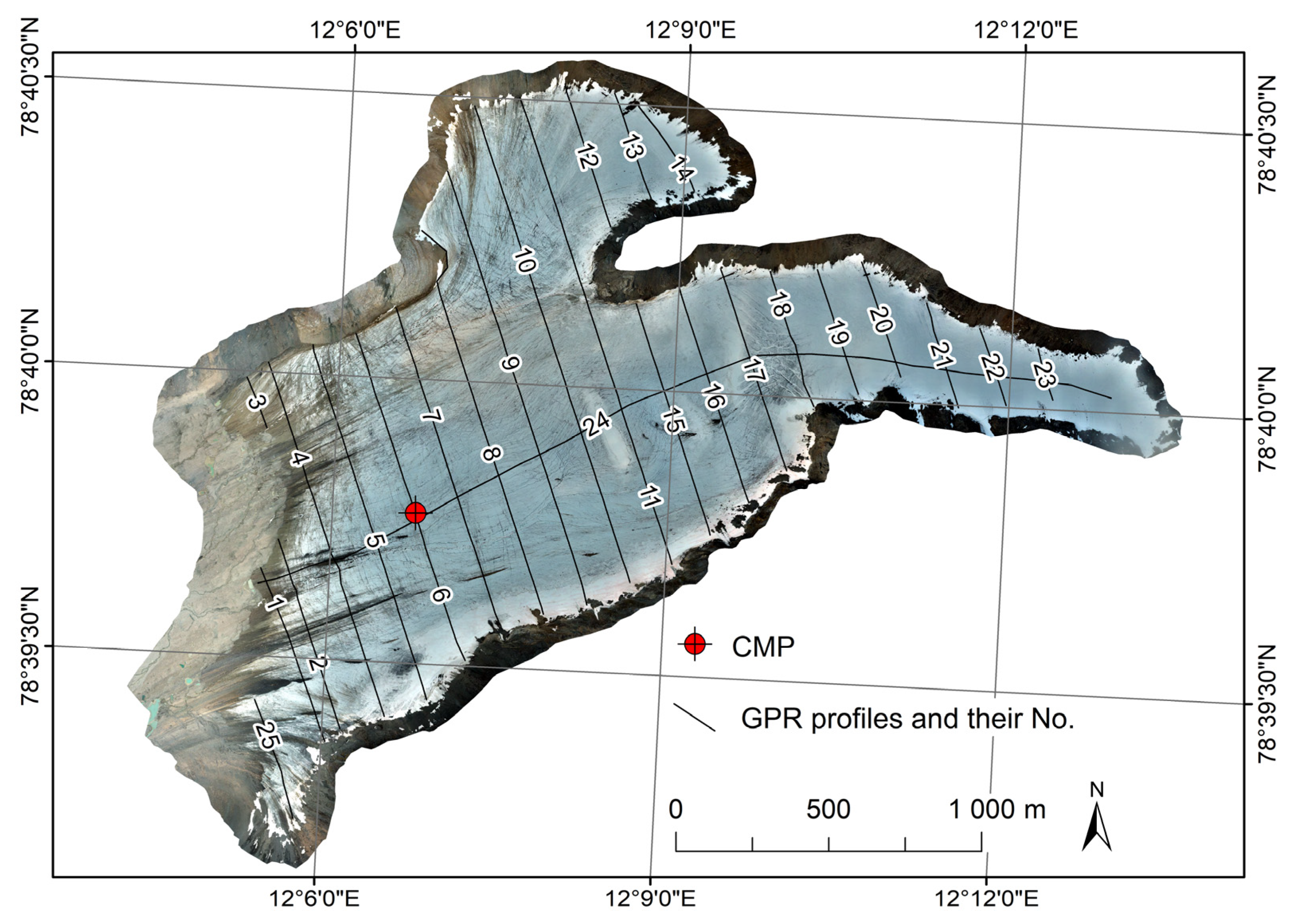
Figure 3.
UAV flight coverage areas on orthomosaic of Irenebreen in August 2021.
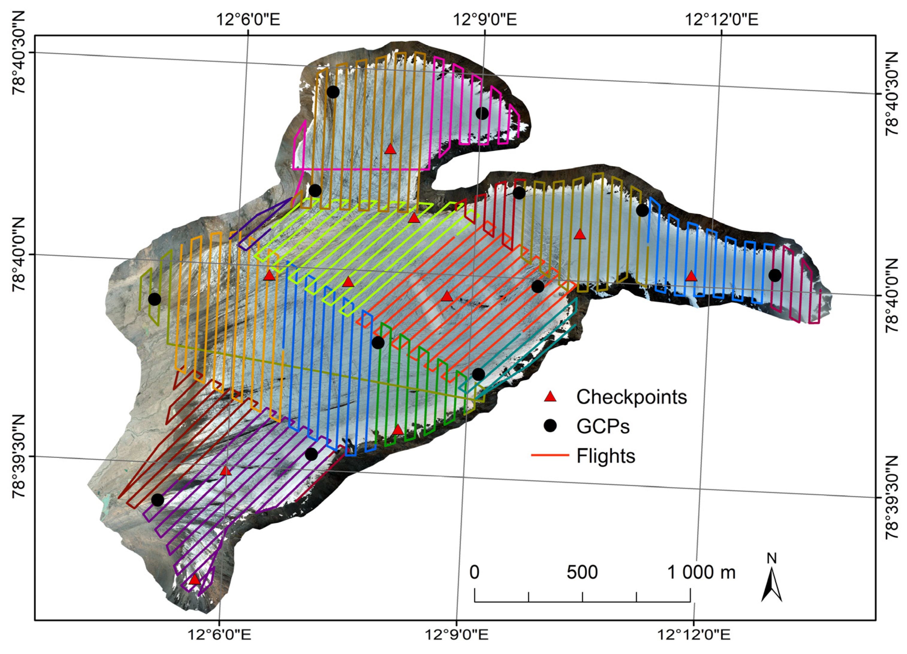
Figure 4.
GPR profile 10. Note that the profile is unmigrated for better identification of hyperbolic reflections. For the location of the profile see Figure 2. 1—glacier bed; 2—englacial hyperbolic reflection; 3—zone of intense scattering.
Figure 4.
GPR profile 10. Note that the profile is unmigrated for better identification of hyperbolic reflections. For the location of the profile see Figure 2. 1—glacier bed; 2—englacial hyperbolic reflection; 3—zone of intense scattering.

Figure 5.
(a) During CMP measurements obtained radargram; (b) Constructed t2x2 graph.
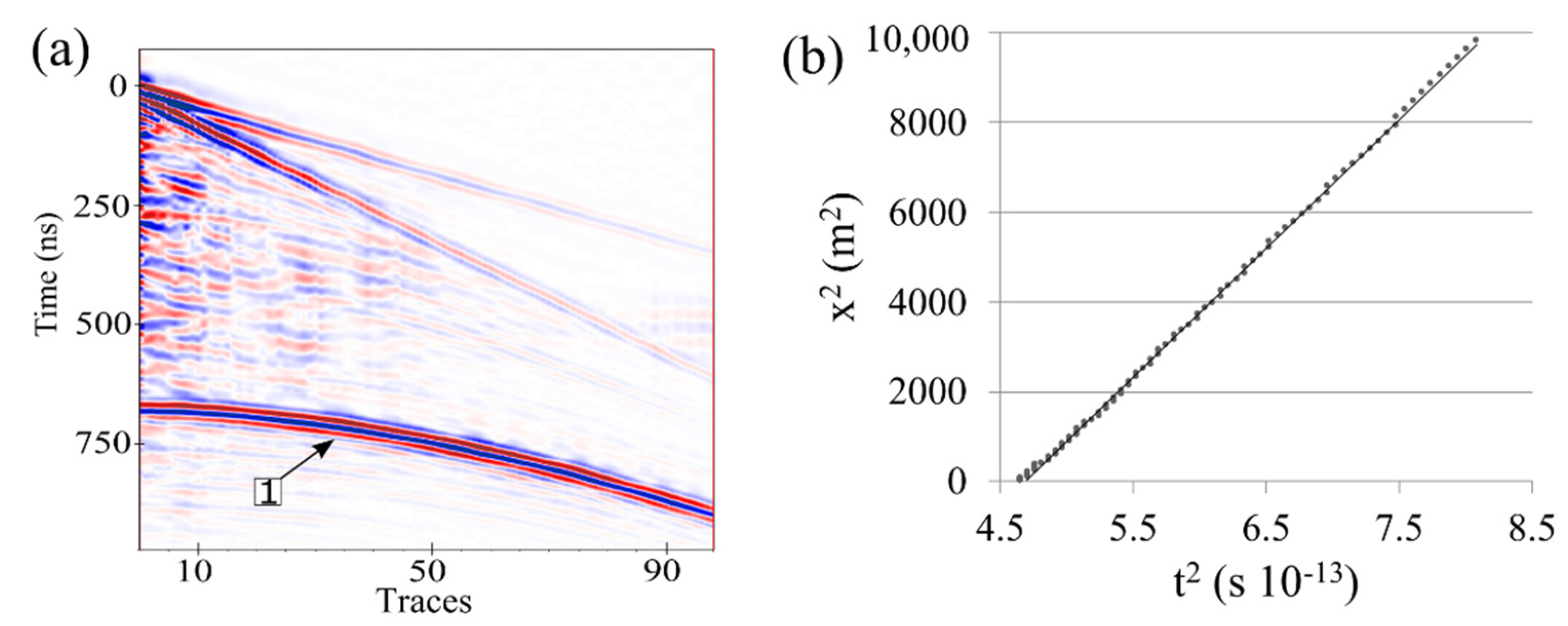
Figure 6.
Geometry of Irenebreen. (a) Hillshaded image of the glacier surface and adjacent mountain slopes; (b) Ice thickness and the horizontal distribution of the temperate ice; (c) Subglacial topography; (d) 3D model of the subglacial topography and the distribution of reflections from englacial hyperbolae.

Figure 7.
Surface characteristics of Irenebreen. (a) Slope; (b) aspect.
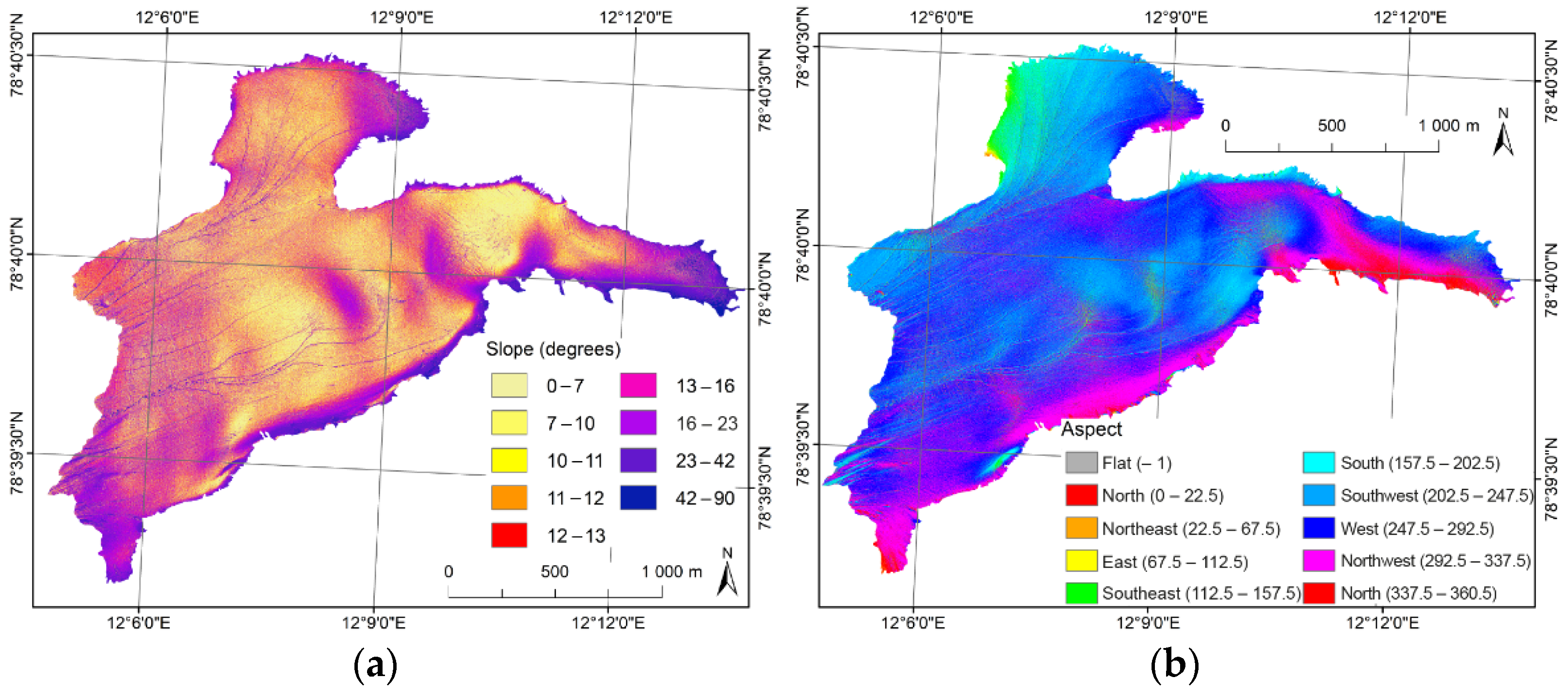
Figure 8.
(a,b) 2D and 3D representation of the temperate ice; (c) GPR profile No. 17. The location is shown by black line in (a); (d) Profile of glacier surface, temperate ice layer and bedrock surface. The location is shown by a red line in (a).
Figure 8.
(a,b) 2D and 3D representation of the temperate ice; (c) GPR profile No. 17. The location is shown by black line in (a); (d) Profile of glacier surface, temperate ice layer and bedrock surface. The location is shown by a red line in (a).
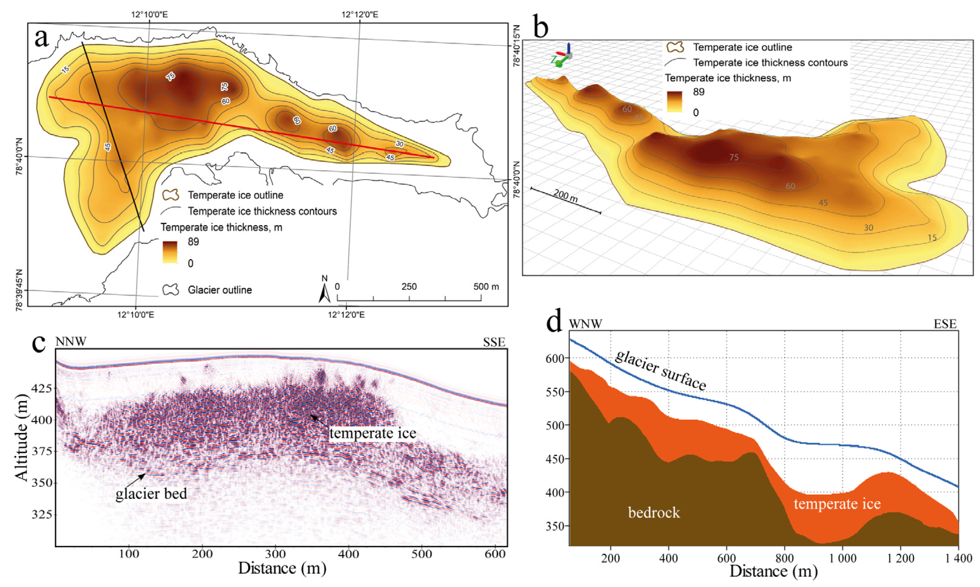
Figure 9.
Comparison of (a) unmigrated and (b) migrated GPR profile No. 5. For the location of profile see Figure 2. 1—glacier bed; 2—englacial hyperbolic reflection; 3—zone of intense scattering; 4—reflection from deeply incised supraglacial stream.
Figure 9.
Comparison of (a) unmigrated and (b) migrated GPR profile No. 5. For the location of profile see Figure 2. 1—glacier bed; 2—englacial hyperbolic reflection; 3—zone of intense scattering; 4—reflection from deeply incised supraglacial stream.
Publisher’s Note: MDPI stays neutral with regard to jurisdictional claims in published maps and institutional affiliations. |
© 2022 by the authors. Licensee MDPI, Basel, Switzerland. This article is an open access article distributed under the terms and conditions of the Creative Commons Attribution (CC BY) license (https://creativecommons.org/licenses/by/4.0/).
Share and Cite
MDPI and ACS Style
Karušs, J.; Lamsters, K.; Ješkins, J.; Sobota, I.; Džeriņš, P. UAV and GPR Data Integration in Glacier Geometry Reconstruction: A Case Study from Irenebreen, Svalbard. Remote Sens. 2022, 14, 456. https://doi.org/10.3390/rs14030456
AMA Style
Karušs J, Lamsters K, Ješkins J, Sobota I, Džeriņš P. UAV and GPR Data Integration in Glacier Geometry Reconstruction: A Case Study from Irenebreen, Svalbard. Remote Sensing. 2022; 14(3):456. https://doi.org/10.3390/rs14030456
Chicago/Turabian StyleKarušs, Jānis, Kristaps Lamsters, Jurijs Ješkins, Ireneusz Sobota, and Pēteris Džeriņš. 2022. "UAV and GPR Data Integration in Glacier Geometry Reconstruction: A Case Study from Irenebreen, Svalbard" Remote Sensing 14, no. 3: 456. https://doi.org/10.3390/rs14030456
Note that from the first issue of 2016, this journal uses article numbers instead of page numbers. See further details here.