Full-Waveform Inversion of Time-Lapse Crosshole GPR Data Using Markov Chain Monte Carlo Method

Abstract

Crosshole ground-penetrating radar (GPR) is an important tool for a wide range of geoscientific and engineering investigations, and the Markov chain Monte Carlo (MCMC) method is a heuristic global optimization method that can be used to solve the inversion problem. In this paper, we use time-lapse GPR full-waveform data to invert the dielectric permittivity. An inversion based on the MCMC method does not rely on an accurate initial model and can introduce any complex prior information. Time-lapse ground-penetrating radar has great potential to monitor the properties of a subsurface. For the time-lapse inversion, we used the double difference method to invert the time-lapse target area accurately and full-waveform data. We propose a local sampling strategy taking advantage of the a priori information in the Monte Carlo method, which can sample only the target area with a sequential Gibbs sampler. This method reduces the calculation and improves the inversion accuracy of the target area. We have provided inversion results of the synthetic time-lapse waveform data that show that the proposed method significantly improves accuracy in the target area.

1. Introduction

Crosshole ground-penetrating radar is widely used in geoscientific and engineering investigations (e.g., identify cracks, analysis moisture) [1,2]. It is a popular tool for mapping subsurface electrical properties, especially electrical conductivity and dielectric permittivity, which are closely related to the underground characteristics of environments (e.g., water content) [3,4,5,6]. It has also shown great potential for mapping and monitoring time-lapse changes, which improves our understanding of dynamic processes [7,8,9]. This technique uses transmitting radar antennas to generate high-frequency electromagnetic energy in a borehole to acquire crosshole radar data.

To invert GPR data, both deterministic inversion algorithms and probabilistic inversion methods have been proposed [10,11,12,13,14,15]. Most deterministic inversion methods depend on an accurate prior model. In contrast, probabilistic inversion methods in which prior information is based on probability statistics reduce dependence on an accurate prior model. In a Bayesian formulation, the solution of inverse problem is a posteriori probability density. The extended Metropolis algorithm [16] is proposed to sample the posteriori probability density which can solve highly nonlinear inverse problems. Hansen et al. proposed a sequential Gibbs sampler to sample a priori information defined by any geostatistical algorithm [17,18]. Sequential Gibbs sampling could serve as a black box algorithm which performs a random walk according to a priori information in the extended Metropolis algorithm [19]. In this way, for choosing a priori model, the extended Metropolis algorithm becomes very flexible [20,21,22,23]. Regarding complex statistical models, Remy et al. give various examples [24].

According to the forward assumptions, conventional ray tomography has weaknesses, including low resolution, as a result of utilizing only a small portion of the signal information to solve the inversion problems [25,26]. Ernst applied the waveform inversion (FWI) method to improve the resolution by using all the received signals [4]. FWI was tested on synthetic crosshole data, and proved successful for characterizing a gravel aquifer [27]. Qin proposed two-stage Bayesian inversion to decrease the computational cost using crosshole GPR data [15]. Cordua implemented the first inversion example, which used full-waveform data to get a solution of a posteriori probability density [28]. Here, we study full-waveform time-lapse GPR data to image changes in dielectric permittivity, which are believed to indicate moisture content.

There are two time-lapse inversion strategies for performing the time-lapse inversion: a sequential difference strategy and a double difference strategy [29,30]. The main difference between the two strategies is that the double difference strategy reduces the influence of the non-target area and improves the inversion accuracy of the target area. In this work, we use the double difference strategy combined with Monte Carlo inversion. For the time-lapse GPR data, this requires at least two inversion calculations of the two sets of data at different observation times. These two inversions cost much calculation time, and at the second inversion, the non-target region will also affect the accuracy of target region. To solve this problem, we use the Monte Carlo inversion to achieve local sampling. In this way, the reduction of the sampling area eliminates the impact of the non-target area and improves computational efficiency.

In this paper, we use MCMC method combined with double difference strategy to realize time-lapse GPR inversion. Taking the advantage of a priori information in the MCMC method, we achieve local sampling in time-lapse inversion. In this way, we can only sample the target area which eliminates the impact of the non-target area and reduce the calculations. The paper is organized as follows: Firstly, we introduce the formula of the probabilistic inversion method and the forward method based on the waveform. Subsequently, we present the implementation of local sampling using an extended Metropolis algorithm. Further, we briefly introduce double difference as a time-lapse inversion strategy. Finally, we present an analysis of results from synthetic data using local compared with full sampling.

2. Methods

2.1. Probabilistically Formulated Inversion

For geophysical inverse problems, a set of parameters $\mathit{m}$ is used to describe the subsurface; the observed data can be represented by a dataset $\mathit{d}$. The forward problem refers to the use of a function $f$ to obtain $\mathit{d}$

$$\begin{array}{c}\mathit{d}=f\left(\mathit{m}\right)\end{array}$$

(1)

where the function $f$ is solved by a physical relation. The corresponding inverse problem can be expressed as

$$\begin{array}{c}\mathit{m}=f^{-1}\left(\mathit{d}\right)\end{array}$$

(2)

The main difficulty of the inversion is the inverse operator $f^{-1}$, which is non-trivial to obtain or does not exist. Furthermore, the forward operator $f$ is based on an approximation to the correct physical relation. In this paper, the model $\mathit{m}$ represents a relative dielectric permittivity of the subsurface, and the data are the waveform data between boreholes. The inverse problem uses a priori information to obtain the model parameters. A probabilistic approach to solving inverse problems can be formulated [10].

$$\begin{array}{c}{\sigma }_M\left(\mathit{m}\right)=k{\rho }_M\left(\mathit{m}\right)L\left(\mathit{m}\right)\end{array}$$

(3)

where ${\sigma }_M\left(\mathit{m}\right)$ is a posteriori probability distribution that is the solution of the inverse problem. $k$ is a normalization factor. A priori probability density ${\rho }_M\left(\mathit{m}\right)$ represents the prior information of the model parameters. $L\left(\mathit{m}\right)$ is the likelihood function, which is a probabilistic measure of how well the data can match a given the model of data uncertainty. Its general formula is given by

$$L\left(\mathit{m}\right)={{\displaystyle \int }}^{ }d\mathbf{d}\frac{{\rho }_D\left(g\left(\mathit{m}\right)\right)\theta \left(\mathit{d}|\mathit{m}\right)}{{\mu }_D\left(\mathit{d}\right)}$$

(4)

where ${\rho }_D\left(g\left(\mathit{m}\right)\right)$ represent measurement uncertainties. It is mainly related to the instrument where the data is recorded. θ(d|m) represents the modeling error due to the defective forward method or an defective parameterization. ${\mu }_D\left(\mathit{d}\right)$ describes the homogeneous state of information. It ensures that when the coordinate system changes, parameterization is invariant. In most cases, ${\mu }_D\left(\mathit{d}\right)$ can be assumed to a constant.

In this research, we mainly consider the data uncertainties and we do a perfect assume about other errors. The particular likelihood function as follows:

$$\begin{array}{c}L\left(\mathit{m}\right)=c{\displaystyle {\displaystyle \prod }_{k=1}^K}exp\left[{\left(-\frac{1}{2}g{\left(\mathit{m}\right)}^k-{\mathit{d}}_{obs}^k\right)}^T{\mathit{C}}_D^{-1}\left(g{\left(\mathit{m}\right)}^k-{\mathit{d}}_{obs}^k\right)\right]\end{array}$$

(5)

where $g{\left(\mathit{m}\right)}^k$ and ${\mathit{d}}_{obs}^k$ are vectors that contain the simulated and observed waveform traces related to the $k$th transmitter-receiver pair. K is the total number of waveform traces (i.e., transmitter-receiver pairs). The factor c is a normalization constant. Where ${\mathit{C}}_D$ is the covariance matrix that describes the variances and covariances of the data uncertainty. It is the Gaussian-distributed data uncertainties that are added to the waveform data in Synthetic examples.

2.2. Forward Model Based on Waveform

There are several types of forward model to simulate the GPR signal’s wavefield. In the forward model of our time-lapse inversion scheme, we used a 2D FDTD solution of Maxwell’s equations in transverse electric mode. The forward data of this FDTD method is the vertical component of the electrical field and its conceptual simplicity.

Using Cartesian coordinates for wave propagation in the (x, z) plane, the transverse electric or TE mode of Maxwell’s equations are as follows [31]:

$$\frac{\partial E_x}{\partial t}=\frac{1}{\epsilon }\left(-\frac{\partial H_y}{\partial z}-\sigma E_x\right)$$

(6a)

$$\frac{\partial E_z}{\partial t}=\frac{1}{\epsilon }\left(\frac{\partial H_y}{\partial x}-\sigma E_x\right)$$

(6b)

$$\frac{\partial H_y}{\partial t}=\frac{1}{\mu }\left(\frac{\partial E_z}{\partial x}-\frac{\partial E_x}{\partial z}\right)$$

(6c)

In the formula, $E_x$ and $E_z$ represent the horizontal and vertical components of the electric field, respectively. $H_y$ is the magnetic field perpendicular to the propagation plane, $\sigma$ is the electrical conductivity, $\epsilon$ is the dielectric permittivity, and $\mu$ represents the magnetic permeability which is equivalent to the free-space permeability assuming to be constant in the following. A generalized perfectly matched layer (GPML) surrounding the edges of the FDTD grid absorbs the artificial reflections at the edges of the model space.

We used FDTD techniques [31,32] based on staggered-grid finite-difference operators that are second-order accurate in both space and time to solve Equations (6a)–(6c). In near-surface, electromagnetic signals are mainly affected by dielectric permittivity and electrical conductivity. Permittivity and conductivity primarily control the phases and the amplitudes of the observed signals, respectively. In this study, we consider only the influence of the dielectric permittivity. For all examples presented in this paper, we inverted for permittivity while keeping the conductivities fixed [33].

2.3. Local Sampling Based on Extended Metropolis Algorithm

In most cases, geophysical inversion problems are non-linear and require non-Gaussian statistics to describe. We require an algorithm that can use the priori probability density without an explicit expression. The extended Metropolis algorithm can solve this by using sequential Gibbs sampling to serve as a black box algorithm. Sequential Gibbs sampling can perform a random walk in the a priori probability density [16]. There are two randomized steps constitute the extended Metropolis algorithm:

(1)

Giving a current model ${\mathit{m}}_{cur}$, it conforms the a priori probability density. Generating a perturbation in the current model ${\mathit{m}}_{cur}$, we get a candidate model, ${\mathit{m}}_{pro}$.

(2)

Decide whether to accept the proposed model ${\mathit{m}}_{pro}$, the probability of acceptance is measured by the ratio of likelihood function:

$$P_{acc}=min(1,\frac{L({\mathit{m}}_{pro})}{L({\mathit{m}}_{cur})})$$

(7)

where $L\left({\mathit{m}}_{cur}\right)$ and $L\left({\mathit{m}}_{pro}\right)$ are the likelihood evaluated of the current model and the proposed model, respectively. If accepted, the proposed model instead of the current model. Therefore, a realization of the posteriori probability density is completed. Otherwise, we reject the proposed model and the current model is counted again.

For time-lapse inversion, two inversions are required; we mainly focus on the change in the target area. The ideal method would be only to invert the target area in the second inversion. However, this is difficult to achieve. Instead of local inversion, we can take advantage of the a priori information of the MCMC method to implement local sampling. The prior information of the MCMC method is a large number of model distributions obtained by sampling. Thus, in the second inversion, we can sample only the target area to ensure that changes occur only in the target range, reducing the influence of the non-target area.

To perform the local sampling Monte Carlo inversion, we used a sequential Gibbs sampler to sample ${\rho }_M\left(\mathit{m}\right)$ directly, as part of the extended Metropolis algorithm. The flow of the second inversion was as follows:

• Starting in the current model, ${\mathit{m}}_{cur}$, which is the result of the first inversion, the range size of the target area is $\mathbf{\nabla }{\mathit{m}}_{loc}$. A new model candidate, ${\mathit{m}}_{pro}$, which samples in the $\mathbf{\nabla }{\mathit{m}}_{loc}$ only using the sequential Gibbs sampler.
• The proposed model is accepted with probability $P_{acc}=min(1,\frac{L\left({\mathit{m}}_{pro}\right)}{L\left({\mathit{m}}_{cur}\right)})$.
• If ${\mathit{m}}_{pro}$ is accepted, we use ${\mathit{m}}_{pro}$ instead of ${\mathit{m}}_{cur}$. Consequently, the proposed model takes the place of the current model, ${\mathit{m}}_{cur}$ = ${\mathit{m}}_{pro}$. Otherwise, the random walker stays at a location in ${\mathit{m}}_{cur}$, and ${\mathit{m}}_{cur}$ is counted again.

2.4. Time-Lapse Inversion-Double Difference Strategy

There are two widely used time-lapse inversion strategies: sequential difference strategies and double difference strategies. The main difference between two methods is the setting of the initial model and the forward data processing before inversion. We will briefly introduce the two methods. In time-lapse inversion, at different times $T_1$,$T_2$, we obtain two corresponding observational data ${\mathit{d}}_{obs1}$,${\mathit{d}}_{obs2}$. The target models ${\mathit{m}}_{T1}$ and ${\mathit{m}}_{T2}$ are the solution of GPR inversion at time $T_1$,$T_2$. After completing the time-lapse inversion, the change region can be obtained by subtracting ${\mathit{m}}_{T1}$ from ${\mathit{m}}_{T2}$.

The sequential difference strategy uses ${\mathit{m}}_{T1}$ as the initial model to obtain ${\mathit{m}}_{T2}$. As the change in the model is localized and only occurs in a small region, starting from the model ${\mathit{m}}_{T1}$ is a good candidate for the time-lapse inversion and can reduce the computation cost [34,35].

To improve the accuracy of the inversion results in the change region, Waldhauser and Ellsworth proposed the double difference strategy, which improves on the sequential difference strategy [29]. Compared with the sequential difference strategy, the main difference in the double difference strategy is using the ${\mathit{m}}_{T1}$ to get forward data ${{\mathit{d}}^{*}}_{obs1}$ instead of ${\mathit{d}}_{obs1}$, which reduces the influence of the non-target region. In this paper, we for the most part use the double difference strategy to solve the time-lapse inversion.

Figure 1 shows schematic diagrams of the double difference method combing a local-sampling Monte Carlo inversion.

3. Synthetic Examples

To test the effectiveness of the method, we simulate synthetic GPR data ${\mathit{m}}_{T1}$ in Figure 2. A reference model ${\mathit{m}}_{T1}$, of size 5.2 × 12 m (52 × 120 = 6240 pixels of size 0.1 m × 0.1 m), was generated from a multivariate Gaussian probability distribution. The electrical conductivity of the synthetic reference model was set to a constant value of 3 mS/m. The mean of the relative dielectric permittivity ${\epsilon }_r$ is 3.97 and the variance is 0.75.

Figure 2 shows the recording geometry of the ground-penetrating radar (GPR) cross borehole. There are four transmitters represented by red crosses and each borehole contains two transmitters (one at 3 m and one at 9 m). Black dots are receivers equally spaced in two boreholes (the interval is 1.5 m). Due to the effects of wave guiding [36], the travel path is not between the center of the antenna, but the tips of the antenna [37]. We omitted data where the angle between a transmitter-receiver and horizontal is larger than 45°. These are similar parameters to those in Cordua et al. [28].

We used the FDTD algorithm to calculate a full-waveform synthetic dataset. The FDTD model with a regular grid consisting of square cells of 0.1 × 0.1 m to solve Maxwell’s equations and the number of boundary cells is 40. The source pulse is a ricker wavelet and the central frequency of the ricker wavelet is 100 MHz. In the synthetic data, we assume source pulse is known. However, it should be noted that the source wavelet needs to be estimated for the real data. Some estimation methods can solve this problem [38,39].

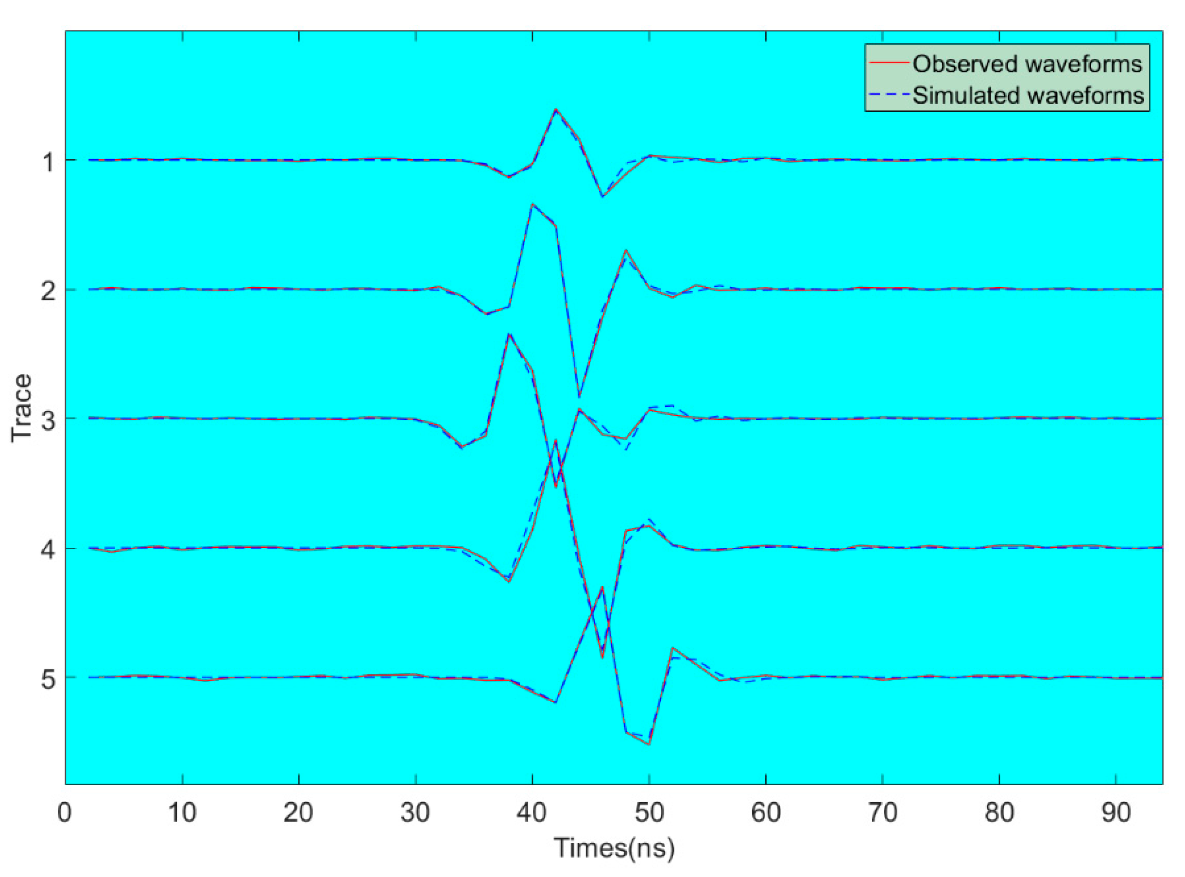
The vertical component of the electrical field is the recorded synthetic observational data which contains a total of 20 waveforms traces. Gaussian-distributed data uncertainties are added to the waveform data. The average signal-to-noise ratio is set to 25. A transmitter at depths of 3 m in the left borehole generates five waveform traces as Figure 3 shows. Blue dotted curves and red curves represent noise-free waveforms and noisy waveforms, respectively. The signal-to-noise ratios from the top are 8, 15, 24, 32 and 40, respectively. As can be seen from picture 3, the matching of waveforms from top to bottom gradually becomes better between the Noise-free waveforms and noisy waveforms.

For the time-lapse inversion, ${\mathit{m}}_{T1}$ represents the initial model at time $T_1$. We designed a perturbation in initial model ${\mathit{m}}_{T1}$ to obtain the monitor model ${\mathit{m}}_{T2}$, which simulated the monitor model at observational time $T_2$. Compared with ${\mathit{m}}_{T1}$, there was a high region of the relative dielectric permittivity near the surface in ${\mathit{m}}_{T2}$. ${\mathit{m}}_{T1}$, ${\mathit{m}}_{T2}$ and the perturbation as shown in Figure 4.

Before the inversion, we first needed to sample the priori probability density that generated the reference model ${\mathit{m}}_{T1}$. Figure 5 shows five sampling models generated from the priori probability density; each of them is different.

We used the extended Metropolis algorithm to obtain an a posteriori probability density. Figure 6 shows five inversion models that are generated from the posteriori probability density at $T_1$. We can see that the extended Metropolis algorithm obtained an effective inversion result. The inversion models contain the main features of ${\mathit{m}}_{T1}$. It is clear that relatively high dielectric permittivity structures are located at the bottom of the model and lower dielectric permittivity structures stay at the top of the model. In addition, Figure 7 shows the five waveform traces of a transmitter at depths of 3 m in the left borehole simulated by an a posteriori model. The simulated waveforms are consistent with observed waveforms.

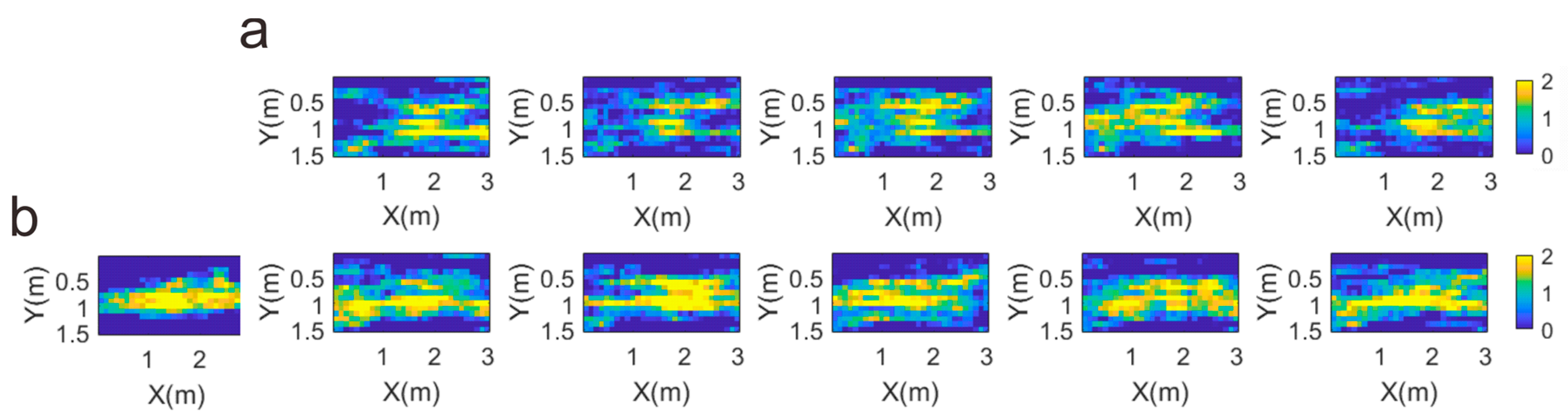
In the double difference strategy, to invert the mode ${\mathit{m}}_{T2}$, we selected a result of a posteriori sample as an initial model for the second inversion. In addition, we used the initial model to calculate forward data instead of observational data in the second inversion. Unlike the full sampling method in the first inversion, we used the sequential Gibbs algorithm to sample only the target area in the second inversion. In order to compare the inversion effect of local sampling, we set up a group of full sampling models for comparison. The results are shown in Figure 8. They clearly demonstrate that the local sampling performs better in the target area.

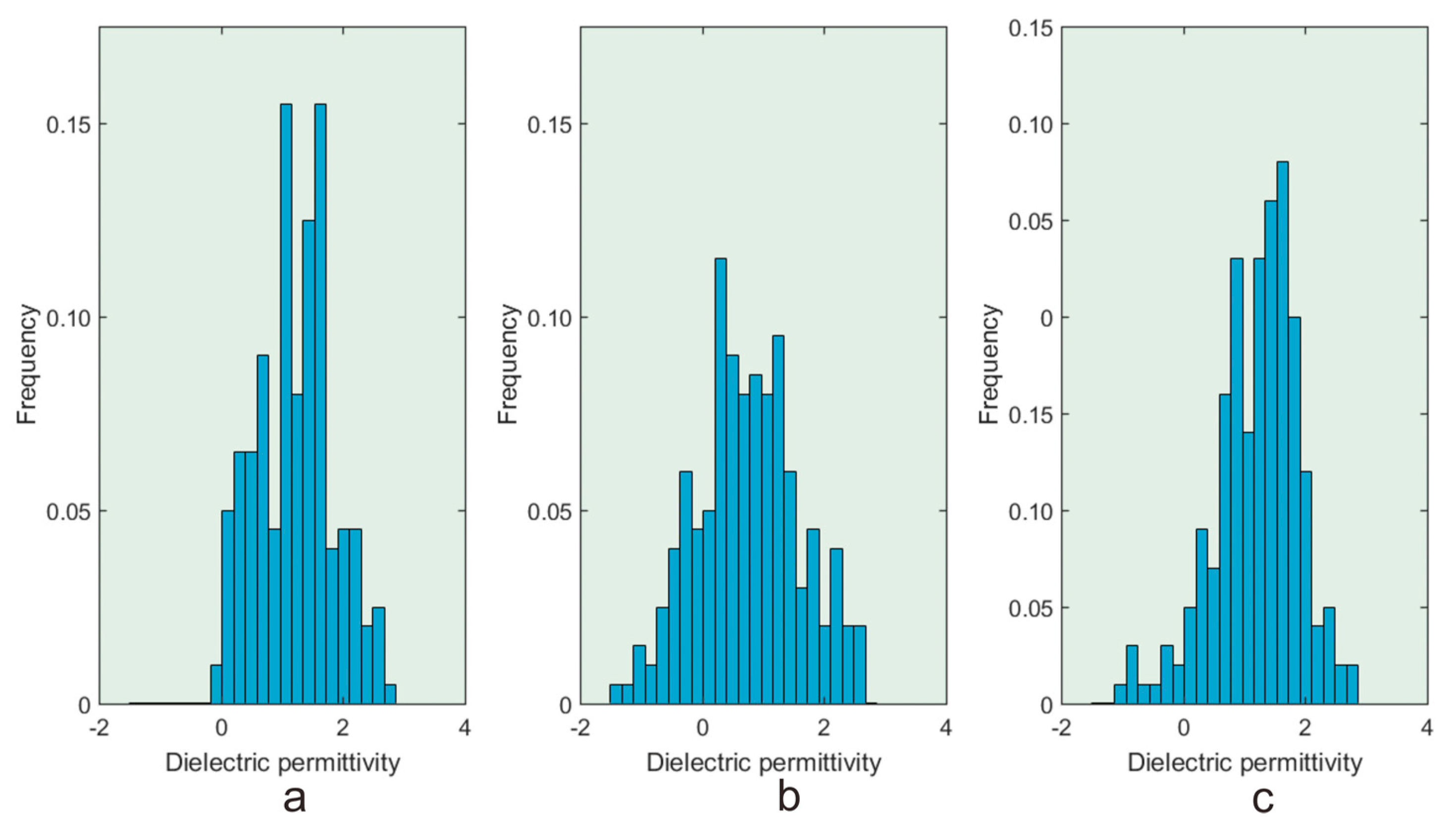
In order to analyze the disturbance location from the inversion results, we enlarged the target area in Figure 9. The first picture in Figure 9b is the designed perturbation model. It shows that Figure 9a is far from the designed perturbation model, while Figure 9b reflects the characteristics of the designed perturbation model. Furthermore, we made a statistical analysis of the target area; the histogram of the statistical data is shown in Figure 10; the specific mean and variance are shown in

Table 1. Statistical analysis of different methods of the target area.

Method	Mean	Variance
Design perturbation	1.25	0.43
All sampling	0.75	0.72
Local sampling	1.21	0.47

.

Figure 10a–c is the distribution of the designed perturbation, all sampling, and local sampling, respectively. It is obvious that the local sampling histogram is more similar to the design perturbation model. From Table 1, the mean and variance of local sampling is closer to the design perturbation model. It proves the effectiveness of the local sampling MCMC method.

4. Conclusions

This paper proposes a general framework for time-lapse inversion based on the MCMC method, which combines the extended Metropolis algorithm with a double difference strategy. In the double difference strategy, the result of the first inversion is taken as the initial model and forward data are used instead of observational data, using full-waveform data to invert the relative dielectric permittivity based on Maxwell’s equations. The waveform data are able to infer the model parameters effectively. In the extended Metropolis algorithm, sequential Gibbs sampling is used as a black box algorithm for sampling a priori probability density. This method can implement local sampling, which only samples the target area, reducing the influence of the non-target area. This makes the inversion result more accurate. The synthetic time-lapse GPR shows that, compared with full sampling, local sampling can obviously improve the resolution of the target region. It should be noted that we do a perfect assume about measured error and modeling error. We mainly consider the data uncertainties. It is a limitation of our current method.

References

- Rasol, M.A.; Pérez-Gracia, V.; Solla, M.; Pais, J.C.; Fernandes, F.M.; Santos, C. An experimental and numerical approach to combine Ground Penetrating Radar and computational modeling for the identification of early cracking in cement concrete pavements. NDT E Int. 2020, 115, 102293. [Google Scholar] [CrossRef]
- Solla, M.; Lagüela, S.; Riveiro, B.; Lorenzo, H. Non-destructive testing for the analysis of moisture in the masonry arch bridge of Lubians (Spain). Struct. Control. Health Monit. 2013, 20, 1366–1376. [Google Scholar] [CrossRef]
- Cui, T.J.; Chew, W.C.; Aydiner, A.A.; Chen, S.Y. Inverse scattering of two-dimensional dielectric objects buried in a lossy earth using the distorted Born iterative method. IEEE Trans. Geosci. Remote Sens. 2001, 39, 339–346. [Google Scholar]
- Zhou, H.; Sato, M. Subsurface cavity imaging by crosshole borehole radar measurements. IEEE Trans. Geosci. Remote Sens. 2004, 42, 335–341. [Google Scholar] [CrossRef]
- Qin, H.; Xie, X. Design and test of an improved dipole antenna for detecting enclosure structure defects by cross-hole gpr. IEEE J. Sel. Top. Appl. Earth Obs. Remote Sens. 2015, 9, 108–114. [Google Scholar] [CrossRef]
- Ernst, J.R.; Maurer, H.; Green, A.G.; Holliger, K. Full-waveform inversion of crosshole radar data based on 2-D finite-difference time-domain solutions of Maxwell’s equations. IEEE Trans. Geosci. Remote Sens. 2007, 45, 2807–2828. [Google Scholar] [CrossRef]
- Looms, M.C.; Jensen, K.H.; Binley, A.; Nielsen, L. Monitoring unsaturated flow and transport using cross-borehole geophysical methods. Vadose Zone J. 2008, 7, 227–237. [Google Scholar] [CrossRef] [Green Version]
- Binley, A.; Looms, M.C.; Doetsch, J.; Nielsen, L.; Jensen, K.H. Comparing plume characteristics inferred from cross-borehole geophysical data. Vadose Zone J. 2012, 11, 1–10. [Google Scholar]
- Güting, N.; Vienken, T.; Klotzsche, A.; van der Kruk, J.; Vanderborght, J.; Caers, J.; Vereecken, H.; Englert, A. High resolution aquifer characterization using crosshole GPR full-waveform tomography: Comparison with direct-push and tracer test data. Water Resour. Res. 2017, 53, 49–72. [Google Scholar] [CrossRef]
- Tarantola, A.; Valette, B. Inverse problems = quest for information. J. Geophys. 1982, 50, 159–170. [Google Scholar]
- Hansen, T.M.; Journel, A.G.; Tarantola, A.; Mosegaard, K. Linear inverse Gaussian theory and geostatistics. Geophysics 2006, 71, R101–R111. [Google Scholar] [CrossRef]
- Mosegaard, K. Resolution analysis of general inverse problems through inverse Monte Carlo sampling. Inverse Probl. 1998, 14, 405–426. [Google Scholar] [CrossRef]
- Devaney, A.J. Geophysical diffraction tomography. IEEE Trans. Geosci. Remote Sens. 1984, GRS-22, 3–13. [Google Scholar] [CrossRef]
- Hunziker, J.; Laloy, E.; Linde, N. Bayesian full-waveform tomography with application to crosshole ground penetrating radar data. Geophys. J. Int. 2019, 218, 913–931. [Google Scholar] [CrossRef]
- Qin, H.; Vrugt, J.A.; Xie, X.; Zhou, Y. Improved characterization of underground structure defects from two-stage Bayesian inversion using crosshole GPR data. Autom. Constr. 2018, 95, 233–244. [Google Scholar] [CrossRef] [Green Version]
- Mosegaard, K.; Tarantola, A. Monte Carlo sampling of solutions to inverse problems. J. Geophys. Res. 1995, 100, 431–447. [Google Scholar] [CrossRef]
- Hansen, T.M.; Cordua, K.C.; Mosegaard, K. Inverse problems with non-trivial priors-efficient solution through sequential Gibbs sampling. Comput. Geosci. 2012, 16, 593–611. [Google Scholar] [CrossRef] [Green Version]
- Hansen, T.M.; Mosegaard, K.; Cordua, K.S. Using geostatisticsto describe complex a priori information for inverse problems. In Geostatistics; Ortiz, J.M., Emery, X., Eds.; Gecamin Ltd.: Santiago, Chile, 2008; Volume 1. [Google Scholar]
- Hansen, T.; Cordua, K.; Looms, M.; Mosegaard, K. SIPPI: A matlab toolbox for sampling the solution to inverse problems with complex prior information. Part 2, Application to cross hole GPR tomography. Comput. Geosci. 2013, 52, 481–492. [Google Scholar] [CrossRef] [Green Version]
- Hansen, T.M.; Cordua, K.S.; Zunino, A.; Mosegaard, K. Probabilistic integration of geo-information. In Integrated Imaging of the Earth: Theory and Applications; Wiley: Hoboken, NJ, USA, 2016; Volume 218, pp. 93–116. [Google Scholar]
- Gomez-Hernandez, J.; Journel, A. Joint sequential simulation of multi-Gaussian fields. In Geostatistics Troia, Proceedings of the 4th International Geostatics Congress; Soares, A., Ed.; Kluwer Academic Publishers: Dordrecht, The Netherlands, 1 January 1993; Volume 92, pp. 85–94. [Google Scholar]
- Journel, A.; Zhang, T. The necessity of a multiple-point prior model. Math. Geol. 2006, 38, 591–610. [Google Scholar] [CrossRef]
- Moghadas, D.; Vrugt, J.A. The influence of geostatistical prior modeling on the solution of DCT-based Bayesian inversion: A case study from Chicken Creek catchment. Remote Sens. 2019, 11, 1549. [Google Scholar] [CrossRef] [Green Version]
- Remy, N.; Boucher, A.; Wu, J. Applied Geostatistics with SGeMS: A User’s Guide; Cambridge University Press: Cambridge, UK, 2008. [Google Scholar]
- Balkaya, C.; Akcıg, Z.; Gokturkler, G. A comparison of two travel-time tomography schemes for crosshole radar data: Eikonal-equation-based inversion versus ray-based inversion. J. Environ. Eng. Geophys. 2010, 15, 203–218. [Google Scholar] [CrossRef]
- Qin, H.; Wang, Z.; Tang, Y.; Geng, T. Analysis of Forward Model, Data Type, and Prior Information in Probabilistic Inversion of Crosshole GPR Data. Remote Sens. 2021, 13, 215. [Google Scholar] [CrossRef]
- Klotzsche, A.; van der Kruk, J.; Meles, G.A.; Doetsch, J.A.; Maurer, H.; Linde, N. Full-waveform inversion of cross-hole ground-penetrating radar data to characterize a gravel aquifer close to the Thur River, Switzerland. Near Surf. Geophys. 2010, 8, 635–649. [Google Scholar] [CrossRef]
- Cordua, K.S.; Hansen, T.M.; Mosegaard, K. Monte Carlo full-waveform inversion of crosshole GPR data using multiple-point geostatistical a priori information. Geophysics 2012, 77, H19–H31. [Google Scholar] [CrossRef] [Green Version]
- Waldhauser, F.; Ellsworth, W.L. A double-difference earthquake location algorithm: Method and application to the northern Hayward fault, California. Bull. Seismol. Soc. Am. 2000, 90, 1353–1368. [Google Scholar] [CrossRef]
- Huang, X.; Jakobsen, M.; Eikrem, K.S.; Nævdal, G. Target-oriented inversion of time-lapse seismic waveform data. Commun. Comput. Phys. 2020, 28, 249–275. [Google Scholar]
- Taflove, A.; Hagness, S.C. Computational Electrodynamics the Finite-Difference Time-Domain Method, 2nd ed.; Artech House: Boston, MA, USA, 2000. [Google Scholar]
- Yee, K.S. Numerical solution of initial boundary value problems involving Maxwell’s equations in isotropic media. IEEE Trans. Antennas Propag. 1966, AP-14, 302–307. [Google Scholar]
- Meles, G.A.; van der Kruk, J.; Greenhalgh, S.A.; Ernst, J.R.; Maurer, H.; Green, A.G. A new vector waveform inversion algorithm for simultaneous updating of conductivity and permittivity parameters from combination crosshole/borehole-to-surface GPR data. IEEE Trans. Geosci. Remote. Sens. 2010, 48, 3391–3407. [Google Scholar] [CrossRef]
- Routh, P.; Palacharla, G.; Chikichev, I.; Lazaratos, S. Full wavefield inversion of time-lapse data for improved imaging and reservoir characterization. SEG Expand. Abstr. 2012, 1–6. [Google Scholar] [CrossRef]
- Asnaashari, A.; Brossier, R.; Garambois, S.; Audebert, F.; Thore, P.; Virieux, J. Time-lapse seismic imaging using regularized full waveform inversion with a prior model:which strategy? Geophys. Prospect. 2015, 63, 78–98. [Google Scholar] [CrossRef]
- Peterson, J.E. Pre-inversion correction and analysis of radar tomographic data. J. Environ. Eng. Geophys. 2001, 6, 1–18. [Google Scholar] [CrossRef]
- Irving, J.D.; Knight, R.J. Effect of antennas onvelocity estimates obtained from crosshole GPR data. Geophysics 2005, 70, K39–K42. [Google Scholar] [CrossRef] [Green Version]
- Liu, T.; Klotzsche, A.; Pondkule, M. Radius estimation of subsurface cylindrical objects from ground-penetrating-radar data using full-waveform inversion. Geophysics 2018, 83, H43–H54. [Google Scholar] [CrossRef]
- Jazayeri, S.; Kazemi, N.; Kruse, S. Sparse blind deconvolution of ground penetrating radar data. IEEE Trans. Geosci. Remote Sens. 2019, 57, 3703–3712. [Google Scholar] [CrossRef]
Figure 1.
The double difference strategy. , are the corresponding observational data at different times ,. The models and are the inversion result at time ,. The result of time-lapse inversion can be obtained by subtracting from .
Figure 2.
Recording geometry; sources (red crosses) and receivers (black dots) are represented by a connecting black line.
Figure 3.
Noise-free waveforms and noisy waveforms: the signal-to-noise ratios from the top are 8, 15, 24, 32 and 40, respectively.
Figure 4.
Initial model , monitor model , and the perturbation.
Figure 5.
Five sampling models of the priori probability density.
Figure 6.
Five inversion models of the posterior probability density.
Figure 7.
Five waveform traces. Blue dotted curves: simulated waveforms calculated on a posteriori model. Red curves: the observed waveform data.
Figure 8.
(a) Full sampling inversion model of , and (b) the perturbation of the full sampling inversion. (c) Local sampling inversion model of , and (d) the perturbation of the local sampling inversion.
Figure 9.
(a) Target area of all sampling methods, and (b) target area of local sampling methods.
Figure 10.
(a) The design perturbation model histogram, (b) perturbation of all sampling histograms, and (c) perturbation of local sampling histogram.