
Identification of the Yield of Camellia oleifera Based on Color Space by the Optimized Mean Shift Clustering Algorithm Using Terrestrial Laser Scanning


Abstract
:
1. Introduction
2. Materials and Methods
2.1. Study Area
2.2. Framework of This Research
2.3. Point Cloud Acquisition and Processing
2.4. Measurement of Field Data
2.5. Identification of Oil Tea Fruits Point Clouds
2.6. Clustering Method for Oil Tea Fruits
2.7. Algorithm Accuracy Assessment
3. Results
3.1. Point Cloud Separation Results
3.2. Clustering Analysis
4. Discussion
4.1. Point Cloud Acquisition
4.2. Clustering Algorithm for Oil Tea Fruit Identification
4.3. Uncertainty, Limitations, and Prospects
5. Conclusions
Author Contributions
Funding
Institutional Review Board Statement
Informed Consent Statement
Data Availability Statement
Conflicts of Interest
References
- Zhang, S.; Li, X. Hypoglycemic activity in vitro of polysaccharides from Camellia oleifera Abel. seed cake. Int. J. Biol. Macromol. 2018, 115, 811–819. [Google Scholar] [CrossRef] [PubMed]
- Yeh, W.; Ko, J.; Huang, W.; Cheng, W.; Yang, H. Crude extract of Camellia oleifera pomace ameliorates the progression of nonalcoholic fatty liver disease via decreasing fat accumulation, insulin resistance and inflammation. Br. J. Nutr. 2019, 123, 508–515. [Google Scholar] [CrossRef] [PubMed]
- Lili, L.; Cheng, X.; Teng, L.; Wang, Y.; Dong, X.; Chen, L.; Zhang, D.; Peng, W. Systematic Characterization of Volatile Organic Components and Pyrolyzates from Camellia oleifera Seed Cake for Developing High Value-added Products. Arab. J. Chem. 2017, 11, 802–814. [Google Scholar] [CrossRef]
- Chen, Y.; Yang, C.; Chang, M.; Ciou, Y.; Huang, Y. Foam Properties and Detergent Abilities of the Saponins from Camellia oleifera. Int. J. Mol. Sci. 2010, 11, 4417–4425. [Google Scholar] [CrossRef] [PubMed] [Green Version]
- Ye, Y.; Guo, Y.; Luo, Y. Anti-Inflammatory and Analgesic Activities of a Novel Biflavonoid from Shells of Camellia oleifera. Int. J. Mol. Sci. 2012, 13, 12401–12411. [Google Scholar] [CrossRef]
- Zhu, J.; Zhu, Y.; Jiang, F.; Xu, Y.; Ouyang, J.; Yu, S. An integrated process to produce ethanol, vanillin, and xylooligosaccharides from Camellia oleifera shell. Carbohydr. Res. 2013, 382, 52–57. [Google Scholar] [CrossRef]
- Ma, B.; Huang, Y.; Nie, Z.; Qiu, X.; Su, D.; Wang, G.; Yuan, J.; Xie, X.; Wu, Z. Facile synthesis of Camellia oleifera shell-derived hard carbon as an anode material for lithium-ion batteries. RSC Adv. 2019, 9, 20424–20431. [Google Scholar] [CrossRef] [Green Version]
- Xu, T.; Cui, K.; Chen, J.; Wang, R.; Wang, X.; Chen, L.; Zhang, Z.; He, Z.; Liu, C.; Tang, W.; et al. Biodiversity of Culturable Endophytic Actinobacteria Isolated from High Yield Camellia oleifera and Their Plant Growth Promotion Potential. Agriculture 2021, 11, 1150. [Google Scholar] [CrossRef]
- Tu, J.; Chen, J.; Zhou, J.; Ai, W.; Chen, L. Plantation quality assessment of Camellia oleifera in mid-subtropical China. Soil Tillage Res. 2019, 186, 249–258. [Google Scholar] [CrossRef]
- Ye, H.-L.; Chen, Z.-G.; Jia, T.-T.; Su, Q.-W.; Su, S.-C. Response of different organic mulch treatments on yield and quality of Camellia oleifera. Agric. Water Manag. 2020, 245, 106654. [Google Scholar] [CrossRef]
- Murat, O.; Bulent, T.; Tuncay, D.; Erkan, B. An Effective Yield Estimation System Based on Blockchain Technology. IEEE Trans. Eng. Manag. 2020, 67, 1157–1168. [Google Scholar] [CrossRef]
- Wulfsohn, D.; Zamora, F.A.; Téllez, C.P.; Lagos, I.Z.; García-Fiñana, M. Multilevel systematic sampling to estimate total fruit number for yield forecasts. Precis. Agric. 2012, 13, 256–275. [Google Scholar] [CrossRef]
- Michael, M.; Kevin, T.; Jesslyn, B. Optimizing a remote sensing production efficiency model for macro-scale GPP and yield estimation in agroecosystems. Remote Sens. Environ. 2018, 217, 258–271. [Google Scholar] [CrossRef]
- Liu, Y.; Wang, J.; Dong, J.; Wang, S.; Ye, H. Variations of Vegetation Phenology Extracted from Remote Sensing Data over the Tibetan Plateau Hinterland during 2000–2014. J. Meteorol. Res. 2020, 34, 786–797. [Google Scholar] [CrossRef]
- Tian, F.; Brandt, M.; Liu, Y.Y.; Verger, A.; Tagesson, T.; Diouf, A.A.; Rasmussen, K.; Mbow, C.; Wang, Y.; Fensholt, R. Remote sensing of vegetation dynamics in drylands: Evaluating vegetation optical depth (VOD) using AVHRR NDVI and in situ green biomass data over West African Sahel. Remote Sens. Environ. 2016, 177, 265–276. [Google Scholar] [CrossRef] [Green Version]
- Sun, S.; Li, C.; Chee, P.W.; Paterson, A.H.; Jiang, Y.; Xu, R.; Robertson, J.S.; Adhikari, J.; Shehzad, T. Three-dimensional photogrammetric mapping of cotton bolls in situ based on point cloud segmentation and clustering. ISPRS J. Photogramm. Remote Sens. 2020, 160, 195–207. [Google Scholar] [CrossRef]
- Horng, G.-J.; Liu, M.-X.; Chen, C.-C. The Smart Image Recognition Mechanism for Crop Harvesting System in Intelligent Agriculture. IEEE Sens. J. 2019, 20, 2766–2781. [Google Scholar] [CrossRef]
- Xing, S.; Lee, M.; Lee, K.-K. Citrus Pests and Diseases Recognition Model Using Weakly Dense Connected Convolution Network. Sensors 2019, 19, 3195. [Google Scholar] [CrossRef] [Green Version]
- Moskal, L.M.; Zheng, G. Retrieving Forest Inventory Variables with Terrestrial Laser Scanning (TLS) in Urban Heterogeneous Forest. Remote Sens. 2012, 4, 1–20. [Google Scholar] [CrossRef] [Green Version]
- Schneider, F.D.; Leiterer, R.; Morsdorf, F.; Gastellu-Etchegorry, J.P.; Lauret, N.; Pfeifer, N.; Schaepman, M.E. Simulating imaging spectrometer data: 3D forest modeling based on LiDAR and in situ data. Remote Sens. Environ. 2014, 152, 235–250. [Google Scholar] [CrossRef]
- Lian, X.; Dai, H.; Ge, L.; Cai, Y. Assessment of a house affected by ground movement using terrestrial laser scanning and numerical modeling. Environ. Earth Sci. 2020, 79, 2181–2185. [Google Scholar] [CrossRef]
- Tong, X.; Liu, X.; Chen, P.; Liu, S.; Luan, K.; Li, L.; Liu, S.; Liu, X.; Xie, H.; Jin, Y.; et al. Integration of UAV-Based Photogrammetry and Terrestrial Laser Scanning for the Three-Dimensional Mapping and Monitoring of Open-Pit Mine Areas. Remote Sens. 2015, 7, 6635–6662. [Google Scholar] [CrossRef] [Green Version]
- Yang, H.; Xu, X.; Xu, W.; Neumann, I. Terrestrial Laser Scanning-Based Deformation Analysis for Arch and Beam Structures. IEEE Sens. J. 2017, 17, 4605–4611. [Google Scholar] [CrossRef]
- Xia, C.; Wang, L.; Chung, B.-K.; Lee, J.-M. In Situ 3D Segmentation of Individual Plant Leaves Using a RGB-D Camera for Agricultural Automation. Sensors 2015, 15, 20463–20479. [Google Scholar] [CrossRef] [PubMed]
- Yun, T.; Jiang, K.; Li, G.; Eichhorn, M.P.; Fan, J.; Liu, F.; Chen, B.; An, F.; Cao, L. Individual tree crown segmentation from airborne LiDAR data using a novel Gaussian filter and energy function minimization-based approach. Remote Sens. Environ. 2021, 256, 112307. [Google Scholar] [CrossRef]
- Polat, N.; Uysal, M. An investigation of tree extraction from UAV-based photogrammetric dense point cloud. Arab. J. Geosci. 2020, 13, 846–854. [Google Scholar] [CrossRef]
- Ebrahimi, A.; Czarnuch, S. Automatic Super-Surface Removal in Complex 3D Indoor Environments Using Iterative Region-Based RANSAC. Sensors 2021, 21, 3724. [Google Scholar] [CrossRef]
- Orozco-Del-Castillo, M.; Cárdenas-Soto, M.; Ortiz-Alemán, C.; Couder-Castañeda, C.; Urrutia-Fucugauchi, J.; Trujillo-Alcántara, A. A texture-based region growing algorithm for volume extraction in seismic data. Geophys. Prospect. 2017, 65, 97–105. [Google Scholar] [CrossRef] [Green Version]
- Li, B.; Jiang, G.; Shao, W. Color correction based on point clouds alignment in the logarithmic RGB space. Vis. Comput. 2015, 31, 257–270. [Google Scholar] [CrossRef]
- Xu, X.; Yang, H.; Neumann, I. A feature extraction method for deformation analysis of large-scale composite structures based on TLS measurement. Compos. Struct. 2018, 184, 591–596. [Google Scholar] [CrossRef]
- Moreno, R.; Graña, M.; Madani, K.; Ramik, D. Image segmentation on spherical coordinate representation of RGB colour space. IET Image Proc. 2018, 6, 1275–1283. [Google Scholar] [CrossRef]
- Zigh, E.; Kouninef, B.; Kadiri, M. Removing Shadows Using RGB Color Space in Pairs of Optical Satellite Images. J. Indian Soc. Remote Sens. 2017, 45, 431–441. [Google Scholar] [CrossRef]
- Prema, C.E.; Vinsley, S.S.; Suresh, S. Multi Feature Analysis of Smoke in YUV Color Space for Early Forest Fire Detection. Fire Technol. 2016, 52, 1319–1342. [Google Scholar] [CrossRef]
- Cho, W.; Jang, J.; Koschan, A.; Abidi, M.A.; Paik, J. Hyperspectral face recognition using improved inter-channel alignment based on qualitative prediction models. Opt. Express. 2016, 24, 27637–27662. [Google Scholar] [CrossRef]
- Yılmaztürk, F. Full-automatic self-calibration of color digital cameras using color targets. Opt. Express. 2011, 19, 18164–18174. [Google Scholar] [CrossRef]
- Czerniawski, T.; Sankaran, B.; Nahangi, M.; Haas, C.; Leite, F. 6D DBSCAN-based segmentation of building point clouds for planar object classification. Autom. Constr. 2018, 88, 44–58. [Google Scholar] [CrossRef]
- Wu, G.; Zhu, Q.; Huang, M.; Guo, Y.; Qin, J. Automatic recognition of juicy peaches on trees based on 3D contour features and colour data. Biosyst. Eng. 2019, 188, 1–13. [Google Scholar] [CrossRef]
- Tzortzis, G.; Likas, A. The MinMax k-Means clustering algorithm. Pattern Recognit. 2014, 47, 2505–2516. [Google Scholar] [CrossRef]
- Ferraz, A.; Saatchi, S.; Mallet, C.; Meyer, V. Lidar detection of individual tree size in tropical forests. Remote Sens. Environ. 2016, 183, 318–333. [Google Scholar] [CrossRef]
- Schmitt, M.; Shahzad, M.; Zhu, X.X. Reconstruction of individual trees from multi-aspect TomoSAR data. Remote Sens. Environ. 2015, 165, 175–185. [Google Scholar] [CrossRef] [Green Version]
- Lang, F.; Yang, J.; Yan, S.; Qin, F. Superpixel Segmentation of Polarimetric Synthetic Aperture Radar (SAR) Images Based on Generalized Mean Shift. Remote Sens. 2018, 10, 1592. [Google Scholar] [CrossRef] [Green Version]
- Gao, Y.; Yang, J.; Guo, L. Nonlocal oriented method for image denoising. Opt. Eng. 2011, 50, 030502. [Google Scholar] [CrossRef] [Green Version]
- Ji, J.; Li, X.-Y. Unsupervised synthetic aperture radar image segmentation with superpixels in independent space based on independent component analysis. J. Appl. Remote Sens. 2014, 8, 083682. [Google Scholar] [CrossRef]
- Tiegen, P.; Yinhua, W.; Tihua, W. Mean shift algorithm equipped with the intersection of confidence intervals rule for image segmentation. Pattern Recognit. Lett. 2007, 28, 268–277. [Google Scholar] [CrossRef]
- Yu, W.; Tian, X.; Hou, Z.; Zha, Y.; Yang, Y. Multi-scale mean shift tracking. IET Comput. Vision. 2015, 9, 110–123. [Google Scholar] [CrossRef]
- Kumar, P.; Dick, A. Adaptive earth movers distance-based Bayesian multi-target tracking. IET Comput. Vision. 2013, 7, 246–257. [Google Scholar] [CrossRef]
- Ortiz-Coder, P.; Sánchez-Ríos, A. An Integrated Solution for 3D Heritage Modeling Based on Videogrammetry and V-SLAM Technology. Remote Sens. 2020, 12, 1529. [Google Scholar] [CrossRef]
- Errington, A.F.C.; Daku, B.L.F. Temperature Compensation for Radiometric Correction of Terrestrial LiDAR Intensity Data. Remote Sens. 2017, 9, 356. [Google Scholar] [CrossRef] [Green Version]
- Thomas, V.; Treitz, P.; McCaughey, J.H.; Morrison, I. Mapping stand-level forest biophysical variables for a mixedwood boreal forest using lidar: An examination of scanning density. Can. J. For. Res. 2006, 36, 34–47. [Google Scholar] [CrossRef]
- Hopkinson, C.; Chasmer, L.; Young-Pow, C.; Treitz, P. Assessing forest metrics with a ground-based scanning lidar. Can. J. For. Res. 2004, 34, 573–583. [Google Scholar] [CrossRef] [Green Version]
- Ning, X.; Li, F.; Tian, G.; Wang, Y. An efficient outlier removal method for scattered point cloud data. PLoS ONE 2018, 13, e0201280. [Google Scholar] [CrossRef] [PubMed] [Green Version]
- Yan, L.; Liu, H.; Tan, J.; Li, Z.; Chen, C. A Multi-Constraint Combined Method for Ground Surface Point Filtering from Mobile LiDAR Point Clouds. Remote Sens. 2017, 9, 958. [Google Scholar] [CrossRef] [Green Version]
- Le, Q.; Liscio, E. A comparative study between FARO Scene and FARO Zone 3D for area of origin analysis. Forensic Sci. Int. 2019, 301, 166–173. [Google Scholar] [CrossRef] [PubMed]
- Dandois, J.P.; Baker, M.; Olano, M.; Parker, G.G.; Ellis, E.C. What is the Point? Evaluating the Structure, Color, and Semantic Traits of Computer Vision Point Clouds of Vegetation. Remote Sens. 2017, 9, 355. [Google Scholar] [CrossRef] [Green Version]
- Lu, N.; Zhou, J.; Han, Z.; Li, D.; Cao, Q.; Yao, X.; Tian, Y.; Zhu, Y.; Cao, W.; Cheng, T. Improved estimation of aboveground biomass in wheat from RGB imagery and point cloud data acquired with a low-cost unmanned aerial vehicle system. Plant Methods 2019, 15, 1–16. [Google Scholar] [CrossRef] [Green Version]
- Wen, S. Display gamut comparison with number of discernible colors. J. Electron. Imaging 2006, 15, 043001. [Google Scholar] [CrossRef]
- Li, Q.; Cheng, X. Comparison of Different Feature Sets for TLS Point Cloud Classification. Sensors 2018, 18, 4206. [Google Scholar] [CrossRef] [Green Version]
- Duong, T.; Beck, G.; Azzag, H.; Lebbah, M. Nearest neighbour estimators of density derivatives, with application to mean shift clustering. Pattern Recognit. Lett. 2016, 80, 224–230. [Google Scholar] [CrossRef]
- Öztekin, I.; Long, N.M.; Badre, D. Optimizing Design Efficiency of Free Recall Events for fMRI. J. Cognit. Neurosci. 2010, 22, 2238–2250. [Google Scholar] [CrossRef] [Green Version]
- Ray, W.D. Multiple Regression and Analysis of Variance. J. Oper. Res. Soc. 2017, 28, 611–612. [Google Scholar] [CrossRef]
- Xu, J.-X.; Ma, J.; Tang, Y.-N.; Wu, W.-X.; Shao, J.-H.; Wu, W.-B.; Wei, S.-Y.; Liu, Y.-F.; Wang, Y.-C.; Guo, H.-Q. Estimation of Sugarcane Yield Using a Machine Learning Approach Based on UAV-LiDAR Data. Remote Sens. 2020, 12, 2823. [Google Scholar] [CrossRef]
- LJarron, L.R.; Coops, N.C.; MacKenzie, W.H.; Tompalski, P.; Dykstra, P. Detection of sub-canopy forest structure using airborne LiDAR. Remote Sens. Environ. 2020, 244, 111770–111782. [Google Scholar] [CrossRef]
- Arnó, J.; Escolà, A.; Masip, J.; Rosell-Polo, J.R. Influence of the scanned side of the row in terrestrial laser sensor applications in vineyards: Practical consequences. Precis. Agric. 2015, 16, 119–128. [Google Scholar] [CrossRef] [Green Version]
- Renard, F.; Voisin, C.; Marsan, D.; Schmittbuhl, J. High resolution 3D laser scanner measurements of a strike-slip fault quantify its morphological anisotropy at all scales. Geophys. Res. Lett. 2006, 33, 4305-1–4305-4. [Google Scholar] [CrossRef] [Green Version]
- Jackson, S.S.; Bishop, M.J.; Leese, D.L.; Lord, E.M. High-resolution 3D laser imaging of various surfaces in minefields and implications for surface modeling. Proc. SPIE Int. Soc. Opt. Eng. 2005, 5794, 857–865. [Google Scholar] [CrossRef]
- Hämmerle, M.; Höfle, B. Effects of Reduced Terrestrial LiDAR Point Density on High-Resolution Grain Crop Surface Models in Precision Agriculture. Sensors 2014, 14, 24212–24230. [Google Scholar] [CrossRef] [Green Version]
- Khazaei, J.; Naghavi, M.; Jahansouz, M.; Salimi-Khorshidi, G. Yield Estimation and Clustering of Chickpea Genotypes Using Soft Computing Techniques. Agron. J. 2008, 100, 1077–1087. [Google Scholar] [CrossRef]
- Genta, G.; Minetola, P.; Barbato, G. Calibration procedure for a laser triangulation scanner with uncertainty evaluation. Opt. Lasers Eng. 2016, 86, 11–19. [Google Scholar] [CrossRef]
- Wang, L.; Muralikrishnan, B.; Rachakonda, P.; Sawyer, D. Determining geometric error model parameters of a terrestrial laser scanner through two-face, length-consistency, and network methods. Meas. Sci. Technol. 2017, 28, 065016. [Google Scholar] [CrossRef]
- Liu, S.; Xu, D.; Li, Y.-F.; Shen, F.; Zhang, D.-P. Nanoliter Fluid Dispensing Based on Microscopic Vision and Laser Range Sensor. IEEE Trans. Ind. Electron. 2017, 64, 1292–1302. [Google Scholar] [CrossRef]
- Srinivasan, S.; Popescu, S.; Eriksson, M.; Sheridan, R.; Ku, N.-W.J.R.S. Terrestrial Laser Scanning as an Effective Tool to Retrieve Tree Level Height, Crown Width, and Stem Diameter. Remote Sens. 2015, 7, 1877–1896. [Google Scholar] [CrossRef] [Green Version]
- Zhang, Y.; Migliavacca, M.; Penuelas, J.; Ju, W. Advances in hyperspectral remote sensing of vegetation traits and functions. Remote Sens. Environ. 2020, 252, 112121–112126. [Google Scholar] [CrossRef]
- Axelsson, P. Processing of laser scanner data—Algorithms and applications. ISPRS J. Photogramm. Remote Sens. 1999, 54, 138–147. [Google Scholar] [CrossRef]
- Koetz, B.; Sun, G.; Morsdorf, F.; Ranson, K.J.; Kneubühler, M.; Itten, K.; Allgöwer, B. Fusion of imaging spectrometer and LIDAR data over combined radiative transfer models for forest canopy characterization. Remote Sens. Environ. 2007, 106, 449–459. [Google Scholar] [CrossRef]
- Ghamkhar, K.; Irie, K.; Hagedorn, M.; Hsiao, J.; Fourie, J.; Gebbie, S.; Hoyos-Villegas, V.; George, R.; Stewart, A.; Inch, C.; et al. Real-time, non-destructive and in-field foliage yield and growth rate measurement in perennial ryegrass (Lolium perenne L.). Plant Methods 2019, 15, 72. [Google Scholar] [CrossRef] [PubMed]
- Guan, H.; Yu, Y.; Ji, Z.; Li, J.; Zhang, Q. Deep learning-based tree classification using mobile LiDAR data. Remote Sens. Lett. 2015, 6, 864–873. [Google Scholar] [CrossRef]
- Chen, J.; Chen, Y.; Liu, Z. Classification of Typical Tree Species in Laser Point Cloud Based on Deep Learning. Remote Sens. 2021, 13, 4750. [Google Scholar] [CrossRef]
- Rehush, N.; Abegg, M.; Waser, L.T.; Brändli, U.-B. Identifying Tree-Related Microhabitats in TLS Point Clouds Using Machine Learning. Remote Sens. 2018, 10, 1735. [Google Scholar] [CrossRef] [Green Version]
- Xi, Z.; Hopkinson, C.; Chasmer, L. Filtering Stems and Branches from Terrestrial Laser Scanning Point Clouds Using Deep 3-D Fully Convolutional Networks. Remote Sens. 2018, 10, 1215. [Google Scholar] [CrossRef] [Green Version]


| Total Number of Oil Tea Fruits | Mean | Maximum | Minimum | Average Radius of Oil Tea Fruits (cm) |
|---|---|---|---|---|
| 19,066 | 241 | 593 | 38 | 2.0 |
| Color Space | Attribute Characteristics | Maximum Value | Minimum Value |
|---|---|---|---|
| RGB | R | 255 | 200 |
| G | 250 | ||
| B | 250 | ||
| YUV | Y | 160 | |
| U | 220 | ||
| V | 220 |
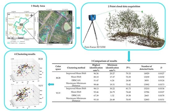
| Color Space | Clustering Method | Highest Detection Rate/% | Minimum Detection Rate/% | Number of Detected Fruits | D | |
|---|---|---|---|---|---|---|
| RGB | Improved Mean Shift | 96.56 | 20.27 | 79.33 | 14,929 | 0.0127 |
| Mean Shift | 89.19 | 17.37 | 70.29 | 13,039 | 0.0150 | |
| DBSCAN | 51.47 | 6.24 | 24.80 | 3855 | 0.0124 | |
| Maximum–Minimum Distance | 98.48 | 19.31 | 75.42 | 13,992 | 0.0173 | |
| YUV | Improved Mean Shift | 98.13 | 30.22 | 81.73 | 15,210 | 0.0134 |
| Mean Shift | 93.46 | 26.79 | 74.68 | 13,786 | 0.0127 | |
| DBSCAN | 67.39 | 1.32 | 19.38 | 2665 | 0.0178 | |
| Maximum–Minimum Distance | 93.18 | 26.48 | 70.95 | 12,893 | 0.0151 |
Publisher’s Note: MDPI stays neutral with regard to jurisdictional claims in published maps and institutional affiliations. |
© 2022 by the authors. Licensee MDPI, Basel, Switzerland. This article is an open access article distributed under the terms and conditions of the Creative Commons Attribution (CC BY) license (https://creativecommons.org/licenses/by/4.0/).
Share and Cite
Tang, J.; Jiang, F.; Long, Y.; Fu, L.; Sun, H. Identification of the Yield of Camellia oleifera Based on Color Space by the Optimized Mean Shift Clustering Algorithm Using Terrestrial Laser Scanning. Remote Sens. 2022, 14, 642. https://doi.org/10.3390/rs14030642
Tang J, Jiang F, Long Y, Fu L, Sun H. Identification of the Yield of Camellia oleifera Based on Color Space by the Optimized Mean Shift Clustering Algorithm Using Terrestrial Laser Scanning. Remote Sensing. 2022; 14(3):642. https://doi.org/10.3390/rs14030642
Chicago/Turabian StyleTang, Jie, Fugen Jiang, Yi Long, Liyong Fu, and Hua Sun. 2022. "Identification of the Yield of Camellia oleifera Based on Color Space by the Optimized Mean Shift Clustering Algorithm Using Terrestrial Laser Scanning" Remote Sensing 14, no. 3: 642. https://doi.org/10.3390/rs14030642