
An Automatic Procedure for Forest Fire Fuel Mapping Using Hyperspectral (PRISMA) Imagery: A Semi-Supervised Classification Approach


1
Department of Astronautical, Electrical and Energy Engineering, University of Rome “La Sapienza”, 00185 Rome, Italy
2
School of Aerospace Engineering, University of Rome “La Sapienza”, 00138 Rome, Italy
*
Author to whom correspondence should be addressed.
Remote Sens. 2022, 14(5), 1264; https://doi.org/10.3390/rs14051264
Submission received: 1 February 2022
/
Revised: 26 February 2022
/
Accepted: 1 March 2022
/
Published: 4 March 2022
(This article belongs to the Special Issue Remote Sensing and Smart Forestry)
Abstract
:Natural vegetation provides various benefits to human society, but also acts as fuel for wildfires. Therefore, mapping fuel types is necessary to prevent wildfires, and hyperspectral imagery has applications in multiple fields, including the mapping of wildfire fuel types. This paper presents an automatic semisupervised machine learning approach for discriminating between wildfire fuel types and a procedure for fuel mapping using hyperspectral imagery (HSI) from PRISMA, a recently launched satellite of the Italian Space Agency. The approach includes sample generation and pseudolabelling using a single spectral signature as input data for each class, unmixing mixed pixels by a fully constrained linear mixing model, and differentiating sparse and mountainous vegetation from typical vegetation using biomass and DEM maps, respectively. Then the procedure of conversion from a classified map to a fuel map according to the JRC Anderson Codes is presented. PRISMA images of the southern part of Sardinia, an island off Italy, were considered to implement this procedure. As a result, the classified map obtained an overall accuracy of 87% upon validation. Furthermore, the stability of the proposed approach was tested by repeating the procedure on another HSI acquired for part of Bulgaria and we obtained an overall stability of around 84%. In terms of repeatability and reproducibility analysis, a degree of confidence greater than 95% was obtained. This study suggests that PRISMA imagery has good potential for wildfire fuel mapping, and the proposed semisupervised learning approach can generate samples for training the machine learning model when there is no single go-to dataset available, whereas this procedure can be implemented to develop a wildfire fuel map for any part of Europe using LUCAS land cover points as input.
Keywords:
forests; fires; fuel map; hyperspectral; LUCAS; machine learning; PRISMA; pseudolabels; SVM classifier; sample generation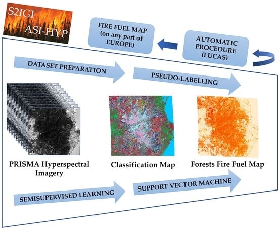
1. Introduction
Fire is a significant ecological disturbance that threatens ecosystem sustainability worldwide, specifically in Mediterranean regions. Bond et al. [1] consider fire to be like the biggest “herbivore” on Earth [1]. Over the last five decades, researchers have paid much attention to the ecological impacts of fire. Fire behaviour helps determine the impact of fire to a considerable extent. Fire behaviour has different ecological impacts, and also helps us to determine the optimal suppression strategy for any given fire [2,3,4,5]. Fire intensity and rate of spread are two important aspects of fire behaviour that are affected, among other factors, by the load, type, and continuity of fuel [6]. Fuel types vary; for instance, Pinus halepensis is more flammable [3] due to the highly flammable resins and oils, producing high-intensity fires. At the same time, fuel continuity and fuel load relate to the percentage of the surface covered by vegetation—in other words, by potential fuels [6]. The accuracy and effectiveness of any tool for the simulation of fire behaviour or fire risk assessment depend on the accuracy and availability of data related to the vegetation ecosystem [3,4]. Spatially and thematically accurate vegetation cover is critical for the suppression and prevention of fire in fire-prone areas and ecosystems [7]. Goodenough et al. [8] have compared forest classification accuracies between EO-1’s Hyperion and ALI sensors and Landsat 7 ETM+ and concluded that hyperspectral sensors provide better discrimination with greater accuracy in comparison with multispectral sensors in several forest types. The potential of wildfire fuel mapping using hyperspectral data of Hyperion was evaluated by Yoon et al. [9] almost a decade ago and they concluded that Hyperion imagery has good potential for wildfire fuel mapping. Mapping boreal forest fuel types for interior Alaska, Smith et al. [10] used AVIRIS-NG hyperspectral data with 80% accuracy, while LANDFIRE’s Existing Vegetation Type product derived from Landsat-8 had 33% accuracy. For the same region of interest, hyperspectral data simulated using Sentinel-2 was used to map boreal forest fuel type with 89% accuracy, which was better than the accuracy obtained using multispectral Sentinel-2 [11]. A review was conducted by Sander et al. [12] on hyperspectral remote sensing of fire. The authors commented that hyperspectral data had proven utility in the temporal stage of the fire disturbance continuum, including prefire applications, i.e., in exact fuel type and condition assessment. Also, they added that, until 2018, there were only airborne hyperspectral data, and upcoming spaceborne missions like PRISMA, EnMAP, and HyspIRI will provide opportunities to explore further the linkages between ecosystem properties and fires at a regional to global scale. In this work, the feasibility and maturity of hyperspectral imagery from PRISMA (PRecursore IperSpettrale della Missione Applicativa), launched by the Italian Space Agency (ASI) in 2019, have been evaluated for mapping wildfire fuel types. After the commissioning phase, access to the data was granted to users in early June 2020. PRISMA is an on-demand mission, and the available data in the archive are limited [13].
Machine learning algorithms have become a vital tool in modern hyperspectral image analysis, especially in land cover classification, because of their unprecedented predictive power [14,15]. However, the accuracy of the machine learning-based classification depends entirely on the dataset. Therefore, annotated datasets have become a crucial pre-condition for developing and evaluating machine learning-based classifications. However, due to the heterogeneity of remote sensing measurements and tasks, there is no single go-to dataset that could serve the purpose of standardized pretraining and benchmarking [16,17]. Thus, a dataset was prepared by pseudolabelling the pixels or spectral signatures collected from the PRISMA image for mapping wildfire fuel types.
Another challenge in machine learning is the selection of a suitable machine learning classifier for a particular task among the various machine learning methods. Selecting based on accuracy is also tricky since the accuracy of ML algorithms depends upon various factors such as dataset pattern, size of training data, training parameters, etc. In such cases, an optimal algorithm can be selected considering the specific case, classes to be mapped, nature and size of training data, and predictor variables. The classification accuracy of supervised machine learning classifiers varies with the size of the training samples [18]. One study concluded that SVM accuracy decreased by 6.25% when using just 15 training samples instead of 100 for each class, and SVMs were less sensitive to training data size than other machine learning models. Thus, a support vector machine (SVM) classifier was chosen to perform the classification of vegetation types considering all the factors mentioned above, specifically the size of training data [19,20]. Classification of the mixed pixels in hyperspectral data is another vital process to be considered. In our case, a fully constrained linear mixing model was used to assign mixed pixels to their appropriate category. In the framework of EFFIS (European Forest Fire Information System) and FUELMAP projects under the Joint Research Centre (JRC), a categorization of the fuel types available in Europe was carried out and correlated with Anderson fuel models (1982) [21,22].
Therefore, this paper presents an automatic procedure for mapping wildfire fuel types using PRISMA hyperspectral imagery in a semisupervised machine learning approach. This work was started under the project S2IGI (an integrated system for forest fire management) funded by the Regional Administration of Sardinia under the POR (Programma Operativo Regionale) FESR (Fondo Europeo di Sviluppo Regionale) Sardinia and improved under the project ASI-HYP, funded by the Italian Space Agency. The main objectives of this work are (1) to develop an automatic procedure for wildfire fuel mapping, using PRISMA hyperspectral imagery and the land cover data from regional/national portals as input and (2) to correlate the fuel types to Anderson fuel models, more appropriately incorporating secondary classifications (sparse/dense, plains/mountains, etc.), if necessary, to extract the attributes of fuel models such as the fuel load (t/ha) for the living and dead components of the vegetation, the height of the fuel (litter) to the ground, extinction humidity (%), flame height (m), and propagation rate (m/s). In this paper, initially, the procedure developed to map fuel types using the vegetation map from the regional portal of Sardinia is presented, and the possibility of this procedure being extended to any part of Europe by using the LUCAS database as input is also explained. Section 2 describes the PRISMA data and methods used, and Section 3 describes the stepwise procedure of dataset preparation and fuel mapping. Section 4 represents and discusses the results obtained. Finally, Section 5 summarizes the conclusions of this work.
2. Data and Methods
This section explains the PRISMA hyperspectral data, the region of interest, and the methods implemented in this work. Collecting in situ data for the whole island is impossible, so a procedure is proposed to prepare a dataset given one known pixel as input, referring to the maps available from regional/national portals. Samples for the dataset were generated by pseudolabelling the unlabelled pixels available in the image using the methods described in this section. This process involves guided image filtering, Jeffries–Matusita spectral angle mapper, and k-means clustering methodology. Finally, the samples generated were implemented to train the support vector machine classifier.
2.1. Study Area
This work is part of the project funded for Sardinia. Sardinia, an island in the south of Italy and the second-largest island in the Mediterranean Sea, as shown in Figure 1, has frequent fires. In the last decade, 1008 fires per year ere recorded in Sardinia alone, which is 20% of the total fires at the national level [23]. This is a windy island with somewhat rainy winters, hot sunny summers, and an average temperature range of 10 °C in winter (January/February) to 24–25 °C in summer (July/August).
As an example, an image of 10 October 2021 on the southern part of this Mediterranean island was selected from the archived data shown in Figure 1. This image comprises Monte Arcosu Forest, one of the immense holm oak forests of the Mediterranean region, which is east of Cagliari. The region of interest is hilly with an altitude of around 800 m and a total area of 32 km2. The primary vegetation in this forest is holm oak (Quercion ilicis) and mastic shrubs of two different families (Ericion arboreae and Oleo ceratonian). The highest areas have low vegetation, specifically meadows of two different families (Teucrion mari and Periballio-Trifolion subterranei), whereas the lowest areas (around 200–300 m altitude) have evergreen broadleaved trees (Quercetalia ilicis) [24,25].
2.2. PRISMA Data
In this work, hyperspectral imagery from the PRISMA satellite as used to map vegetation fuel types. PRISMA has launched a new era of hyperspectral imaging spectroscopy. This imaging spectrometer can capture a continuum of spectral bands with 400 to 2500 nm at a spatial resolution of 30 m. The sensor counts 173 bands in the shortwave infrared (SWIR) within 920–2500 nm, and 66 bands are in the visible near-infrared (VNIR) portion of the spectrum (400–1010 nm). The widths and spectral sampling intervals are ≤12 nm. A panchromatic camera providing a single-band (400–700 nm) image at 5 m spatial resolution is also onboard the ASI’s satellite. PRISMA is an on-demand mission; the data in the archive (https://prisma.asi.it, accessed on 15 January 2022) are limited but imagery for the required location can be acquired upon request [13].
ASI delivers PRISMA products in four levels: L1, L2B, L2C, and L2D. L1 data contain top of atmosphere (TOA) radiometrically and geometrically calibrated hypercube and panchromatic radiance images. L2B contains geolocated and atmospherically corrected hypercube and panchromatic radiance images. L2C contains geolocated and atmospherically corrected hypercube and panchromatic reflectance images, whereas L2D also contains similar images but they are geolocated and geocoded. In addition, the L1 product comprises cloud and land cover maps, whereas L2C and L2D products have atmospheric constituent maps such as water vapour, aerosols, and thin cloud optical thickness. For detailed information on PRISMA product specifications, please refer to the PRISMA product specifications document on https://prisma.asi.it (accessed on 15 January 2022).
2.3. Reference Data
Reference data are necessary to train the machine learning model and validate the predicted output. Usually, remote sensing specialists conduct field campaigns to collect ground truth data as reference data for validation, but field campaigns were not performed due to COVID-19. During the pandemic, researchers around the world have tried other alternatives, such as using readily available maps/ground truth data collected by volunteers or airborne data as a reference [26,27,28]. This work used the Nature system map (Sardinia) accessed through the Sardinia geoportal and CORINE land cover (CLC) of 2018 and Grassland maps accessed from Copernicus Land Monitoring Service as reference data. The Nature System map (Carta della natura) prepared by Italian National Institute for Environmental Protection and Research (ISPRA) is more detailed and accurate [29,30] than the CLC, having an accuracy of around 85% [31]. Among these three, CLC has a total area coverage of 5.8 Mkm2 and 32 European Environmental Agency countries and seven cooperating countries are under coverage [32]. Two validation studies show that it has achieved an accuracy of 85% [32], which encouraged us to use CLC for reference data.
The Nature System map has 93 classes for Sardinia; CLC has 44 land cover types [31,32] at the third level for Europe, whereas the grasslands map shows the presence/absence of grasslands. For the region of interest, the nature system map had 43 classes, among which 18 fuel types were selected, as shown in Figure 2a, depending upon the area covered by each class. These three maps were used to differentiate and cross-check the pixels corresponding to trees, shrubs, and grasslands. Three classes, namely coniferous vegetation, holm oak trees, and grasslands near the Mediterranean coast, were verified using CLC and grassland maps.
Figure 2 shows the Nature System, CLC, and grassland maps that were referred to for input and later for validation of output. Classes were mainly chosen from Nature System, and grassland maps and CLC were used to cross-check in case of any confusion in selecting the appropriate pixels. Classes are shown in Figure 2a: 1—Halophyte vegetation with the dominance of annual succulent Chenopodiaceae, 2—Matorral of evergreen oaks, 3—Matorral with olive and mastic, 4—Matorral of junipers, 5—Low olive and mastic shrubs, 6—Low shrubs (from Calicotome family), 7—Formations of Euphorbia dendroides, 8—Garrigues and meso-Mediterranean silicicole spots, 9—Garrigues and calciculous mesomediterraneal spots, 10—Arid Mediterranean meadows, 11—Mediterranean grassland (including Mediterranean and postcultural sub-Mediterranean vegetation), 12—Riparian Mediterranean ash forests, 13—Tamarisk and oleander, 14—Tyrrhenian Cork, 15—Sardinian Leccete (Holm Oak), 16—Vegetation of reeds and similar species, 17—Coniferous vegetation, and 18—Eucalyptus plantations. Figure 2b shows the CLC map with five selected classes: 311—Broadleaved forest, 312—Coniferous forest, 313—Mixed forest, 321—Natural grasslands, and 323—Sclerophyllous vegetation. Figure 2c shows the pixels covered by grasslands, especially in urban areas.
2.4. Methods Implemented
This work implemented a sequence of methods to pseudolabel the pixels available in the image using a single spectral signature as input. This section explains the need for a particular method in this proposed procedure.
2.4.1. Guided Image Filtering
The guided filter is an edge-preserving smoothing algorithm that could smooth out the fine details of the input image while retaining the sharp edges. Fine details could be noise (for example, a random pattern with a zero mean) or texture, such as a repeated pattern with a regular structure. Applications of guided filtering include denoising, image mapping, dehazing and compression, and tone mapping of high-dynamic-range (HDR) images [33,34,35,36]. Guidance images can be obtained by performing a principal component analysis (PCA). The first three principal components were considered a colour guidance image for the guided filtering process.
2.4.2. Jeffries–Matusita Spectral Angle Mapper
Spectral angle mapper (SAM) is one of the most popular techniques in hyperspectral data analysis as it measures the spectral angle between the reference spectra and the target spectrum. SAM can detect the intrinsic properties of materials in terms of spectral angle, but is insensitive to shade and illumination effects. Thus, different materials/vegetation types with similar spectral shapes and offsets are classified only with difficulty [37]. SAM was used in combination with the stochastic divergence measures to overcome the insensitivity limitations mentioned above [38]. Thus, the Jeffries–Matusita (JM) distance measure was combined with SAM to identify similar spectra. The JM distance between two spectra measures the average distance between the spectra. The exponential factor involved in this method gives an exponentially decreasing weight to increasing separation between the spectra, and this approach overcomes the limitation of transformed divergence [39].
Furthermore, JM distance measures bandwise information between spectral vectors [40,41]. To identify similar spectra, JM-SAM (TAN) was used in which the deterministic SAM was combined with the stochastic JM distance using the tangent function as it projects the target spectrum and reference spectrum perpendicularly. This method considers the geometrical aspects (angle, distance) and band information between the spectral vectors. As a result, the least separable distance between the spectral vectors at each band and the minor spectral angle between the vectors is considered the best match [40,42].
2.4.3. K-Means Clustering
A proper unsupervised clustering technique can cluster data where the number of clusters (K) is either known, presumed, or indicated beforehand. The members of each group have similar characteristics and properties. This study used this technique in the dataset preparation process to collect true and false data for binary classification problems. As per the suggestion of Nguyen et al. [43,44], it would be better if the number of clusters K is greater than the number of expected or actual classes, so three clusters were formed since it is a binary classification. The k-means algorithm was carried out using the Machine Learning Toolbox of MATLAB. As a result, three groups were formed with similar spectral signatures, different spectral signatures, and very noisy spectral signatures, respectively [3,43,44].
2.4.4. Support Vector Machine for HSI Classification
There are numerous supervised learning-based algorithms in the artificial intelligence field that can be applied for classification [45,46]. In the current framework, SVM (with radial basis function, RBF) was applied because of its reputation in training datasets to achieve high accuracy irrespective of the size of the dataset and outstanding generalization capability. This method works on statistical learning theory and the structural risk minimization principle [47]. The optimal separating hyperplane with the maximum margin between the classes will be found using the strategy of this classifier using the training samples located at the edge of the class distribution [46]. Initially, the optimal values were found by hyperparameter optimization in the classification learner app of MATLAB but observed that it is slowly leading to overfitting. So, the Bayesian optimization technique was applied to optimize a few parameters such as sigma, box constraint, etc. Then, the SVM model developed was allowed to find posterior probabilities by training parameters of an additional sigmoid function to map the outputs into probabilities. Constructing a classifier to produce a posterior probability is helpful in practical recognition situations. For example, a posterior probability allows for making decisions using the utility model. Posterior probabilities play an essential role in making an overall decision when the classifier is limited to making a small part of an overall decision [47,48,49].
2.4.5. Linear Mixing Model
A linear mixing model is necessary when the pixel comprises materials with different reflectance properties and the spectral variability within the scene results from varying proportions of the endmembers [50,51]. The spectrum of the mixed pixel can be represented as a linear combination of component spectra (endmembers) in LMM. The weight of each endmember (abundance) is proportional to the fraction of the pixel area covered by the endmember [14,52]. If there are L spectral bands, the spectra of the endmembers and the pixel spectrum can be represented by L-dimensional vectors.
2.4.6. JRC—Anderson Fuel Models Correlation
In the EFFIS and FUELMAP projects under JRC [22,53,54], the correlation of vegetation types in Europe to Anderson fuel models was obtained. Under these projects, fuel of 42 types (as shown in Table 1) available in Europe were categorized into nine groups: Peat bogs (FT_1 and FT_2), Grasslands (FT_3 to FT_6), Shrublands (FT_7 to FT_12), Transitional Shrubland/Forest (FT_13 to FT_19), Coniferous Forest (FT_20 to FT_28), Broadleaved Forest (FT_29 to FT_34), Mixed Forest (FT_35 to FT_38), Aquatic Vegetation (FT_39 to FT_41), and Agroforestry areas (FT_42). Then, the correlation of fuel types to the fuel models of Anderson (1982) [54] was made, as shown in Table 1. This work generated a fuel map by referring to these JRC Anderson Codes. This correlation was used in this work to correlate the classified fuel types to Anderson codes [22,53,54,55].
3. Proposed Framework
The steps followed to develop a wildfire fuel map that involves various steps, viz., preprocessing, pixels extraction, dataset preparation by pseudolabelling, machine learning algorithm details, unmixing, further classification of fuel types, and fuel map, are illustrated in the flowchart in Figure 3. Details of the process are described in the following subsections.
3.1. Preprocessing
Level 2C and Level 1 products from the PRISMA archive with minimal cloud cover were considered. The atmospheric correction of the level 2C products is based upon inverting the radiative transfer model, i.e., minimizing a cost function representing the difference between the simulated spectrum and the measured one. The MODTRAN model performed the simulations, and they are stored as a lookup table (LUT) to speed up the inversion. Georeferencing of the image was carried out using the PRISMAread tool [56] developed by the National Research Council of Italy on R software. This tool imports the original data provided in he5 format and converts them to ENVI or GTiff format as per the requirements. The latitude and longitude files containing geographic latitude/longitude values (WGS-84 datum) are provided in the he5 file. Further details on the PRISMAread tool can be accessed from https://irea-cnr-mi.github.io/prismaread/ (accessed on 15 January 2022).
Further details about the mission and products are available in the PRISMA products specification document. Level 2C was considered for the fuel mapping, whereas the level 1 product provides a basic land cover map with classes, viz., water pixel, snow pixel, bare soil, cropland, forest, wetland, and urban component used to classify vegetation pixels from nonvegetated pixels, as shown in Figure 4a. Thus, the processing time was reduced by applying the proposed procedure only to vegetation areas.
Removing noisy bands is a required preprocessing step for most hyperspectral remote sensing applications. In this work, noisy bands were removed by giving a threshold in the algorithm, i.e., bands with more than 20% noisy pixels (omitting the bands with noisy lines, as shown in Figure 4b) were removed from the hypercube. In this image, 197 spectral bands in the range of 400 to 2500 nm, with a spectral bandwidth within ~9–12 nm, were extracted from Level 2C data to perform the classification, removing 36 noisy and water absorption bands.
Few bands of the PRISMA image contain noisy lines, as shown in Figure 4b; filling those lines was one of the essential preprocessing steps. Neglecting this step will cause these lines to show up in the final classification map. In this work, those lines were filled by interpolating the nearest neighbour pixels in a linear way.
3.2. Pixel Extraction
Pixel’s extraction of the HSI (Hyperspectral Image) is one of the imperative preprocessing mechanisms. It assists in handling the data and implementing the machine learning algorithms giving it as input data, as shown in the flowchart (Figure 4). The individual elements in the HSI are pixels of which the spectra are formed as vectors. Nature system map, CLC, and grassland maps obtained from sources such as Sardinia Geoportal and Copernicus Land Monitoring Service as described in Section 2.3 were considered reference maps for input data. Pixels that correspond to fuel types were selected and inputted for dataset preparation. Figure 1 shows the points selected for each vegetation type to be classified.
Points marked in Figure 1 represents 1—Halophyte vegetation with the dominance of annual succulent Chenopodiaceae, 2—Matorral of evergreen oaks, 3—Matorral with olive and mastic, 4—Matorral of junipers, 5—Low olive and mastic shrubs, 6—Low shrubs (from Calicotome family), 7—Formations of Euphorbia dendroides, 8—Garrigues and meso-mediterranean silicicole spots, 9—Garrigues and calciculous mesomediterraneal spots, 10—Arid Mediterranean meadows, 11—Mediterranean grassland (including Mediterranean and postcultural sub-Mediterranean vegetation), 12—Riparian Mediterranean ash forests, 13—Tamarisk and oleander, 14—Tyrrhenian Cork, 15—Sardinian Leccete (Holm Oak), 16—Vegetation of reeds and similar species, 17—Coniferous vegetation, and 18—Eucalyptus plantations.
3.3. Dataset Preparation
The flowchart shown in Figure 5 illustrates the procedure followed to generate and pseudolabel the samples for the dataset preparation and is as follows:
Step 1: Preprocessing of PRISMA data was carried out as explained in Section 3.1.
Step 2: HSI was denoised using the guided image filtering technique explained in Section 2.4. It was performed in MATLAB software, giving the degree of smoothness parameter as 0.01.
Step 3: Spectral signatures corresponding to the pixels extracted following the procedure explained in Section 3.2. were collected for all 18 classes. Since one of the main objectives of this work is to create a dataset using a single spectral signature as input, only one pixel per class was extracted, and one spectral signature per class was considered.
Step 4: JM-SAM (TAN) was applied to collect similar and dissimilar spectral signatures from the image. This technique has provided us with a score map, with values ranging from lower to higher according to the similarity of the given spectral profile. The score map was used to extract similar profiles by visually inspecting them and giving a threshold, but an unsupervised clustering technique (K-means) was preferred to remove the threshold system.
Step 5: The K-means clustering technique was applied to JM-SAM (TAN) scores to cluster the obtained values into three groups. Though we need only two groups (similar and dissimilar), three groups were formed referring to the literature, as explained in Section 2.4.3.
Step 6: A dataset of 500 samples was planned for each class/fuel type by pseudolabelling, as shown in Figure 5. Spectral signatures corresponding to the pixels having up to 300 scores in group 1 (similar profiles) were collected and labelled as ‘1’, which refers to pure samples. Then, 200 spectral profiles were randomly collected using the scores of group 2 (dissimilar) and group 3 (noisy) and labelled as ‘0’, which refers to impure samples. This process of dataset preparation was repeated for each fuel type.
Step 7: This pseudolabelled dataset was used for training and testing the SVM model (one vs. all) for binary classification, so it was named a semisupervised learning approach.
3.4. Classification Algorithm Details
Support vector machine classifier was considered for training using the generated dataset on MATLAB R2021b with Machine Learning Toolbox. In addition, the accuracy implemented to assess the trained model performance is the ratio of correctly classified testing samples to the total number of testing samples. The procedure followed for training, testing, and predicting is as follows:
Step 1: The dataset was divided into two: 70% as a training dataset and 30% as a testing dataset.
Step 2: K-fold cross-validation was performed with k = 10 to fit the model with a minor error.
Step 3: Hyperparameters given for tuning are as follows: radial basis function as kernel, sigma of range [1e-5 1e+5], and box constraint of range [1e-5 1e+5].
Step 4: Defined hyperparameters were optimized with Bayesian optimization in MATLAB Statistical Tool Box.
Step 5: The SVM classifier model was trained using the optimal hyperparameters and RBF as the kernel.
Step 6: The SVM posterior probability model was trained using the trained SVM classifier model as input. This step created the score-to-posterior transformation function (sigmoid function) and computed posterior probabilities for the samples classified as the positive class.
Step 7: The cross-validation classification model was trained to perform 10-fold cross-validation and find the classification (kfoldLoss). For every class, less than 5% of classification loss was obtained.
Step 8: The trained SVM posterior probability model was validated using the testing dataset for accuracy. If the accuracy was greater than 0.95, the model was considered for prediction.
The same steps were repeated for every class, and the classes obtained as output from the SVM classifier are shown in Figure 6.
3.5. Further Classification
Concerning the JRC–Anderson correlation [Table 1], Anderson codes differ between sparse grassland and typical grassland. According to the EFFIS project, sparse grasslands will have 1.83 tons/hectare of biomass [54]. So, a biomass map was obtained from EU Copernicus and differentiated spare grasslands from grasslands. Figure 7 shows the classification of sparse grasslands (class 2) from grasslands (class 1).
3.6. Linear Unmixing
Fully constrained LMM was applied to unmix the unclassified pixels as per the method described in Section 2. Before unmixing, classes 1 to 18 were categorized into three groups, with forests containing classes 12, 14, 15, and 17, shrubs containing classes 1, 2, 3, 4, 5, 6, 7, 8, 9, 13, and 18, and grasslands containing classes 10, 11, and 16.
Then, unmixing was carried out to identify the percentage of forests, shrubs, and grasslands in each pixel. The value for each pixel was assigned by knowing the percentage of each group in a pixel. Accordingly, mixed pixels were classified into six classes: 111—pixel with 50% forests and 50% unvegetated area, 112—pixel with 50% shrubs and 50% unvegetated area, 113—pixel with 50% of grasslands and 50% unvegetated area, 123—pixel with 50% forests, 20% shrubs and 30% grasslands, 231—pixel with 50% shrubs, 20% grasslands and 30% forests, and 312—pixel with 50% grasslands, 20% forests and 30% shrubs. Figure 8 shows the classification map obtained from fully constrained LMM.
3.7. Fuel Mapping
By referring to the correlation of JRC and Anderson codes shown in Table 1, Anderson codes were assigned to the pixels of the classified map with respect to the fuel types tabulated in Table 2. For mixed pixels, whichever fuel type had a higher percentage of occupancy was given the Anderson code corresponding to that fuel type.
4. Results and Discussion
This section shows the final classification and fuel maps obtained from the proposed method and the validation details.
4.1. Classification and Fuel Map
As per the methodology in the previous section, the hyperspectral imagery of PRISMA in Monte Arcosu Forest was classified into 18 classes and six mixed-pixel classes, as shown in Figure 9. Details of classes are given in Section 3.2. It can be observed from the obtained maps that the significant fuel types available in this region of interest are fuel type 2 (evergreen oak), fuel type 15 (holm oak), and fuel type 5 (mastic scrubs/bushes), which is in alignment with the literature stating that this forest has these three vegetation types at different altitudes [24,25]. This region also contains Eucalyptus plantations (fuel type 18), which are highly flammable compared to the major cover of broadleaved forest. Eucalyptus plants contain a high concentration of volatile compounds and accumulate a larger amount of flammable litter from leaves and bark [57].
One of the main factors affecting fire behaviour is fuel distribution, but our understanding of the fuel density’s heterogeneity effect on fire behaviour is limited. A study conducted by Adam et al. [58] concluded that increased fuel density had decreased forward fire spread due to a combination of fuel discontinuities and increased fine-scale turbulent wind structures. In contrast, a decrease in local fuel continuity and wind entrainment into the forest canopy maintained near-surface wind speeds had driven fire spread. Considering this point, mixed pixels with partial vegetation must also be considered as fuel-containing pixels. In this work, mixed pixels were classified into six types, as explained in Section 3.6, among which class 111 (50% forests and 50% unvegetated area) showed a higher amount.
Figure 10 shows the wildfire fuel map obtained by following the procedure described in Section 3.7. The fuel map has values ranging from 1 to 10, representing the fuel models of Anderson’s classification. By associating the classified fuel types with standard fuel models, each fuel type in this map is correlated to the attributes of fuel models such as fuel load (t/ha) for the living and dead components of the vegetation, the height of the fuel (litter) from the ground, extinction humidity (%), flame height (m), and propagation rate (m/s) [54].
4.2. Validation
The classified map was validated using different sources, i.e., the Nature System map of Sardinia, CLC, and grasslands maps, accessed from regional/or EU Copernicus geoportals, as described in Section 2.2. Each class was validated by randomly taking 30 points to measure the classification accuracy, which is the ratio of correctly classified points to the total number of points.
Table 3 shows each class’s precision, recall, and F1 score. This image’s major fuel types (class 2, 5, and 15) obtained 86%, 86%, and 90% accuracy. Almost every class has an accuracy of above 80%, except class 1. It was observed that halophyte vegetation (class 1) is spread over the forest in small areas, but the reference map shows only near the Mediterranean coast, leading to less accuracy.
Performance metrics for each class were identified to check the accuracy of the machine learning model. Performance metrics include precision, recall, and F1 score. Therefore, these scores take false positives and false negatives into account together. Understanding the F1 score is intuitively not easy, but F1 is usually more beneficial than accuracy, especially if there is uneven class distribution. Accuracy works best if false positives and false negatives have similar costs. In the case of different false positives and false negatives, it is better to look at precision and Recall.
The validation details showed an overall accuracy of 87.10%, which is the ratio of correctly classified points for all classes to the total number of points. Due to the lack of recent reference/ground truth data to validate, the uncertainty of ±5% inaccuracy can be expected. An EFFIS pan-European fuel map was prepared using CLC with eight vegetation classes/fuel types with 250 m of spatial resolution and at an accuracy of around 85% [54]. A fuel map under the framework of the ArcFuel project was prepared using CLC and Landsat 7 data with eight fuel types at a resolution of 50 m; it obtained an accuracy of 76% at Italian pilot sites [59,60]. Comparison with other fuel products is problematic since regional fuel maps use many different classification systems [57].
4.3. Stability Analysis
In order to evaluate the robustness of the machine learning classifier algorithm, PRISMA hyperspectral imagery from another region of interest for different dates, i.e., 27 June 2021 and 31 July 2021, was selected from the archive for fuel mapping.
According to the Anderson fuel models, the fuel maps were developed for two dates. Figure 11a shows the fuel map developed for 27 June 2021 on the imagery acquired on Lazio (Rome) comprising Castel Porziano. Figure 11b shows the fuel map developed for 31 July 2021 and is slightly rotated from Figure 11a. Fuel values were assigned in the range of (1–10) for both the maps; the similarity between the maps can be observed.
Since Figure 11b is slightly rotated, a common region from both the images was selected for the stability analysis. Images covering Castel Porziano were clipped from both these images as shown in Figure 12a,b. The similarity between these two images can be observed from Figure 12 and the numerical values in Table 4.
The stability of a learning algorithm refers to the changes in the output of the system when we change the training dataset. Therefore, a learning algorithm is stable if the learned model does not change much when the training dataset is modified. For example, when selecting a training dataset from the same image in the PRISMA hyperspectral imagery classification problem, using cross-validation, a loss of less than 5% was obtained, which means it was 95% stable. However, this cannot be considered alone when the algorithm is developed for different images.
Mathematically, there are many types of stability analysis, such as hypothesis stability, cross-validation, etc. Here, cross-validation was performed between two fuel maps developed using images on the same region of interest but acquired on different dates.
Table 4 shows the number of pixels and the difference between two images for each fuel. The difference in the number of pixels ranged from <1% to 26% for specific classes. The significant difference between these two images is the number of bands. For example, the image taken on 31 July 2021 has a higher number of noisy bands (22) than the previous image (four), which was one of the reasons for the variation in stability. Also, the images were considered during the summer season of Italy, which explains the difference in vegetation. Considering these differences and the obtained percentages, it can be observed that the overall stability is around 80%.
4.4. Repeatability and Reproducibility Analysis
To evaluate the repeatability and reproducibility of the algorithm, an image (of 19 January 2022) from Bulgaria was selected since a fuel map acquired from the local authorities is available as a reference. The classification and fuel map were generated for this image with six classes, as shown in Table 5. The input for this image was taken from the specified reference map, as shown in Figure 13a.
Figure 13b shows the classification map with six classes and its corresponding fuel map in Figure 13c. Again, the fuel map based on PRISMA is clipped for the region of interest. Details of classes and the Anderson codes are given in Table 1.
The reference fuel map has fuel types assigned to only four fuel models (1, 2, 6, and 9). The majority of vegetation in this area is Black Pine (coniferous forest), followed by other fuel types, as shown in Table 1. This scenario is also similar to the PRISMA-based fuel map except that the fuel types assigned to fuel model 9 have sparse vegetation, which is inadequately classified due to the dark pixels in the hyperspectral data (as shown in RGB of the PRISMA image).
A detailed evaluation, including misclassifications, can be shown only by the confusion matrix in Table 6. A confusion matrix, created by considering 30 points for each category in the fuel map, obtained an overall accuracy of ≅~84%. It can be observed from the overall accuracies that the degree of confidence obtained was greater than 95%.
4.5. Extension of Procedure for Europe-Wide Fuel Mapping with LUCAS Database
Since this procedure considers one spectral signature as input, it can be implemented to map wildfire fuel types in any part of Europe. For demonstration purposes, an image covering the city of Calabria in the south of Italy was considered. The LUCAS (land use/cover area survey) points map was accessed from Copernicus Land Monitoring Services, which provides information about the land use and land cover of Europe. Forest/vegetation information is provided under the land cover classification systems, which is categorised into eight different types: A—Artificial Land, B—Cropland, C—Woodland, D—Shrubland, E—Grassland, F—Bare land, G—Water and H—Wetland. Each of these categories is further categorised into various types. Among them, the image considered for the fuel mapping contained six vegetation types: (1) C10 (Broadleaved Trees), (2) D10 (Shrubland with sparse tree cover), (3) C32 (Pine-dominated mixed vegetation), (4) E20 (Grass without tree/shrub cover), (5) C22 (Pine-dominated coniferous vegetation), and (6) C33 (Other mixed vegetation).
Considering the points from LUCAS as input and by overlapping, spectral signatures corresponding to those pixels were extracted. Then, the procedure described in this paper was followed to develop classification and fuel map as shown in Figure 14a,b, respectively. Thus, this automatic procedure can develop a wildfire fuel map on any part of Europe using LUCAS points as input.
4.6. Possible Applications of the Fuel Map
The procedure proposed in this work can be applied to any local region (such as a country or province) to create a custom fuel map using the local vegetation information. The dataset can be prepared following this proposed procedure if no local vegetation information/ground truth data are available. Researchers/policymakers/fire managers use fuel maps to study fire potential, fire behaviour, fire emissions, fire management, fire effects, land surface temperature [61], and ecosystem modelling [54]. In our ongoing project (S2IGI), the fuel map of the EFFIS project was used to calculate the fire danger hazard index [62] and to develop a wildfire vulnerability map [63]. These maps will be updated using the developed fuel map.
Due to the limited number of studies on wildfire fuel mapping using spaceborne hyperspectral data, this work could become an example demonstrating the feasibility and maturity of spaceborne hyperspectral data in the prevention and management of wildfires. Future developments of this work would be (1) to verify the procedure by associating fuel types to Scott–Burgan fuel models, including isobioclimatic conditions and (2) to apply a quantum support vector machine classifier as it can learn with fewer data [64].
5. Conclusions
In this article, an automatic wildfire fuel mapping procedure using machine learning on hyperspectral imagery from the PRISMA satellite has been put forward. All the necessary fuel types in the image covering the southern part of Sardinian Island were detected. However, there was no suitable dataset or literature available, so a semisupervised learning approach was proposed for fuel mapping. The support vector machine classifier was implemented to identify the fuel types using the posterior probabilities and obtained an overall accuracy of 87% by validation. The stability of the procedure and the machine learning model was checked by repeating the same procedure on HSI of PRISMA covering the west of Latium, Italy, and an overall stability of around 80% (considering the difference in images) was obtained. In a repeatability and reproducibility analysis using an image for Bulgaria, an overall accuracy of 84% was obtained. This procedure obtained a degree of confidence greater than 95% concerning repeatability and reproducibility analysis. Finally, the proposed procedure was applied to the image covering the city of Calabria in the south of Italy using LUCAS points map as input, which demonstrated that this procedure could be applied to any part of Europe for wildfire fuel mapping.
Author Contributions
Conceptualization, G.L. and R.U.S.; methodology, R.U.S. and G.L.; software, R.U.S.; validation, R.U.S., L.F. and G.L.; formal analysis, R.U.S. and G.L.; investigation, R.U.S.; resources, G.L. and L.F.; data curation, R.U.S., L.F., and G.L.; writing—original draft preparation, R.U.S.; writing—review and editing, R.U.S. and G.L.; visualization, R.U.S. and G.L.; supervision, G.L.; project administration, G.L.; funding acquisition, G.L. All authors have read and agreed to the published version of the manuscript.
Funding
This research was started under the project “S2IGI: An Integrated System for Prevention and Management of Wildfires,” funded by Regional Administration of Sardinia under the POR (Programma Operativo Regionale) FESR (Fondo Europeo di Sviluppo Regionale) Sardinia and improved under the project “ASI-HYP,” funded by the Italian Space Agency.
Institutional Review Board Statement
Not applicable.
Informed Consent Statement
Not applicable.
Data Availability Statement
Not applicable.
Acknowledgments
The authors would like to thank the Regional Administration of Sardinia and Italian Space Agency for the funding.
Conflicts of Interest
The authors declare no conflict of interest. The funders had no role in the design of the study; in the collection, analyses, or interpretation of data; in the writing of the manuscript, or in the decision to publish the results.
References
- Bond, W.J.; Keeley, J.E. Fire as a global ‘herbivore’: The ecology and evolution of flammable ecosystems. Trends Ecol. Evol. 2005, 20, 387–394. [Google Scholar] [CrossRef] [PubMed]
- Informazioni su Questo Libro. Available online: http://books.google.com (accessed on 15 September 2021).
- Vakalis, D.; Sarimveis, H.; Kiranoudis, C.; Alexandridis, A.; Bafas, G. A GIS based operational system for wildland fire crisis management I. Mathematical modelling and simulation. Appl. Math. Model. 2004, 28, 389–410. [Google Scholar] [CrossRef]
- Vakalis, D.; Sarimveis, H.; Kiranoudis, C.; Alexandridis, A.; Bafas, G. A GIS based operational system for wildland fire crisis management II. System architecture and case studies. Appl. Math. Model. 2004, 28, 411–425. [Google Scholar] [CrossRef]
- Keramitsoglou, I.; Kiranoudis, C.T.; Sarimvels, H.; Sifakis, N. A Multidisciplinary Decision Support System for Forest Fire Crisis Management. Environ. Manag. 2004, 33, 212–225. [Google Scholar] [CrossRef] [PubMed]
- Whelan, R.J. The Ecology of Fire-Developments since 1995 and Outstanding Questions Long-Term Trends in Flowering and Fruit Set in Banksia View Project Pollination of Diuris (Orchidaceae) View Project. 2009. Available online: https://www.researchgate.net/publication/30387859 (accessed on 15 September 2021).
- Barmpoutis, P.; Papaioannou, P.; Dimitropoulos, K.; Grammalidis, N. A Review on Early Forest Fire Detection Systems Using Optical Remote Sensing. Sensors 2020, 20, 6442. [Google Scholar] [CrossRef] [PubMed]
- Goodenough, D.; Dyk, A.; Niemann, K.; Pearlman, J.; Chen, H.; Han, T.; Murdoch, M.; West, C. Processing hyperion and ali for forest classification. IEEE Trans. Geosci. Remote Sens. 2003, 41, 1321–1331. [Google Scholar] [CrossRef]
- Yeosang, Y.; Yongseung, K. Application of Hyperion Hyperspectral Remote Sensing Data for Wildfire Fuel Map-ping. Korean J. Remote Sens. 2007, 23, 21–32. Available online: https://www.koreascience.or.kr/article/JAKO200712242534560.pdf (accessed on 28 November 2021).
- Smith, C.; Panda, S.; Bhatt, U.; Meyer, F. Improved Boreal Forest Wildfire Fuel Type Mapping in Interior Alaska Using AVIRIS-NG Hyperspectral Data. Remote Sens. 2021, 13, 897. [Google Scholar] [CrossRef]
- Badola, A.; Panda, S.; Roberts, D.; Waigl, C.; Bhatt, U.; Smith, C.; Jandt, R. Hyperspectral Data Simulation (Sentinel-2 to AVIRIS-NG) for Improved Wildfire Fuel Mapping, Boreal Alaska. Remote Sens. 2021, 13, 1693. [Google Scholar] [CrossRef]
- Veraverbeke, S.; Dennison, P.; Gitas, I.; Hulley, G.; Kalashnikova, O.; Katagis, T.; Kuai, L.; Meng, R.; Roberts, D.; Stavros, N. Hyperspectral remote sensing of fire: State-of-the-art and future perspectives. Remote Sens. Environ. 2018, 216, 105–121. [Google Scholar] [CrossRef]
- Niroumand-Jadidi, M.; Bovolo, F.; Bruzzone, L. Water Quality Retrieval from PRISMA Hyperspectral Images: First Experience in a Turbid Lake and Comparison with Sentinel-2. Remote Sens. 2020, 12, 3984. [Google Scholar] [CrossRef]
- Gewali, U.B.; Monteiro, S.T.; Saber, E. Machine Learning Based Hyperspectral Image Analysis: A Survey. February 2018. Available online: http://arxiv.org/abs/1802.08701 (accessed on 15 September 2021).
- Talukdar, S.; Singha, P.; Mahato, S.; Shahfahad; Pal, S.; Liou, Y.-A.; Rahman, A. Land-Use Land-Cover Classification by Machine Learning Classifiers for Satellite Observations—A Review. Remote Sens. 2020, 12, 1135. [Google Scholar] [CrossRef] [Green Version]
- Schmitt, M.; Ahmadi, S.A.; Hansch, R. There is No Data Like More Data–Current Status of Machine Learning Datasets in Remote Sensing. In Proceedings of the 2021 IEEE International Geoscience and Remote Sensing Symposium IGARSS, Brussels, Belgium, 11–16 July 2021; pp. 1206–1209. [Google Scholar]
- Sarvia, F.; De Petris, S.; Borgogno-Mondino, E. Mapping Ecological Focus Areas within the EU CAP Controls Framework by Copernicus Sentinel-2 Data. Agronomy 2022, 12, 406. [Google Scholar] [CrossRef]
- Foody, G.M.; Pal, M.; Rocchini, D.; Garzon-Lopez, C.X.; Bastin, L. The Sensitivity of Mapping Methods to Reference Data Quality: Training Supervised Image Classifications with Imperfect Reference Data. ISPRS Int. J. Geo-Inf. 2016, 5, 199. [Google Scholar] [CrossRef] [Green Version]
- Cervantes, J.; Garcia-Lamont, F.; Rodríguez-Mazahua, L.; Lopez, A. A comprehensive survey on support vector machine classification: Applications, challenges and trends. Neurocomputing 2020, 408, 189–215. [Google Scholar] [CrossRef]
- Archibald, R.; Fann, G. Feature Selection and Classification of Hyperspectral Images with Support Vector Machines. IEEE Geosci. Remote Sens. Lett. 2007, 4, 674–677. [Google Scholar] [CrossRef]
- Advance EFFIS Report on Forest Fires in Europe, Middle East and North Africa 2018; Publications Office of the European Union: Luxembourg, 2019. [CrossRef]
- Toukiloglou, P.; Eftychidis, G.; Gitas, I.; Tompoulidou, M. ArcFuel methodology for mapping forest fuels in Europe. In Proceedings of the First International Conference on Remote Sensing and Geoinformation of Environment, Paphos, Cyprus, 8–10 April 2013; Volume 8795. [Google Scholar] [CrossRef]
- European Commission, Joint Research Centre; San-Miguel-Ayanz, J.; Durrant, T.; Boca, R. Forest Fires in Europe, Middle East and North Africa 2020. 2021. Available online: https://data.europa.eu/doi/10.2760/059331 (accessed on 15 September 2021).
- Mossa, L.; Bacchetta, G.; Angiolino, C.; Ballero, M. A contribution to the floristic knowledge of the Monti del Sulcis: Monte Arcosu (S.W. Sardinia). Flora Mediterr. 2016, 6, 157–190. [Google Scholar]
- European Commission, Joint Research Centre. European Atlas of Forest Tree Species; San-Miguel-Ayanz, J., Caudullo, G., De Rigo, D., Mauri, A., Houston Durrant, T., Eds.; European Comission: Brussels, Belgium, 2022; Available online: https://data.europa.eu/doi/10.2760/233115 (accessed on 15 September 2021).
- Duveau, S. Frozen data? Polar research and fieldwork in a pandemic era. Polar Record 2021, 57, E34. [Google Scholar] [CrossRef]
- Jawak, S.D.; Andersen, B.N.; Pohjola, V.A.; Godøy; Hübner, C.; Jennings, I.; Ignatiuk, D.; Holmén, K.; Sivertsen, A.; Hann, R.; et al. SIOS’s Earth Observation (EO), Remote Sensing (RS), and Operational Activities in Response to COVID-19. Remote. Sens. 2021, 13, 712. [Google Scholar] [CrossRef]
- U.S. Global Development Lab. Guide for Adopting Remote Monitoring Approaches during COVID-19. Available online: https://www.usaid.gov/digital-development/covid19-remote-monitoring-guide (accessed on 15 September 2021).
- Santarsiero, V. A Remote Sensing Methodology to Assess the Abandoned Arable Land Using NDVI Index in Basili-cata Region. In Proceedings of the Computational Science and Its Applications–ICCSA 2021, Cagliari, Italy, 13–16 September 2021; pp. 695–703. [Google Scholar]
- Tucci, B.; Nolè, G.; Lanorte, A.; Santarsiero, V.; Cillis, G.; Scorza, F.; Murgante, B. Assessment and Monitoring of Soil Erosion Risk and Land Degradation in Arable Land Combining Remote Sensing Methodologies and RUSLE Factors. In Information for a Better World: Shaping the Global Future; Springer Science and Business Media LLC: Berlin/Heidelberg, Germany, 2021; pp. 704–716. [Google Scholar]
- EEA. Copernicus Land Monitoring Service 2020. Available online: https://land.copernicus.eu/ (accessed on 15 May 2020).
- Büttner, G. CORINE Land Cover and Land Cover Change Products. In Land Use and Land Cover Mapping in Europe; Manakos, I., Braun, M., Eds.; Springer Science and Business Media LLC: Dordrecht, Switzerland, 2014; Volume 18, pp. 55–74. [Google Scholar]
- He, K.; Sun, J.; Tang, X. Guided Image Filtering. IEEE Trans. Pattern Anal. Mach. Intell. 2013, 35, 1397–1409. [Google Scholar] [CrossRef]
- He, K.; Sun, J.; Tang, X. Guided Image Filtering (Presentation). In Proceedings of the 2012 European Conference on Computer Vision, Florence, Italy, 7–13 October 2021; pp. 1–14. [Google Scholar]
- Huang, S.; Lu, Y.; Wang, W.; Sun, K. Multi-scale guided feature extraction and classification algorithm for hyperspectral images. Sci. Rep. 2021, 11, 18396. [Google Scholar] [CrossRef]
- He, K.; Sun, J.; Tang, X. Guided Image Filtering. In Proceedings of the 11th European Conference on Computer Vision, Crete, Greece, 5–11 September 2010. [Google Scholar]
- Vishnu, S.; Nidamanuri, R.R.; Bremananth, R. Spectral material mapping using hyperspectral imagery: A review of spectral matching and library search methods. Geocarto Int. 2013, 28, 171–190. [Google Scholar] [CrossRef]
- Chang, C.-C.; Du, Y.; Ren, H.; Jensen, J.O.; D’Amico, F.M. New hyperspectral discrimination measure for spectral characterization. Opt. Eng. 2004, 43, 1777–1786. [Google Scholar] [CrossRef] [Green Version]
- Laliberte, A.; Browning, D.; Rango, A. A comparison of three feature selection methods for object-based classification of sub-decimeter resolution UltraCam-L imagery. Int. J. Appl. Earth Obs. Geoinf. 2012, 15, 70–78. [Google Scholar] [CrossRef]
- Padma, S.; Sanjeevi, S. Jeffries Matusita based mixed-measure for improved spectral matching in hyperspectral image analysis. Int. J. Appl. Earth Obs. Geoinf. 2014, 32, 138–151. [Google Scholar] [CrossRef]
- Oppenheimer, C. Richards, J.A. & Jia Xiuping. 1999. Remote Sensing Digital Image Analysis. An Introduction, 3rd revised and enlarged edition. xxi + 363 pp. Berlin, Heidelberg, New York, London, Paris, Tokyo, Hong Kong: Springer-Verlag. Price DM 139.00, Ös 1015.00, SFr 126.50, £53.30, US $89.95 (hard covers). ISBN 3 540 64860 7. Geol. Mag. 2000, 137, 335–342. [Google Scholar] [CrossRef]
- Du, Y.; Chang, C.-I.; Ren, H.; D’Amico, F.M.; Jensen, J.O. New hyperspectral discrimination measure for spectral similarity. In Proc. SPIE 5093, Algorithms and Technologies for Multispectral, Hyperspectral, and Ultraspectral Imagery IX, Proceedings of the AEROSENSE 2003, Orlando, FL, USA, 21–25 April 2003; SPIE: Bellingham, WA, USA, 2003. [Google Scholar] [CrossRef]
- Jones, P.J.; James, M.K.; Davies, M.J.; Khunti, K.; Catt, M.; Yates, T.; Rowlands, A.V.; Mirkes, E.M. FilterK: A new outlier detection method for k-means clustering of physical activity. J. Biomed. Inform. 2020, 104, 103397. [Google Scholar] [CrossRef]
- Nguyen, T.-H.T.; Dinh, T.; Sriboonchitta, S.; Huynh, V.-N. A method for k-means-like clustering of categorical data. J. Ambient Intell. Humaniz. Comput. 2019, 10, 1–11. [Google Scholar] [CrossRef]
- Kang, X.; Li, S.; Benediktsson, J.A. Spectral–Spatial Hyperspectral Image Classification with Edge-Preserving Filtering. IEEE Trans. Geosci. Remote Sens. 2014, 52, 2666–2677. [Google Scholar] [CrossRef]
- Thai, L.H.; Hai, T.S.; Thuy, N.T. Image Classification using Support Vector Machine and Artificial Neural Network. Int. J. Inf. Technol. Comput. Sci. 2012, 4, 32–38. [Google Scholar] [CrossRef] [Green Version]
- Guo, Y.; Yin, X.; Zhao, X.; Yang, D.; Bai, Y. Hyperspectral image classification with SVM and guided filter. EURASIP J. Wirel. Commun. Netw. 2019, 2019, 56. [Google Scholar] [CrossRef]
- Sabat-Tomala, A.; Raczko, E.; Zagajewski, B. Comparison of Support Vector Machine and Random Forest Algorithms for Invasive and Expansive Species Classification Using Airborne Hyperspectral Data. Remote Sens. 2020, 12, 516. [Google Scholar] [CrossRef] [Green Version]
- Maxwell, A.E.; Warner, T.A.; Fang, F. Implementation of machine-learning classification in remote sensing: An applied review. Int. J. Remote Sens. 2018, 39, 2784–2817. [Google Scholar] [CrossRef] [Green Version]
- Manolakis, D.; Siracusa, C.; Shaw, G. Hyperspectral subpixel target detection using the linear mixing model. IEEE Trans. Geosci. Remote Sens. 2001, 39, 1392–1409. [Google Scholar] [CrossRef]
- Heinz, D.; Chang, C.I.; Althouse, M.L.G. Fully constrained least-squares based linear unmixing [hyperspectral image classification. In Proceedings of the IEEE 1999 International Geoscience and Remote Sensing Symposium. IGARSS’99 (Cat. No.99CH36293), Hamburg, Germany, 28 June–2 July 1999; pp. 1401–1403. [Google Scholar]
- Wei, J.; Wang, X. An Overview on Linear Unmixing of Hyperspectral Data. Math. Probl. Eng. 2020, 2020, 1–12. [Google Scholar] [CrossRef]
- Scott, J.H.; Burgan, R.E. Standard fire behavior fuel models: A comprehensive set for use with Rothermel’s surface fire spread model. Stand. Fire Behav. Fuel Models: Compr. Set Use Rothermel’s Surf. Fire Spread Model 2005, 153, 1–80. [Google Scholar] [CrossRef]
- San-Miguel-Ayanz, J. Advance EFFIS Report on Forest Fires in Europe. In Middle East and North Africa; Publications Office of the European Union: Luxembourg, 2017. [Google Scholar]
- Anderson, H.E. Aids to Determining Fuel Models for Estimating Fire Behavior; General Technical Report INT-122, April; USDA Forest Service, Intermountain Forest and Range Experiment Station: Ogden, UT, USA, 1982; 28p.
- Busetto, L.; Ranghetti, L. Prismaread: A tool for facilitating access and analysis of PRISMA L1/L2 hyperspectral imagery v1.0.0. 2020. Available online: https://irea-cnr-mi.github.io/prismaread/ (accessed on 15 September 2021).
- Pettinari, M.L.; Chuvieco, E. Generation of a global fuel data set using the Fuel Characteristic Classification System. Biogeosciences 2016, 13, 2061–2076. [Google Scholar] [CrossRef] [Green Version]
- Atchley, A.L.; Linn, R.; Jonko, A.; Hoffman, C.; Hyman, J.D.; Pimont, F.; Sieg, C.; Middleton, R.S. Effects of fuel spatial distribution on wildland fire behaviour. Int. J. Wildland Fire 2021, 30, 179. [Google Scholar] [CrossRef]
- Bonazountas, M.; Astyakopoulos, A.; Martirano, G.; Sebastian, A.; De la Fuente, D.; Ribeiro, L.; Viegas, D.; Eftychidis, G.; Gitas, I.; Toukiloglou, P. LIFE ArcFUEL: Mediterranean fuel-type maps geodatabase for wildland & forest fire safety. In Advances in Forest Fire Research; Imprensa da Universidade de Coimbra: Coimbra, Portugal, 2014; pp. 1723–1735. [Google Scholar]
- Martirano, G. INSPIRE Land Cover Data Specifications to Model Fuel Maps in Europe: The Experience of the ArcFUEL LIFE+ project (Presentation). In Proceedings of the INSPIRE Conference, Florence, Italy, 23–27 June 2013. [Google Scholar]
- Jallu, S.B.; Shaik, R.U.; Srivastav, R.; Pignatta, G. Assessing the Effect of COVID-19 Lockdown on Surface Urban Heat Island for Different Land Use/Cover Types Using Remote Sensing. Energy Nexus 2022, 5, 100056. [Google Scholar] [CrossRef]
- Laneve, G.; Pampanoni, V.; Shaik, R. The Daily Fire Hazard Index: A Fire Danger Rating Method for Mediterranean Areas. Remote Sens. 2020, 12, 2356. [Google Scholar] [CrossRef]
- Uddien, R.S.; Pampanoni, V.; Laneve, G. Support Wildfire Management in Mediterranean Territories Using Multi-Source Satellite Data S2IGI: An Integrated System for Wildfire Management View project Maestria en Aplicaciones Espa-ciales de Alerta y Respuesta Temprana a Emergencias View project. 2019. Available online: https://www.researchgate.net/publication/336312431 (accessed on 15 September 2021).
- Huang, H.-Y.; Broughton, M.; Mohseni, M.; Babbush, R.; Boixo, S.; Neven, H.; McClean, J.R. Power of data in quantum machine learning. Nat. Commun. 2021, 12, 1–9. [Google Scholar] [CrossRef]
Figure 1.
(a) Geographic location of Italy for reference and (b) the geographic location of the PRISMA image and the 18 input pixels for model training.
Figure 1.
(a) Geographic location of Italy for reference and (b) the geographic location of the PRISMA image and the 18 input pixels for model training.

Figure 2.
(a) Nature System map; (b) Corine land cover map; and (c) grasslands map.

Figure 3.
Process flowchart for wildfire fuel mapping using PRISMA hyperspectral data.

Figure 4.
(a) Classification map (green and yellow represent vegetation and nonvegetation, respectively) and (b) PRISMA image with noisy lines (white lines represent noisy data).
Figure 4.
(a) Classification map (green and yellow represent vegetation and nonvegetation, respectively) and (b) PRISMA image with noisy lines (white lines represent noisy data).

Figure 5.
Process flowchart of dataset preparation and classification.

Figure 6.
SVM-based classification map.

Figure 7.
Classification of sparse grasslands (1—sparse and 2—dense vegetation).

Figure 8.
Classification map of mixed pixels.

Figure 9.
Final classification map (pure and mixed pixels).

Figure 10.
Wildfire fuel map.

Figure 11.
Fuel maps: (a) 27 June 2021 and (b) 31 July 2021.

Figure 12.
Castel Porziano: (a) 27 June 2021 and (b) 31 July 2021.

Figure 13.
(a) Reference fuel map (courtesy of FirEUrisk project); (b) classification map (from PRISMA); (c) fuel map (from PRISMA); and (d) RGB (from PRISMA).
Figure 13.
(a) Reference fuel map (courtesy of FirEUrisk project); (b) classification map (from PRISMA); (c) fuel map (from PRISMA); and (d) RGB (from PRISMA).

Figure 14.
(a) Classification map and (b) wildfire fuel map.


Table 1.
Anderson fuel models (with correspondence to JRC).
| FT Code | FT Description | Anderson Code |
|---|---|---|
| FT_1 | Peat bogs | 5 |
| FT_2 | Wooded peatbogs | 6 |
| FT_3 | Pastures | 1 |
| FT_4 | Sparse grasslands | 1 |
| FT_5 | Mediterranean grasslands and steppes | 2 |
| FT_6 | Temperate, Alpine and Northern grasslands | 1 |
| FT_7 | Mediterranean moors and heathlands | 5 |
| FT_8 | Temperate, Alpine and Northern moors and heathlands | 5 |
| FT_9 | Mediterranean open shrublands (sclerophyllous) | 2 |
| FT_10 | Mediterranean shrublands (sclerophyllous) | 4 |
| FT_11 | Deciduous broadleaved shrublands (thermophilus) | 5 |
| FT_12 | Alpine open shrublands (conifers) | 6 |
| FT_13 | Shrublands in Mediterranean conifer forest | 7 |
| FT_14 | Shrublands in Mediterranean sclerophyllous forest | 4 |
| FT_15 | Shrublands in Mediterranean mountain conifers forest | 7 |
| FT_16 | Shrublands in thermophilus broadleaved forest | 5 |
| FT_17 | Shrublands in beach and mesophytic broadleaved forest | 5 |
| FT_18 | Northern open shrublands in broadleaved forest | 5 |
| FT_19 | Shrublands in Alpine and Northern conifers forest | 7 |
| FT_20 | Mediterranean long-needled conifer forest (Mediterranean pines) | 10 |
| FT_21 | Mediterranean scale-needled open woodlands (Juniperus, Cupressus) | 8 |
| FT_22 | Mediterranean mountain long-needled conifer forest (black and Scots pines) | 10 |
| FT_23 | Mediterranean mountain short-needled conifer forest (firs, cedar) | 8 |
| FT_24 | Temperate conifer plantation | 8 |
| FT_25 | Alpine long-needled conifer forest (pines) | 10 |
| FT_26 | Alpine short-needled conifer forest (fir, alp, spruce) | 8 |
| FT_27 | Northern long-needled conifer forest (Scots pines) | 10 |
| FT_28 | Northern short-needled conifer forest (spruce) | 8 |
| FT_29 | Mediterranean evergreen broadleaved forest | 4 |
| FT_30 | Thermophilus broadleaved forest | 9 |
| FT_31 | Mesophytic broadleaved forest | 9 |
| FT_32 | Beach forest | 9 |
| FT_33 | Mountain beach forest | 10 |
| FT_34 | White birch boreal forest | 10 |
| FT_35 | Mixed Mediterranean evergreen broadleaved with conifer forest | 4 |
| FT_36 | Mixed mesophytic broadleaved with conifer forest | 9 |
| FT_37 | Mixed mesophytic broadleaved with conifer forest | 10 |
| FT_38 | Mixed beach with conifer forest | 9 |
| FT_39 | Riparian vegetation | 5 |
| FT_40 | Coastal inland and halophytic vegetation and dunes | 1 |
| FT_41 | Aquatic marshes | 3 |
| FT_42 | Agroforestry areas | 2 |
Table 2.
Fuel types with correspondence to Anderson codes.
| Class | JRC Fuel Type | Anderson Code |
|---|---|---|
| 1 | FT_40 | 1 |
| 2 | FT_29 | 4 |
| 3 | FT_10 | 4 |
| 4 | FT_14 | 4 |
| 5 | FT_14 | 4 |
| 6 | FT_9 | 2 |
| 7 | FT_9 | 2 |
| 8 | FT_10 | 4 |
| 9 | FT_10 | 4 |
| 10 | FT_4 | 1 |
| 11 | FT_4 | 1 |
| 12 | FT_32 | 9 |
| 13 | FT_42 | 2 |
| 14 | FT_29 | 4 |
| 15 | FT_29 | 4 |
| 16 | FT_4 | 1 |
| 17 | FT_20 | 10 |
| 18 | FT_15 | 7 |
Table 3.
Performance metrics of classes.
| Class | Precision | Recall | F1 Score | Classification Accuracy (%) |
|---|---|---|---|---|
| 1 | 0.95 | 0.70 | 0.80 | 70 |
| 2 | 0.83 | 0.86 | 0.85 | 86 |
| 3 | 0.85 | 0.72 | 0.78 | 80 |
| 4 | 0.86 | 0.86 | 0.86 | 86 |
| 5 | 0.89 | 0.86 | 0.88 | 86 |
| 6 | 0.83 | 0.83 | 0.83 | 83 |
| 7 | 0.80 | 0.93 | 0.86 | 93 |
| 8 | 0.86 | 0.90 | 0.94 | 90 |
| 9 | 1 | 0.86 | 0.77 | 86 |
| 10 | 0.70 | 0.86 | 0.89 | 86 |
| 11 | 0.92 | 0.90 | 0.87 | 90 |
| 12 | 0.84 | 0.93 | 0.94 | 93 |
| 13 | 0.96 | 0.86 | 0.91 | 86 |
| 14 | 0.96 | 0.93 | 0.96 | 93 |
| 15 | 1 | 0.90 | 0.85 | 90 |
| 16 | 0.81 | 0.90 | 0.87 | 90 |
| 17 | 0.84 | 0.96 | 0.92 | 96 |
| 18 | 0.87 | 0.86 | 0.83 | 86 |
Table 4.
Cross-validation of images.
| Fuel Types Value | Number of Pixels on 27 June 2021 Image | Number of Pixels on 31 July 2021 Image | Difference (in %) |
|---|---|---|---|
| 2 | 33,255 | 33,465 | ~1 |
| 4 | 57,339 | 44,804 | ~20 |
| 5 | 8259 | 10,647 | ~20 |
| 10 | 7472 | 5473 | ~26 |
| 0 | 1,419,353 | 1,382,612 | ~3 |
Table 5.
Fuel types and corresponding Anderson fuel models.
| Sample No. | Fuel Types | Anderson Fuel Models |
|---|---|---|
| 1 | Winter Oak | Mesophytic Broadleaved Forest (9) |
| 2 | White Pine | Broadleaved with Coniferous Forest (9) |
| 3 | Black Pine | Broadleaved with Coniferous Forest (6) |
| 4 | Hairy Oak | Agroforestry (2) |
| 5 | Pasture and Meadows | Pasture/Sparse grassland (1) |
| 6 | Mixed Land Use | Pasture/Grassland (1) |
Table 6.
Confusion matrix for fuel types.
| S.No. | 1 | 2 | 6 | 9 | User Accuracy | Commission Error (%) |
|---|---|---|---|---|---|---|
| 1 | 27 | 2 | 1 | 0 | 0.90 | 10 |
| 2 | 2 | 24 | 4 | 0 | 0.80 | 20 |
| 6 | 0 | 1 | 26 | 3 | 0.86 | 13.33 |
| 9 | 0 | 1 | 3 | 25 | 0.86 | 13.33 |
| Producer Accuracy | 93.10 | 85.17 | 76.47 | 89.65 | ||
| Omission Error (%) | 6.89 | 14.28 | 23.52 | 10.34 | OA ≅ 84% |
Publisher’s Note: MDPI stays neutral with regard to jurisdictional claims in published maps and institutional affiliations. |
© 2022 by the authors. Licensee MDPI, Basel, Switzerland. This article is an open access article distributed under the terms and conditions of the Creative Commons Attribution (CC BY) license (https://creativecommons.org/licenses/by/4.0/).
Share and Cite
MDPI and ACS Style
Shaik, R.U.; Laneve, G.; Fusilli, L. An Automatic Procedure for Forest Fire Fuel Mapping Using Hyperspectral (PRISMA) Imagery: A Semi-Supervised Classification Approach. Remote Sens. 2022, 14, 1264. https://doi.org/10.3390/rs14051264
AMA Style
Shaik RU, Laneve G, Fusilli L. An Automatic Procedure for Forest Fire Fuel Mapping Using Hyperspectral (PRISMA) Imagery: A Semi-Supervised Classification Approach. Remote Sensing. 2022; 14(5):1264. https://doi.org/10.3390/rs14051264
Chicago/Turabian StyleShaik, Riyaaz Uddien, Giovanni Laneve, and Lorenzo Fusilli. 2022. "An Automatic Procedure for Forest Fire Fuel Mapping Using Hyperspectral (PRISMA) Imagery: A Semi-Supervised Classification Approach" Remote Sensing 14, no. 5: 1264. https://doi.org/10.3390/rs14051264
Note that from the first issue of 2016, this journal uses article numbers instead of page numbers. See further details here.