Spatio-Temporal Changes in Ecosystem Service Value and Its Coordinated Development with Economy: A Case Study in Hainan Province, China

Abstract

Ecosystem service value is crucial to people’s intuitive understanding of ecological protection and the decision making with regard to ecological protection and economic green development. This study improved the benefit transfer method to evaluate ESV in Hainan Province, proposed the coupling analysis method of economic and environmental coordination, and explored the relationship between ESV and economic development based on the medium-resolution remote sensing land use data and socio-economic data from 2000 to 2020. The results show that Hainan Province’s ESV decreased by 33.305 billion CNY from 2000 to 2020. The highest ESV per unit area was found in the water system and forest ecosystem, mainly distributed in the central mountainous area. The overall condition of EEC decreased from a basic coordination state to a moderate disorder state. Areas with high economic development had better EEC, such as Haikou and Sanya. Meanwhile, we analyzed the driving force of ESV and EEC by Geodetector. The results show that land use intensity was the most important driving factor affecting ESV, with a contribution rate of 0.712. Total real estate investment was the most important driving factor affecting EEC, with a contribution rate of 0.679. These results provide important guidance for the coordinated development of regional economy and ecosystem protection.

1. Introduction

Ecosystem services refer to the benefits that humans derive directly or indirectly from ecosystems [1], which include a range of goods and services that are extremely important to human well-being [2,3]. The concept of ecosystem services was defined in the Millennium Ecosystem Assessment published by the United Nations in 2005 [1], which includes supply services, support services, regulatory services and cultural services [4]. Subsequently, ecosystem services have received increasing attention from scientists, policymakers and the public [5,6,7,8]. It is often difficult to obtain a clear picture of the importance and richness/scarcity of ecosystem services from the point of view of physical quantity alone [9]. The monetary valuation of ecosystem services has greatly facilitated the assessment of global ecosystem services [3]. A growing number of studies have attempted to use ecosystem service value (ESV) monetary evaluation methods to evaluate ESV at different scales, including the global [3], national [10] and regional [8]. Much research has been carried out on ESV evaluation methods at home and abroad, but a unified evaluation system has not been developed [2,6,11]. ESV can be broadly divided into two categories: price methods based on unit service functions, and value-equivalent factor methods based on unit areas [6]. The former method has many input parameters, has a complicated calculation process and has difficulty achieving a unified standard, so it has not generated a breakthrough in the specific theory and method [12,13]. Compared with price methods, the equivalent factor method is easier and more intuitive to use, is more comprehensive, has fewer data needs and has high comparability. It is mainly influenced by Costanza, who divided the world’s ecosystems into 16 types and 17 subtypes based on their service functions [3,5]. It is particularly suitable for assessing the ESV at the regional and global scales [2,6,8,9,10]. In addition, a series of models for calculating ESV have been proposed based on existing research, such as the Integrated Valuation of Ecosystem Services and Tradeoffs (INVEST) model [14], Multi-Scale Integrated Models of Ecosystem Services (MIMES) model [15], etc. These models explore the evaluation of ecosystem services from different perspectives, focusing on ecological data, and can be applied to the global, watershed or landscape scale [16]. Using modeling methods to evaluate ecosystem services has scientific and objective advantages, but the result of the assessment is the quality of ecosystem services. In order to better serve ecological compensation and ecosystem management, the quality of ecosystem services needs to be converted into value. However, the quality of ecosystem services may have various values, and using these methods it is difficult to fully evaluate all ecosystem service functions [17]. Additionally, these methods rely too much on the quality and quantity of satellite imagery.

Many researchers have evaluated ESV on a national or regional scale based on the benefit transfer method [18,19]. However, their results have dramatically differed from the results of applying this approach to China. For example, deviations in some cases may result in an underestimate of farmland ESV and an overestimate of wetland ESV [20]. The ESV that other researchers have assessed reflects the economies of developed countries (such as the US and European countries) rather than developing countries (such as China) [10,21]. Xie et al. [4,6,7] improved this approach and calculated the basic equivalent of ESV in China based on Costanza’s evaluation model, which has been adopted by most researchers. It has been widely used to evaluate ESV at different spatial scales, such as country [6], province [22], urban agglomeration [13] and watershed [23]. However, this may not be enough for all regional cases in China. As a static coefficient table, the evaluation based upon it cannot reflect the physical geographic and socio-economic characteristics of the region [24]. Generally speaking, people’s willingness to pay and ability to pay increas with the improvement of the socio-economic level. Moreover, ecosystem service functions vary with different physical geographical conditions [25]. This is especially true in China. China has a vast territory with diverse terrain and natural features. The above facts indicate that the value coefficient should be dynamically adjusted to reflect the physical geographic and socio-economic characteristics of the region [26,27].

In the face of increasingly severe global issues, such as a rapid population explosion, food shortages, resource depletion and ecological degradation, increasing attention is being paid to clarifying the relationship between ecological protection and economic development [28]. Coordinating the relationship between economic growth and environmental degradation and resource depletion is a basic requirement of sustainable development and the only way to achieve it [29]. Therefore, it is necessary to analyze the coordination between ecosystem services and regional economic development [30]. Ecosystem services can reflect the relationship between economic development and the ecological environment (for example, economic development can improve the ecological environment by optimizing industrial structure and improving population quality, or through population growth and the expansion of built-up land lead to the deterioration of the ecological environment [30,31]) as bridges and bonds that couple natural and social processes, which provides new theoretical support for studying the coupling of human and natural systems [32]. Analyzing the relationship between ecosystem services and economic development can better elucidate the impact of socioeconomic activities on ecosystem services, which plays an important role in adjusting the structure of land use, improving the efficiency of land distribution, and protecting the ecosystem. It is a realistic step towards realizing the coordination and optimization of regional economic development and ecological protection.

The co-growth of ESV and the economy is the goal and direction of current social and economic development. Previous studies were mostly limited to single-factor one-way studies, and lack the analysis of the degree of coordination between ESV and regional economic development, especially the spatial distribution characteristics of its coupling and coordination characteristics [33,34]. The research of domestic and foreign scholars on the coordination degree between the environment and economy mainly focuses on two aspects. The first aspect is the theory of the coordinated development of the environment and economy. Scholars believe that there is an organic connection between the environment and economy, and that ecological construction and economic development should adapt to and promote each other [35,36]. The second aspect is evaluating the coordinated development of the environment and economy. Scholars at home and abroad have carried out a large number of studies by comprehensively applying a variety of research methods, including the comprehensive index evaluation method [37], energy analysis method [38], and the law of space–time change method [39]. Foreign scholars have introduced land use change into the study of the coordination degree between economic development and ecological environment, focusing on the interaction between the economy and environment [40,41]. Chinese scholars focus on measuring, analyzing and evaluating this coordination from the multiple perspectives of economy, environment, society, culture, information and urbanization [42].

Hainan Province is an important strategic fulcrum of the “21st Century Maritime Silk Road”. Since 2018, the Central Committee of the Communist Party of China and the State Council have proposed to establish a Chinese pilot-free trade zone and build a national ecological civilization pilot zone in Hainan. Therefore, in the context of the national strategy, how to achieve the optimal balance of ecosystem services on the province based on the premise of not destroying the ecological environment has important theoretical significance and practical value for understanding the development and utilization of land resources and ecological environmental protection. In this paper, normalized vegetation index (NDVI) and net primary productivity (NPP) data were used for the first time to improve the biomass correction factor to represent the spatial heterogeneity of physical geography. In addition, we increased the willingness to pay, the ability to pay, and the scarcity of resources to construct a socio-economic adjustment factor to reflect economic development. We constructed a regional ESV evaluation model to obtain more accurate evaluation results based on the actual situation of the study area. Meanwhile, this paper quantitatively reflects the coordinated development degree of environment and economy from the perspective of coupling analysis, and we used the new coupling method of the coordination degree of economy and environment to study their coordinated development. This paper chose Hainan Province as a research case to analyze the distribution pattern of Hainan Province’s ecosystem, the characteristics of ESV temporal and spatial changes and the temporal and spatial relationship of the coordinated development of the economic environment based on these studies. This can provide a scientific reference for the rational allocation of land resources and the coordinated development of the economic environment. To this end, this study set five research goals, as follows:

(1)

To explore the temporal and spatial variation characteristics of ecosystems in Hainan Province from 2000 to 2020;

(2)

To explore the spatial–temporal variation characteristics of the ESV in Hainan Province from 2000 to 2020;

(3)

To analyze the temporal and spatial characteristics of coordinated economic and environmental development in Hainan Province from 2000 to 2020;

(4)

To analyze the driving factors of the ESV and economic environment coordination degree (EEC) in Hainan Province;

(5)

To put forward policy suggestions for coordinated economic and environmental growth.

2. Materials and Methods

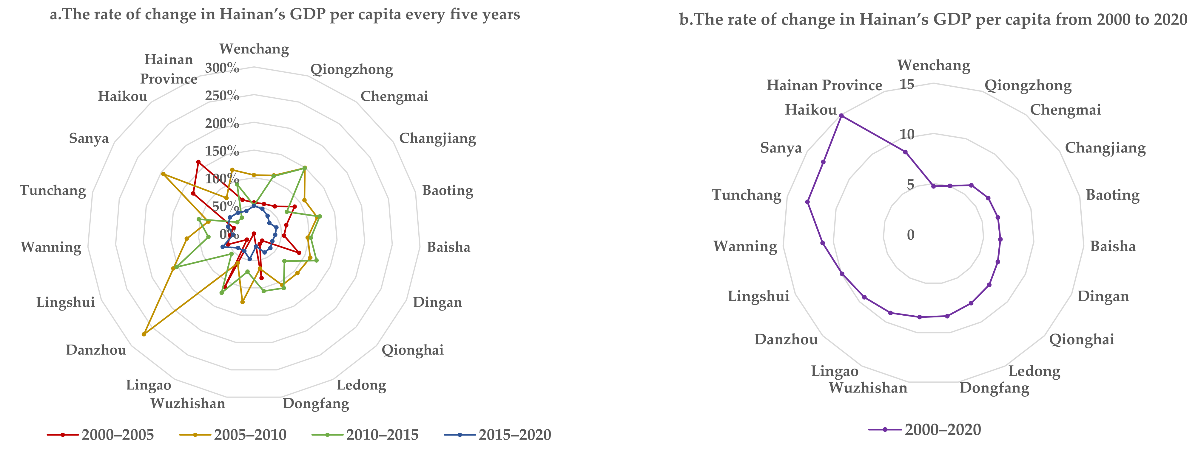
2.1. Study Area

Hainan Province (18.80°–20.10° N, 108.37°–111.03° E) is located at the northern end of the continental shelf of the South China Sea, which has 18 cities and counties and covers an area of approximately 34,000 km². The province’s landforms are diverse. Its topography is high in the middle and low on all sides. The terrain is a peak, with Wuzhishan (1867 m) and Yingge Ling (1811 m) as the core of the uplift. This gradually descends from the middle to the surrounding mountains, hills, platforms and plains (Figure 1). Hainan Province has a typical tropical monsoon maritime climate. It has a hot, rainy climate with long summers and no winter. The annual precipitation of 1000–2500 mm is unevenly distributed between the rainy and dry seasons, and across the province. The average annual temperature is 23.8–26.2 °C. Hainan Province is dry in the west and wet in the east [43,44]. Hainan has witnessed rapid social and economic development, rapid urban expansion and drastic land changes since the construction of Hainan International tourism island in 2009, which have profoundly affected the structure and function of the entire island ecosystem. This profoundly affects the structure and function of the entire province ecosystem. At present, the province’s land use is mainly forest and farmland, which account for nearly 90% of the total area. The province is rich in forest resources and diverse in ecosystems and has the most intact tropical natural forest in the country, which has laid a solid foundation for the development strategy of Hainan’s ecological province and the construction of the national ecological civilization experimental zone.

2.2. Data Sources and Preprocessing

The land use classification data of Hainan Province in 2000, 2005, 2010, 2015 and 2020 came from the Resource Science and Satellite Center (http://www.resdc.cn/, accessed on 31 August 2021), with a spatial resolution of 30 m and a classification accuracy of more than 85% [45]. The Resource Science and Satellite Center’s classification system includes 6 primary classes and 22 subclasses. On this basis, this study established an ecosystem classification system table (

Table 1. Ecosystem classification system.

Ecosystems Classes	LUCC Classes
Primary Classes	Subclasses	Codes
Forest	Forestland	21
	Sparse woods	22
	Other forestland	24
Shrubs	Shrubs	23
Farmland	Paddy field	11
	Dry farmland	12
Grassland	High-covered grassland	31
	Medium-covered grassland	32
	Low-covered grassland	33
River	Rivers and canals	41
Wetlands	Lakes	42
	Reservoir pond	43
	Tidal flat	45
	Beach	46
	Marshland	64
Construction land	Urban residential area	51
	Rural residential area	52
	Other construction land	53
Bare land	Desert sand	61
	Saline-alkali land	63
	Bare land	65
	Bare rock	66

). We divided ecosystems into 8 primary classes: farmland, forest, grassland, shrubs, wetlands, bare land, river, and construction land.

The socioeconomic data such as food crop yield, area and agricultural product prices, agricultural product price index, population, and per capita GDP needed to evaluate the ESV were derived from the “China Statistical Yearbook”, “Hainan Statistical Yearbook”, and “National Agricultural Products” compilations of cost–benefit information and national economy and development reports of various years. The administrative division data and digital elevation model (DEM) data came from the geographic and national conditions monitoring cloud platform (http://www.dsac.cn, accessed on 28 August 2021).

The NPP data were mosaicked by the MODIS satellite MOD17A3HGF.006 in the Google Earth Engine (GEE) platform based on the shapefile data of Hainan Province, with a spatial resolution of 500 m. The NDVI data were calculated by using the annual maximum value synthesis method for Landsat TM/OLI image data after cloud removal on the GEE cloud platform, with a spatial resolution of 30 m.

2.3. Methods

Figure 2 is the flow chart of the calculation and driving force analysis of ESV and EEC in Hainan Province. It mainly includes five steps: (1) Using land use data to classify ecosystem data; the spatial and temporal variation characteristics of ecosystem data were analyzed and the ecosystem service value equivalent per unit area of Hainan Province was constructed based on the ecosystem service value equivalent per unit area of China. (2) Calculating a standard equivalent value and socio-economic adjustment coefficient using social and economic statistics data; the annual NPP and NDVI data were calculated by the GEE platform and administrative division data to improve the biomass factor adjustment factor. (3) Calculating the ESV results of Hainan Province and analyzing the spatiotemporal variation characteristics of ESV. (4) Calculating the economic environment coordination index through the coupling model of ESV per unit area and GDP per capita, and analyzing the spatiotemporal variation characteristics of EEC. (5) Driving factors of ESV and EEC are analyzed by using the GeoDetector model (9 driving factors, such as DEM and cultivated land area).

2.3.1. Ecosystem Category Analysis Method

We used single land use dynamics [46] and comprehensive land use dynamics [47] to analyze the number and degree of ecosystem types and regional differences in ecosystem changes. These results reflected the severity of changes in ecosystem types in the assessment area.

The state of the ecosystem was expressed by the land use intensity (LUI), which reflects the effects of human activities on the natural world [48]. The calculation method is as follows:

$$LUI=\frac{S_{CLE}}{S}\times 100\%$$

(1)

$$S_{CLE}={\displaystyle \sum _{i=1}^n\left(S{L}_i\times E{C}_i\right)}$$

(2)

where $LUI$ is the land use intensity; $S_{CLE}$ is the equivalent area of construction land; $S$ is the total area of the region; $S{L}_i$ is the area of land use/cover type i; $E{C}_i$ is the equivalent conversion coefficient of construction land for land use/cover type i; and n is the land use/cover type in the area.

According to the two-level stepwise algorithm: (1) The first level. We set the eigenvalue of the unchanged surface natural property and unused natural cover as 0, and the eigenvalue of the artificial surface layer and blocked water, nutrient, air and heat exchange above and below the surface as 1. In other words, we used natural cover change and the exchange of water, nutrients, air and heat above and below the surface as indicators, and divided them into 5 equal parts from 0 to 1. (2) The second level. We marked the unchanged surface natural cover being used, the changed natural cover—planting perennial plants, and the changed natural cover—planting 1-year-old crops, and divided them into 3 equal grades from 0 to 0.2. We obtained the conversion coefficient of the construction land equivalent for different land use/cover types according to the two-level stepwise algorithm [48], as shown in

Table 2. Equivalent conversion coefficients of different land use types.

Land Use Type	Equivalent Conversion
Farmland	0.200
Forest	0.067
Shrubs	0.060
Grassland	0.100
Wetlands	0.200
Construction land	1.000
Bare land	0.001
River	0.002

.

2.3.2. Dynamic ESV Evaluation Method

Xie et al. revised the ecosystem service classification and equivalent table according to the specific situation in China [49]. On the basis of Xie et al.’s research, we added the socioeconomic adjustment coefficient and spatial heterogeneity adjustment coefficient [50]. Then, the equivalence factors were matched according to the status of Hainan’s ecosystem. Finally, the Hainan Ecosystem Service Value Equivalent Table of Unit Area was formulated (

Table 3. Ecosystem service value equivalent per unit area of Hainan Province.

Categories	Sub-Categories	Farmland	Forest	Shrubs	Grassland	Wetlands	Bare Land	River	Construction Land	Total
Supplying services	Food production	1.105	0.29	0.19	0.38	0.51	0	0.8	0.01	3.285
	Raw material production	0.245	0.66	0.43	0.56	0.5	0	0.23	0	2.625
	Water supply	−1.305	0.34	0.22	0.31	2.59	0	8.29	−7.51	2.935
Regulating services	Gas regulation	0.89	2.17	1.41	1.97	1.9	0.02	0.77	−2.42	6.71
	Climate regulation	0.465	6.5	4.23	5.21	3.6	0	2.29	0	22.295
	Environment purification	0.135	1.93	1.28	1.72	3.6	0.1	5.55	−2.46	11.855
	Hydrological regulation	1.495	4.74	3.35	3.82	24.23	0.03	102.24	0	139.905
Supporting services	Soil conservation	0.52	2.65	1.72	2.4	2.31	0.02	0.93	0.02	10.57
	Maintenance of nutrient circulation	0.155	0.2	0.13	0.18	0.18	0	0.07	0	0.915
	Biodiversity	0.17	2.41	1.57	2.18	7.87	0.02	2.55	0.34	17.11
Cultural services	Recreation and culture	0.075	1.06	0.69	0.96	4.73	0.01	1.89	0.01	9.425
Total		3.95	22.95	15.22	19.69	52.02	0.2	125.61	−12.01	227.63

).

Specifically, the standard equivalent coefficient is defined as 1/7 of the economic value of farmland’s annual grain. To eliminate the impact caused by price fluctuations over the years, we increased the Consumer Price Index (CPI). We used formula (3) and related statistics to convert all prices based on 2015 prices. According to relevant statistical data, we collected the national average price and national output per unit area of each grain crop in 2000, 2005, 2010, 2015 and 2020. We found that the standard equivalent factor value of Hainan Province in each year was 1223.98 CNY/hm², 1289.59 CNY/hm², 1533.58 CNY/hm², 1627.53 CNY/hm², and 1472.49 CNY/hm², respectively. Finally, the average value of the data in the five periods was 1429.44 CNY/hm², as the standard equivalent factor value.

With the development of the economy, people will pay more attention to protecting ecological systems and the ecological environment, which means that the costs people must pay to protect the ecosystem are becoming increasingly affordable. We adjusted for this by adding the socioeconomic development coefficient [51]. The socioeconomic development coefficient includes the ability to pay represented by GDP, the willingness to pay represented by Engel’s coefficient, and the resource scarcity coefficient represented by population density.

As the ecosystem changes in different years and different regions, the ESV also changes accordingly. Biomass has a great impact on ecosystems and it is positively correlated with ESV. In this paper, annual NPP and annual NDVI were used as biomass adjustment coefficients reflecting natural biomass. We used these data to modify ESV as a coefficient of spatial heterogeneity.

Some studies assert that construction land provides different ESV (such as soil conservation and resource consumption). Therefore, this paper refers to the relevant literature [47,52,53], and we think that construction land contributes to ESV. Table 3 and

Table 4. Ecosystem service value per unit area in Hainan Province (CNY/hm²).

Categories	Sub-Categories	Farmland	Forest	Shrubs	Grassland	Wetlands	Bare Land	River	Construction Land	Total
Supplying services	Food production	1579.53	414.54	271.59	543.19	729.01	0.00	1143.55	14.29	7232.97
	Raw material production	350.21	943.43	614.66	800.49	714.72	0.00	328.77	0.00	4774.33
	Water supply	−1865.42	486.01	314.48	443.13	3702.25	0.00	11,850.06	−10,735.09	1829.68
Regulating services	Gas regulation	1272.20	3101.88	2015.51	2816.00	2715.94	28.59	1100.67	−3459.24	13,022.20
	Climate regulation	664.69	9291.36	6046.53	7447.38	5145.98	0.00	3273.42	0.00	37,494.21
	Environment purification	192.97	2758.82	1829.68	2458.64	5145.98	142.94	7933.39	−3516.42	18,611.31
	Hydrological regulation	2137.01	6775.55	4788.62	5460.46	34,635.33	42.88	146,145.95	0.00	206,411.14
Supporting services	Soil conservation	743.31	3788.02	2458.64	3430.66	3302.01	28.59	1329.38	28.59	18,196.77
	Maintenance of nutrient circulation	221.56	285.89	185.83	257.30	257.30	0.00	100.06	0.00	1772.51
	Biodiversity	243.00	3444.95	2244.22	3116.18	11,249.69	28.59	3645.07	486.01	26,544.70
Cultural services	Recreation and culture	107.21	1515.21	986.31	1372.26	6761.25	14.29	2701.64	14.29	14,394.46
Total		5646.29	32,805.65	21,756.08	28,145.67	74,359.47	285.89	179,551.96	−17,167.57	325,383.43

show the unit area equivalent factor and unit area equivalent value of Hainan Province, respectively. The specific formula for calculating ESV is as follows:

$$y_n=\left\{\begin{array}{l}100,n=2000\\ x_n,n=2001\\ x_n\times y_{n-1}/100,n=2002,2003,\dots \end{array}\right.$$

(3)

$$ESV={\displaystyle \sum VC\times P_j\times A_j\times PI}$$

(4)

$$VC=\frac{1}{7}\times {\displaystyle \sum _{i=1}^n{m}_i{p}_i{q}_i}/M\times \frac{R}{R_0}$$

(5)

$$P_j=\left(\frac{B_j}{\overline{B}}+\frac{N_j}{\overline{N}}\right)/2$$

(6)

$$PI=W_t\times A_t\times S$$

(7)

$$W_t={\left(\frac{2}{1+e^{-\frac{1}{E{n}_r\times \left(1-P_u\right)+E{n}_u\times P_u}+2.5}}\right)}_A/{\left(\frac{2}{1+e^{-\frac{1}{E{n}_r\times \left(1-P_u\right)+E{n}_u\times P_u}+2.5}}\right)}_N$$

(8)

$$A_t=\frac{pGD{P}_A}{pGD{P}_N}\times \frac{U_A}{U_N}$$

(9)

$$S=\ln P_A/\ln P_N$$

(10)

where $x_n$ refers to the CPI in the nth year relative to the previous year = 100; $y_n$ refers to CPI in the nth year relative to the base year 2000 = 100; n = 2000,…,2020; $ESV$ is the total value of ecosystem service functions (CNY); $VC$ is the value coefficient of ecosystem service function (CNY/hm²); $P_j$ is the adjustment coefficient of spatial heterogeneity; $A_j$ is the area of type j ecosystem (hm²); and $PI$ is the social and economic adjustment coefficient. i is the type of grain in Hainan Province, of which the main grain types are rice, soybeans, etc.; n is the number of food categories; $m_i$ is the area of type i grain (hm²); $p_i$ is the national yield per unit area of type i grain (kg/hm²); $q_i$ is the national average price of category i grain (CNY/kg); $M$ is the total area of n kinds of grain (hm²); $R$ is the grain yield per unit area of farmland in Hainan Province (t/hm²); and $R_0$ is the national grain output per unit area of farmland (t/hm²). $B_j$ is the average annual NPP (t/hm²) of ecosystem type j in Hainan Province; $\overline{B}$ is the average annual NPP of this type of ecosystem nationwide (t/hm²); $N_j$ is the average annual NDVI value of the category j ecosystem in Hainan Province; and $\overline{N}$ is the average annual NDVI value of this type of ecosystem across the country. $W_t$ is the willingness to pay; $E{n}_u$ is the urban and rural Engel’s coefficient in year t representing the urban Engel’s coefficient and the rural Engel’s coefficient, respectively; and $P_u$ is the proportion (%) of the urban population in year t. $A_t$ is the ability to pay; $pGD{P}_A$ is the GDP per capita of the study area (CNY); $pGD{P}_N$ is the national GDP per capita (CNY); $U_A$ is the urbanization rate of the study area (%); and $U_N$ is the national urbanization rate (%). $S$ is the resource scarcity index; $P_A$ is the population density of the study area (person/km²); and $P_N$ is the national population density (person/km²).

2.3.3. Calculation Method of EEC

The coordination index can reflect the strength of the interaction between different systems and the degree of coordination. In this paper, the ESV per unit area was used to characterize the ecological environment in different regions [42], and the per capita GDP was used to characterize the level of economic development in different regions [54]. We constructed a coordination index between the ESV and GDP per capita and established different coordination levels [29] (

Table 5. Level of coordination degree between economic development and environmental conditions.

Level	High Maladjustment	Mid Maladjustment	Basic Coordination	Mid Coordination	High Coordination
D	(0,0.2]	(0.2,0.4]	(0.4,0.6]	(0.6,0.8]	(0.8,1]

).

(a)

Data Standardization

To eliminate the influence of different dimensions on the calculation results of the coordination index, this paper used the range method to standardize the ESV per unit area and GDP per capita data in 2000, 2005, 2010, 2015, and 2020 [36], as follows:

$$QESV=\frac{QES{V}_0-QES{V}_{\min }}{QES{V}_{\max }-QES{V}_{\min }}$$

(11)

$$QGDP=\frac{QGD{P}_0-QGD{P}_{\min }}{QGD{P}_{\max }-QGD{P}_{\min }}$$

(12)

where $QESV$ and $QGDP$ are the standardized values of ESV per unit area and GDP per capita; $QESV$ and $QGD{P}_0$ are the original value of ESV per unit area and GDP per capita; $QES{V}_{\max }$ and $QGD{P}_{\max }$ are their maximum values; and $QES{V}_{\min }$ and $QGD{P}_{\min }$ are their minimum values.

(b)

Coordination index

The degree of coordination index can not only reflect the strength of the interaction between economic development and regional environment, but also reflect the degree of coordination between them. This paper constructs the coordination index between ESV and GDP per capita.

$$T=\mathsf{\alpha }\times QESV+\mathsf{\beta }\times QGDP$$

(13)

$$C=\sqrt{\frac{QGDP\times QESV}{{\left(QGDP+QESV/2\right)}^2}}$$

(14)

$$D=\sqrt{T\times C}$$

(15)

where $D$ is the EEC; the larger the value of $D$, the better the EEC in the region. $C$ is the degree of coupling; $T$ is the composite index; $QESV$ and $QGDP$ are the ESV per unit area and GDP per capita, respectively; and $\mathsf{\alpha }$ and $\mathsf{\beta }$ are undetermined weights for the ESV per unit area and GDP per capita, respectively. Economic development is based on environmental quality, and environmental quality is affected by economic development. Therefore, we believe that economic development is as important as the ecological environment ($\mathsf{\alpha }$ = $\mathsf{\beta }$ = 0.5) [29].

2.3.4. Driving Force Analysis Method

To explore the driving factors of ESV (Y1) and EEC (Y2), we chose six socioeconomic and human activity factors: cultivated land area (X1); total population (X2); total real estate investment (X3); total output value of agriculture, forestry and fishery (X4); number of tourists (X5); LUI (X6); and three natural factors: altitude (X7); precipitation (X8); and temperature (X9) based on relevant research and the actual situation in Hainan Province. We used these factors for driving force analysis.

We used Geodetector to analyze the driving forces of ESV and EEC and used the bivariate correlation method to analyze the correlation between each driving force and ESV and EEC. Geodetector is a set of statistical methods to detect spatial differentiation and reveal the driving force behind it [55]. Factor detection in the Geodetector can detect the spatial divergence of variable Y, which is measured by the q value. The calculation method is as follows:

$$q=1-{\displaystyle \sum _{h=1}^L{N}_h{\mathsf{\sigma }}_h^2}/N{\mathsf{\sigma }}_{}^2$$

(16)

where h = 1, …; L is the stratification of variable Y or factor X; $N_h$ and $N$ are the number of units in layer h and the whole area, respectively; and ${\mathsf{\sigma }}_h^2$ and ${\mathsf{\sigma }}_{}^2$ are the variance of the Y value of layer h and the whole area, respectively. The value range of q is [0, 1]. The larger the value of q, the more obvious the spatial divergence of Y.

3. Results

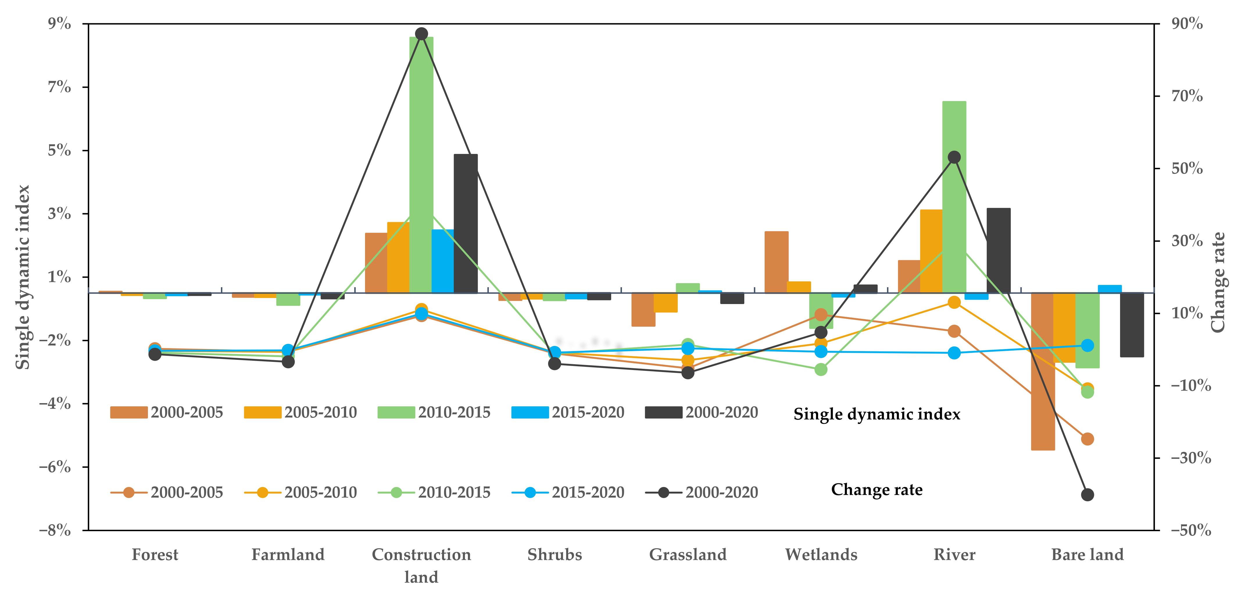
3.1. Ecosystem Category Changes

The spatial distribution of different ecosystems in Hainan Province over the past 20 years is shown in Figure 3a–e. The ecosystem of Hainan Province was dominated by forest, which accounted for more than 55% of the entire province and was mainly distributed in the province’s central and southern regions. Forest was followed by farmland, which accounted for approximately 26% of the entire province and was mainly distributed in the north and around the mountains. The total area of the two ecosystems was close to 82% of the total area of Hainan Province. Other types of ecosystems accounted for a relatively small area. As seen from the spatial distribution, the transformation of Hainan Province’s ecosystem was mainly concentrated in cities, counties, urban areas and coastal areas. Among them, the Haikou, Sanya, Danzhou and Dongfang city urban areas, Yangpu Economic Development Zone, and coastal areas northeast of Wenchang caused major changes in ecosystem types due to urban construction. The main feature of these changes was the conversion of farmland and forest to construction land. The construction of large-scale reservoirs has led to the conversion of farmland, forest, and grassland into wetlands. Second, as a result of Hainan’s afforestation activities on Treasure Island, grassland, farmland and other suitable forestland in Wenchang, Dongfang and other cities and counties were converted into forests in large areas. This somewhat guaranteed the balance of forest resources across the province.

The area classifications and proportions of ecosystems in Hainan Province from 2000 to 2020 are shown in

Table 6. Areas and percentages of different ecosystem classes in Hainan from 2000 to 2020.

Ecosystem Class	2000		2005		2010		2015		2020
	Area (hm2)	Percentage (%)	Area (hm2)	Percentage (%)	Area (hm2)	Percentage (%)	Area (hm2)	Percentage (%)	Area (hm2)	Percentage (%)
Forest	1,929,453	56.38	1,933,173	56.41	1,926,740	56.32	1,910,746	55.86	1,904,057	55.63
Farmland	900,232	26.30	894,627	26.11	888,736	25.98	871,892	25.48	869,676	25.41
Construction land	74,821	2.19	81,821	2.39	90,870	2.66	127,502	3.73	140,128	4.09
Shrubs	252,229	7.37	249,423	7.28	247,214	7.23	244,369	7.14	242,293	7.08
Grassland	123,404	3.61	117,008	3.41	113,545	3.32	115,130	3.37	115,464	3.37
Wetlands	113,959	3.33	124,929	3.65	127,032	3.71	120,021	3.51	119,323	3.49
River	15,593	0.46	16,383	0.48	18,521	0.54	24,105	0.70	23,880	0.70
Bare land	12,788	0.37	9624	0.28	8578	0.25	7569	0.22	7654	0.22

. The single land use dynamics and change rates of each ecosystem during the study period are shown in Figure 4. From 2000 to 2020, only river, wetlands, and construction land were in a state of increase, while the rest of the ecosystem types were in a state of decline. Among them, the area of construction land had the largest increase and increase rate. Its rate of increase reached 87.28%, with an additional area of 65,307 hm². Construction land showed a continuous increasing trend and explosive growth in 2010–2015. The newly increased areas of river and wetlands were 8287 hm² and 5364 hm², with increases of 53.15% and 4.71%, respectively. Forest was the most important type of ecosystem in Hainan Province; it showed a trend of first increasing and then decreasing, reducing its area by 25,396 hm², and its area ratio dropped by 1.32% from 2000 to 2020. Farmland, grassland, shrubs and bare land showed a fluctuating downward trend. Their area reductions were 30,556 hm², 7940 hm², 9936 hm², and 5134 hm², respectively, and their area proportions decreased to 3.85%, 2.58%, 6.43%, 3.94%, and 40.15%, respectively. In terms of area, farmland was the most reduced, followed by forest, shrubs, grasslands and bare land. Bare ground had the largest decline because the area was actively small. In terms of the overall degree of change, construction land had the largest change, followed by bare land. Forest had the smallest change, which meant that forest was the most stable in the ecosystem of Hainan Province.

3.2. Spatial and Temporal Analysis of ESV

As seen in

Table 7. ESV and proportion by ecosystem class in Hainan Province (unit: 10⁶ CNY).

Year	Factor	Forest	Shrubs	Wetlands	Grassland	Farmland	River	Bare Land	Construction Land	Total
2000	ESV	1625.58	124.74	94.22	79.59	122.87	38.31	0.43	−17.32	2068.42
	Percentage	78.59%	6.03%	4.56%	3.85%	5.94%	1.85%	0.02%	−0.84%	100.00%
2005	ESV	1381.84	101.81	87.55	65.41	101.32	34.16	0.37	−16.30	1756.16
	Percentage	78.69%	5.80%	4.99%	3.72%	5.77%	1.94%	0.02%	−0.93%	100.00%
2010	ESV	1378.82	104.17	93.88	65.67	105.68	42.34	0.40	−18.09	1772.87
	Percentage	77.77%	5.88%	5.30%	3.70%	5.96%	2.39%	0.02%	−1.02%	100.00%
2015	ESV	1433.40	107.46	101.35	70.95	109.88	48.64	0.38	−28.06	1843.99
	Percentage	77.73%	5.83%	5.50%	3.85%	5.96%	2.64%	0.02%	−1.52%	100.00%
2020	ESV	1348.13	100.60	98.28	67.29	103.81	46.12	0.36	−29.22	1735.38
	Percentage	77.69%	5.80%	5.66%	3.88%	5.98%	2.66%	0.02%	−1.68%	100.00%

and

Table 8. ESV change rate by ecosystem class from 2000 to 2020 in Hainan Province.

Year	Factor	Forest	Shrubs	Wetlands	Grassland	Farmland	River	Bare Land	Construction Land	Total
2000–2005	Change rate	−14.99%	−18.38%	−7.08%	−17.82%	−17.54%	−10.85%	−14.93%	−5.90%	−15.10%
2005–2010		−0.22%	2.31%	7.23%	0.40%	4.30%	23.97%	9.05%	11.01%	0.95%
2010–2015		3.96%	3.16%	7.95%	8.05%	3.97%	14.87%	−5.64%	55.10%	4.01%
2015–2020		−5.95%	−6.38%	−3.03%	−5.16%	−5.52%	−5.18%	−3.49%	4.14%	−5.89%
2000–2020		−17.07%	−19.35%	4.31%	−15.45%	−15.51%	20.38%	−15.52%	68.72%	−16.10%

, the ESV in Hainan Province showed a trend of first decreasing, then increasing, and then decreasing, and it showed a downward trend as a whole. The ESV dropped from 206.842 billion CNY in 2000 to 175.615 billion CNY in 2005, then increased to 177.286 billion CNY in 2010, increased to 184.399 billion CNY in 2015, and finally decreased to 173.537 billion CNY in 2020. In the past 20 years, the ESV decreased by 33.305 billion CNY, a decrease of 16.1%. The ESV was the highest in 2000, which was mainly due to the biomass adjustment coefficient, the socioeconomic coefficient was the highest (Figure 5), and this year had the least construction land area. In terms of ecosystem types, forest had the highest ESV contribution rate, as high as 77.7%. This was followed by farmland, shrubs, wetlands, grassland, and river; their proportions were 5.9%, 5.8%, 5.3%, 3.8%, and 2.4%, respectively. The ESV contribution rate of bare land was the lowest, at only 0.02%, which showed that the ESV of bare land had the least impact on the overall ESV of Hainan Province. In the past 20 years, only the ESV of wetlands and river showed an upward trend, which was mainly due to the increase in the area of wetlands and river for the construction of reservoirs and fishponds. The ESV of the remaining ecosystems all showed a downward trend. The reason was not only the decline in the area of the remaining ecosystems but also the decline in the biomass adjustment coefficient and the socioeconomic coefficient (Figure 5). Construction land always had a negative effect on the ESV. Although the biomass and socioeconomic regulation factors declined from 2000 to 2020, the ESV of construction land dropped by 68.72%, which showed that the construction land in Hainan Province had increased significantly.

Figure 6 shows the ESV per unit area of different ecosystems. As shown in Figure 6, the river had the highest ESV per unit area, followed by wetlands, forest, grassland, shrubs, farmland and bare land. The ESV per unit area of construction land was always negative. This result shows that to increase the ESV in Hainan Province, we should increase the areas of river, wetlands, and forest to ensure the steady progress of the policy of returning farmland to forest and wetland protection.

Table 9. Proportion of ESV and ESV by different categories of ecosystem services in Hainan Province (unit: 10⁶ CNY).

Year	Categories	Supplying Services			Regulating Services				Supporting Services			Cultural Services
	Sub-Categories	Raw Material Production	Food Production	Water Supply	Climate Regulation	Hydrological Regulation	Gas Regulation	Environment Purification	Soil Conservation	Biodiversity	Maintenance of Nutrient Circulation	Recreation and Culture
2000	ESV	60.32	53.81	−12.61	539.82	508.87	198.93	165.73	232.38	217.76	20.54	82.86
	Percentage	2.92%	2.60%	−0.61%	26.10%	24.60%	9.62%	8.01%	11.23%	10.53%	0.99%	4.01%
2005	ESV	51.10	44.87	−10.33	453.85	436.17	168.19	141.00	197.36	186.22	17.35	70.37
	Percentage	2.91%	2.55%	−0.59%	25.84%	24.84%	9.58%	8.03%	11.24%	10.60%	0.99%	4.01%
2010	ESV	51.41	45.91	−11.47	456.56	447.17	168.65	141.34	198.12	187.33	17.49	70.33
	Percentage	2.90%	2.59%	−0.65%	25.75%	25.22%	9.51%	7.97%	11.18%	10.57%	0.99%	3.97%
2015	ESV	53.70	47.89	−17.87	473.72	471.64	173.96	145.81	206.99	196.52	18.25	73.39
	Percentage	2.91%	2.60%	−0.97%	25.69%	25.58%	9.43%	7.91%	11.22%	10.66%	0.99%	3.98%
2020	ESV	50.57	45.36	−18.98	446.69	445.58	163.19	136.65	194.82	185.33	17.21	68.96
	Percentage	2.91%	2.61%	−1.09%	25.74%	25.68%	9.40%	7.87%	11.23%	10.68%	0.99%	3.97%

and

Table 10. Rate of change in ESV by different categories of ecosystem services in Hainan Province.

Year	Categories	Supplying Services			Regulating Services				Supporting Services			Cultural Services
	Sub-Categories	Raw Material Production	Food Production	Water Supply	Climate Regulation	Hydrological Regulation	Gas Regulation	Environment Purification	Soil Conservation	Biodiversity	Maintenance of Nutrient Circulation	Recreation and Culture
2000–2005	Change rate	−15.27%	−16.62%	−18.1%	−15.93%	−14.29%	−15.45%	−14.92%	−15.07%	−14.49%	−15.57%	−15.08%
2005–2010		0.61%	2.33%	11.04%	0.60%	2.52%	0.28%	0.24%	0.38%	0.60%	0.85%	−0.05%
2010–2015		4.44%	4.31%	55.83%	3.76%	5.47%	3.15%	3.16%	4.48%	4.90%	4.35%	4.35%
2015–2020		−5.82%	−5.29%	6.19%	−5.71%	−5.53%	−6.19%	−6.28%	−5.88%	−5.69%	−5.72%	−6.04%
2000–2020		−16.16%	−15.70%	50.53%	−17.25%	−12.44%	−17.97%	−17.55%	−16.17%	−14.89%	−16.24%	−16.78%

showed the value and change rate of different ecological services from 2000 to 2020. Climate regulation and hydrological regulation were the main functions affecting ecosystem services, and their values accounted for more than 50% of the total value of Hainan Province. The value of maintenance of nutrient circulation and water supply accounted for the smallest proportion. Among these, water supply resources always had a negative impact on the ESV. This was mainly due to the excessive consumption of water resources on construction land and farmland, which showed that water conservation and protection in Hainan Province was urgent. From 2000 to 2020, the value of all individual ecosystem services decreased due to reductions in the biomass adjustment coefficient and socioeconomic adjustment coefficient, and the impact of changes in different ecosystem types. The value of the water supply continuously decreased, mainly because of the rapid expansion of construction land. Although the increase in river and wetlands had a positive effect on the water supply, the increase in the area of the two was much smaller than the increase in construction land, which led to a continuous decrease in the ESV. The reduction in raw material production, hydrological regulation, climate regulation, environmental purification, gas regulation, soil conservation, and recreation and culture was related to the continuous reduction in forest, grassland and shrubs. In terms of the rate of change, the rate in hydrological regulation was the lowest (−12.11%), followed by biodiversity (−15.03%). The change rates of hydrological regulation and biodiversity were lower than those of other ecosystem services mainly due to the increase in the area of wetlands and river, which indicates that the change in ecosystem types had an important impact on the function of ecological services.

As shown in Figure 7, regulation services were the most important function of ecosystem services, with values of up to 68%. Second were support services, the value of which accounted for approximately 23%, and the value of supply services and cultural services accounted for approximately 5% and 4%, respectively. The change trend of the four services during the study period was the same as the total ESV, which showed a trend of first decreasing, then increasing, and then decreasing, and showed a downward trend as a whole.

In summary, the changes in ecosystems and the decline in the biomass adjustment coefficients and socioeconomic adjustment coefficients played important roles in the decline in ESV in Hainan Province. As shown in Figure 5, the biomass adjustment coefficient of Hainan Province dropped from 2.28 to 1.94, a decrease of 14.91% from 2000 to 2020. The advantages of Hainan Province’s NPP and NDVI over China’s average NPP and NDVI continue to decline. The socioeconomic adjustment coefficient dropped from 0.78 to 0.52, a decrease of 33.3%, which showed that the economic development speed of Hainan Province was slower than that of China.

Due to the unit area, the ESV value in some pixels (such as river ecosystem) was much higher than in other pixels. If we used the natural breakpoint method, it may result in poor picture display, while the artificial breakpoint method can control the picture display status and present a better display effect. Therefore, the artificial breakpoint method was used to divide the ESV into six categories, as shown in Figure 8. The ESV of Hainan Province conformed to the spatial distribution characteristics of being high in the middle and low in the surrounding area, which was highly consistent with the spatial distribution of elevation. The reason was the lower LUI in mountainous areas with higher altitudes, which were mainly distributed in forest and grassland ecosystems, and these areas had higher ESV. The surrounding areas with lower elevations had higher LUI, and they were mainly distributed in ecosystems such as construction land and farmland; these areas had lower ESV. The ecosystem with the highest ESV level in Hainan Province was mainly river, which was concentrated in major river areas, with some scattered in the middle. The lowest ESV ecosystem was mainly construction land, which was mainly concentrated in northern Hainan and coastal plains. The high-value areas of ESV in Hainan Province continued to slump and the low-value areas continued to expand from 2000 to 2020.

Figure 9 shows the ESV and ESV per unit area in different periods of cities and counties in Hainan Province. Figure 9b shows that the largest ESV in most cities and counties appeared in 2000, and the lowest ESV occurred in 2020. Among these cities and counties, Qiongzhong’s ESV was always the largest, and Lingao’s ESV was always the lowest. Figure 9b shows a clockwise direction from Lingao to Qiongzhong, and that the overall ESV of each city and county was on the rise. Figure 8a shows that the highest ESV per unit area of most cities and counties occurred in 2000, and the lowest ESV occurred in 2020, which was the same trend as the total ESV. Among these cities and counties, Wuzhishan always had the highest ESV per unit area, and Lingao always had the lowest ESV. Figure 9a shows a clockwise direction from Lingao to Wuzhishan, and the overall ESV per unit area of each city and county showed an upward trend. The ESV per unit area could be used to indicate the regional ecological quality, which showed that the ecological environment of Wuzhishan was the best and that of Lingao was the worst.

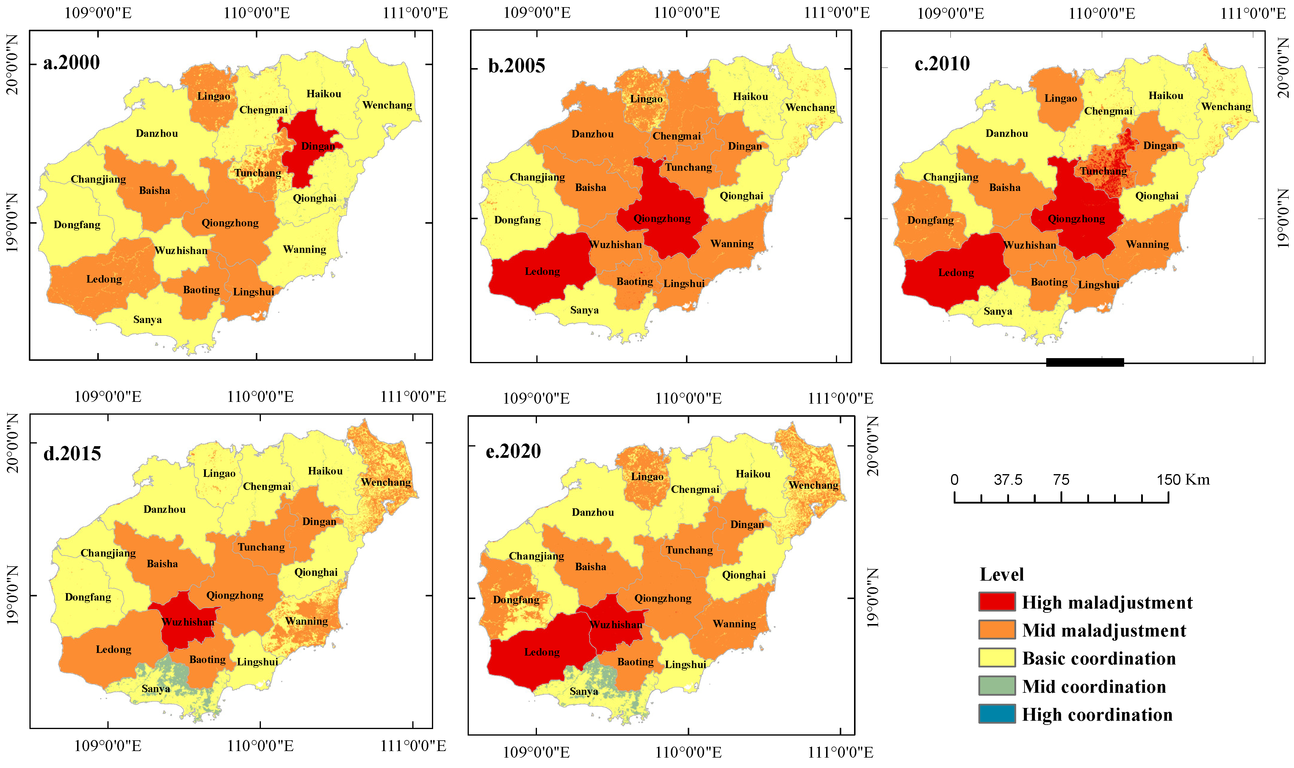
3.3. Changes in the EEC

The GDP of Hainan Province has increased significantly in the past 20 years. It increased from 52.682 billion CNY in 2000 to 553.239 billion CNY in 2020, which was an increase of 10.5 times and represents China’s economic development speed since the beginning of the 21st century. The spatial distribution of GDP per capita is shown in Figure 10. The per capita GDP of Hainan Province changed dramatically in different years and increased rapidly from 2000 to 2020. Spatial distribution was contrary to the spatial distribution of ESV, which showed a distribution pattern of being low in the middle and high in the surrounding areas. Areas with high GDP per capita were mainly distributed in the coastal plains, with Haikou and Sanya having the highest GDP, and the central mountainous areas had low GDP per capita. In 2020, the GDP per capita of Sanya city was 88,900 CNY and that of Ledong County was only 31,000 CNY, which showed that the uneven economic development of Hainan Province was relatively obvious.

The rates of change in GDP per capita in Hainan Province and each city and county are shown in Figure 11. The GDP per capita of Hainan Province rose rapidly. From 2000 to 2020, the province’s average GDP per capita increased by 861%. Haikou, Sanya, Tunchang, and Wanning’s growth rates exceeded 1000%. Wenchang and Qiongzhong had the lowest growth rates, at approximately 500%. The GDP per capita of cities and counties grew the fastest in 2005–2010 and 2010–2015.

The EEC calculation result is shown in Table 10. The overall EEC of Hainan Province declined from 0.42 in 2000 to 0.36 in 2020. It first decreased, then increased, and then decreased, which was consistent with the change trend of the ESV. This was mainly because the GDP per capita was in a state of rapid development, but the decrease in the ESV caused the EEC to show a negative growth trend, and the increase in the ESV caused the EEC to show a positive growth trend. Hainan Province was in a state of basic coordination in only 2000, and it was in a state of mid maladjustment in 2005, 2010, 2015, and 2020.

According to the grading method in Table 5, we divided the EEC into five grades. Therefore, the spatial distribution map of the Hainan EEC was obtained (Figure 12), and the area of each grade was measured (

Table 11. Area statistics of EEC level (km²).

Year	Coordination Level	High Maladjustment	Mid Maladjustment	Basic Coordination	Mid Coordination	High Coordination
2000	Area	1175.43	11,619.16	20,967.4	89.23	1.09
	Percentage	3.472%	34.323%	61.938%	0.264%	0.003%
2005	Area	5414.21	16,236.91	12,139.39	60.28	1.52
	Percentage	15.994%	47.964%	35.860%	0.178%	0.004%
2010	Area	5866.15	13,038.4	14,863.18	83.14	1.45
	Percentage	17.329%	38.516%	43.906%	0.246%	0.004%
2015	Area	1188.39	13,357.01	18,591.9	712.46	2.41
	Percentage	3.511%	39.457%	54.921%	2.105%	0.007%
2020	Area	3895.89	14,133.5	15,181.4	640.2	1.32
	Percentage	11.508%	41.750%	44.846%	1.891%	0.004%

). As seen in the figure, the EEC in the central part of Hainan Province was low in all years. This result was mainly because the GDP per capita in these areas was low but the ESV value was high, so the economic environment development was not coordinated. The EEC was relatively high in the round-island areas, which was mainly because the GDP per capita and ESV in these areas were both high, and the economic and environmental development was more coordinated. In 2000, 2010, 2015, and 2020, Hainan Province had the most land at the basic coordination level. In 2005, Hainan Province had the most land at the mid-maladjustment level. This result was mainly due to the large decline in ESV in 2005 and the rapid growth of GDP per capita. From 2000 to 2020, the change trend of land area in a maladjusted state was the opposite to that of ESV, and the change trend of land area in a coordinated state was the same as that of the ESV. There was very little land with mid and high levels of coordination, scattered around rivers with high ESV values. Since 2015, the area of moderately coordinated land has increased in Sanya, which shows that the EEC of Sanya has improved.

Table 12. Environmental and economic coordination index in Hainan.

Coordination Index	2000	2005	2010	2015	2020
Hainan Province	0.42	0.32	0.35	0.39	0.36
Ledong	0.38	0.12	0.13	0.24	0.11
Wuzhishan	0.47	0.24	0.29	0.01	0.14
Qiongzhong	0.28	0.12	0.17	0.24	0.23
Baisha	0.36	0.28	0.25	0.29	0.24
Tunchang	0.39	0.27	0.20	0.23	0.24
Dingan	0.11	0.24	0.25	0.34	0.30
Baoting	0.30	0.22	0.26	0.35	0.32
Wanning	0.44	0.35	0.37	0.40	0.37
Dongfang	0.46	0.43	0.38	0.45	0.39
Lingao	0.39	0.39	0.34	0.42	0.39
Wenchang	0.49	0.42	0.42	0.40	0.40
Changjiang	0.48	0.45	0.45	0.48	0.45
Qionghai	0.57	0.45	0.45	0.48	0.46
Lingshui	0.33	0.23	0.33	0.45	0.47
Danzhou	0.50	0.36	0.49	0.50	0.48
Chengmai	0.43	0.37	0.42	0.53	0.51
Haikou	0.54	0.56	0.54	0.54	0.53
Sanya	0.50	0.50	0.57	0.58	0.58

shows counties and cities in ascending order of coordination. Sanya’s EEC was the highest in 2015 and 2020, Haikou’s EEC was the highest in 2005 and 2020, and Qionghai’s EEC was the highest in 2000. They were all in a basic coordinated state. Sanya, Haikou, Wenchang, and Changjiang were all in a basically coordinated state over the past 20 years, which showed that the GDP growth of these regions also improved the ESV. Ledong, Qiongzhong, Baisha, Tunchang, Ding’an, and Baoting were all in a state of imbalance in the past 20 years due to the low GDP per capita and high ESV in these areas, so it was necessary to vigorously increase the speed of economic development.

3.4. Analysis of the Driving Force of the Coordination between ESV and EEC

The correlation coefficients between ESV and EEC and each driving force factor are shown in

Table 13. Correlation analysis of 9 driving forces of EEC and ESV.

Index		X1	X2	X3	X4	X5	X6	X7	X8	X9
Y1	Correlation	−0.300	−0.253	−0.203	−0.278	−0.095	−0.821	0.610	−0.010	0.032
	p value	0.000	0.000	0.000	0.000	0.000	0.000	0.000	0.000	0.000
Y2	Correlation	0.499	0.666	0.726	0.579	0.581	0.150	−0.452	−0.079	0.030
	p value	0.000	0.000	0.000	0.000	0.000	0.000	0.000	0.000	0.000

. The p value of each driving force factor was 0.000, which indicated that the results passed the hypothesis test with a significance level of 0.05. The ESV was negatively correlated with X1, X2, X3, X4, X5, X6 and X8. Among them, the ESV had the greatest correlation with LUI, with a value of −0.821. The ESV was positively correlated with X7 and X9. Among them, the ESV was highly correlated with X7, with was 0.61. This result showed that the ESV had a negative correlation with the impact of human activities. The ESV was lower in areas with more severe human activities, while it was higher in biomass-rich areas such as the mountainous areas of Hainan Province. The EEC was positively correlated with X1, X2, X3, X4, X5, X6 and X9. Among them, the EEC had a high correlation with socioeconomic factors and had a negative correlation with X7 and X8. The driving forces of EEC and ESV had opposite effects, which showed that the EEC was higher in the economically developed areas of Hainan Province.

The ESV and EEC driving force results obtained by using the Geodetector are shown in

Table 14. Driving force spatial differentiation.

Index		X1	X2	X3	X4	X5	X6	X7	X8	X9
Y1	q statistic	0.137	0.159	0.087	0.231	0.093	0.712	0.411	0.057	0.056
	p value	0.000	0.000	0.000	0.000	0.000	0.000	0.000	0.000	0.000
Y2	q statistic	0.573	0.635	0.679	0.561	0.555	0.057	0.328	0.194	0.074
	p value	0.000	0.000	0.000	0.000	0.000	0.000	0.000	0.000	0.000

. The p value of each driving force factor was 0.000, which showed that the results passed the hypothesis test with a significance level of 0.05. Among the driving force factors of ESV, the contribution rate of X6 was the highest, with a value of 0.712. Next, X7 had a contribution rate of 0.411. X4, X2 and X1 had contribution rates of 0.231, 0.159 and 0.137, respectively. The contribution rates of the remaining driving force factors were all below 0.1, and the contribution rates of X8 and X9 were the lowest. The ESV was mainly affected by human activity factors and natural factors, and socioeconomic factors had little influence. Among the driving force factors of the EEC, X3 had the highest contribution rate, with a value of 0.679. It was followed by the contribution rates of X2, X1, X4 and X5, which had values of 0.635, 0.573, 0.561, and 0.555, respectively. X7 and X8 had contribution rates of 0.328 and 0.194, respectively. The contribution rate of X6 was the lowest. The EEC was mainly affected by socioeconomic factors, and the contribution rate of each socioeconomic driving force was above 0.55. The EEC was less affected by natural factors.

4. Discussion

4.1. Improvement of Dynamic ESV Assessment Method

ESV assessments have been widely used. However, most studies have not considered the spatial heterogeneity of ESV [30,45,56,57]. In addition, the monetary estimation of ESV is affected by different factors, including resource scarcity, ability to pay, willingness to pay, market price and inflation [58], which will greatly affect the accuracy of the results. This paper comprehensively considered the social and economic development status and regional differences. We used biomass adjustment coefficients, socioeconomic adjustment coefficients and resource scarcity adjustment coefficients to modify the value of the equivalent factor and obtained accurate ESV assessment results. This method allowed us to better explore the degree of EEC in Hainan Province and understand the driving forces that affect ESV and EEC. The monetization of ecosystem services can enable people to better understand the important contribution of ecosystem services to society [5]. The ESV is beneficial to society as a whole, but it is not owned by individuals [59].

We used the biomass adjustment coefficient for the ESV spatial heterogeneity adjustment, and NPP was used to express the area’s net primary production capacity. Hainan Province is at the forefront of the country in terms of ecological quality and it is rich in biological resources [60]. In addition, the equivalent factor of Xie et al. was based on the national level, and biological resources in northwestern China are very scarce [6]. Thus, the ratio of Hainan’s NPP to the national NPP is very large. As an index to evaluate vegetation status, the NDVI can reflect the regional biomass status. To more accurately reflect the biomass ratio between Hainan Province and the country, we used the ratio of the average value of Hainan Province’s NDVI and NPP to the national average value of the NDVI and NPP as the biomass adjustment coefficient to obtain a more accurate spatial heterogeneity distribution situation.

4.2. Ecosystem Changes

As this paper differentiated shrub ecosystem from forest ecosystem, the proportion of forest area is different from the proportion of forest in other studies, which accounts for more than 62% [61]. This study found that the ecosystem of Hainan Province was dominated by forest and farmland. From 2000 to 2020, the structure of the ecosystems was relatively stable, and its overall change was small, with a comprehensive rate of change of approximately 3.22%. Among the ecosystems, the area of construction land and river increased significantly, from 74,821 hm² to 140,128 hm² and 15,593 hm² to 23,880 hm², respectively. The 20-year rates of change were 87.28% and 53.15%, respectively. Due to the promotion of policies such as Hainan International Tourism Island, urban construction and land development further expanded from 2010 to 2015. The growth rate of construction land was the fastest in the past five years. The extensive development model was the main reason for the significant differences in the urbanization level among various regions in Hainan Province. Therefore, we recommend that the government further optimize the allocation of land resources and appropriately limit the expansion of urban construction land. We should rationally lay out the space, structure and scale of industry and urban development in accordance with the requirements of high-quality development and scientifically plan and improve the matching degree with various resources. In addition, we need to further optimize the urban spatial structure.

The higher productivity of aquaculture fishponds [62] and the construction of large reservoirs led to an increase in the wetland area, with a 20-year change rate of 4.71%. The remaining ecosystems all showed a decreasing trend. In the past 20 years, the ecosystem of Hainan Province was mainly transformed from farmland, forest, and wetlands, with contribution rates of 29.82%, 27.07%, and 8.18%, respectively. The transformed ecosystems were mainly construction land and wetlands, with contribution rates of 33.49% and 12.18%, respectively. Among them, the transfer-out and transfer-in ratios of wetlands were relatively large. The reason was that natural wetlands were constantly decreasing, while artificial wetlands such as fishponds were constantly increasing [63,64]. Ecosystem transformation was mainly manifested in the conversion of farmland, forest, and shrubs into construction land. In the past 20 years, their contribution rate was 64.51%, which showed that the rapid expansion of construction land had become the main factor in the loss of farmland and forest [56,65,66]. Construction land was mainly transferred out of farmland, which was similar to the results of previous studies [31,65,67]. This resulted in the reduction of a large amount of high-quality farmland and increased the fragmentation of farmland, leading to prominent food security problems [68]. There was also the conversion of wetlands to farmland and the conversion of natural wetlands to constructed wetlands. This was because although the overall area of wetlands has shown an increasing trend, the artificial wetlands in Hainan Province were expanding rapidly, and reclamation and breeding and port development [63] had severely damaged the natural wetland resources in Hainan Province. Therefore, natural wetlands urgently need to be protected.

4.3. ESV Status and Changes

Studies have shown that the ESV of Hainan Province dropped from 206.842 billion CNY in 2000 to 173.537 billion CNY in 2020 (Table 7), and the overall ESV biology has shown a downward trend, which is very consistent with the results of Sui et al. and Sun et al. [43,69]. Ecosystem changes and a decline in biomass adjustment coefficients and socioeconomic adjustment coefficients played important roles in the decline in ESV in Hainan Province.

As the dominant category of Hainan Province, forest ecosystem had the highest contribution rate to ESV, accounting for 78%. Forest’s ESV was higher due to not only its larger area but also its higher ESV per unit area. It was the most important ecosystem category in Hainan Province, which is very consistent with the results of Deng et al. [70]. Rivers and wetlands had the highest ESV per unit area, which is very consistent with the results of Xie et al., Hasan et al., etc. [6,20,42,56,67,71]. However, their contribution rates to ESV were low, because the river and wetland areas of Hainan Province are small. Therefore, policies such as increasing river and wetland areas, returning farmland to wetland, and returning farmland to forest are important means to improve ESV [72]. The ESV of construction land had a negative value, and the rapid expansion of construction land in the past 20 years has provided increasingly negative values. Wuzhishan, Qiongzhong, Baisha and other places had relatively large areas of forest and wetlands, and the area of construction land was relatively small, so the unit ESV in these areas was relatively high (Figure 8). Many studies regard construction land as worthless in terms of research [49,73]. Some studies have also shown that construction land can provide some ecosystem services, such as culture and entertainment [53]. However, the ecological harm it brings will exceed the ecological benefits [52], which will cause the ecological environment to be destroyed, so we agree that construction land provides a negative value.

The first-level category of ecosystem services (Figure 6) showed that regulation services were the most important function, with the ESV accounting for up to 68%, followed by support services, with the ESV accounting for approximately 23% and cultural services accounting for the least, at approximately 4%, which is highly similar to many studies [58]. The secondary classification showed that climate regulation, hydrological regulation, soil conservation and biodiversity were the main ecological service functions of Hainan Province. Among them, water supply provided a negative value. The reason was that the high level of water consumption of construction land and farmland exceeded the water supply service of the ecosystem. Although Hainan Province is located on the equator and has plenty of rainfall, there is a significant engineering water shortage due to the large slope of the province area and the difficulty of storing freshwater resources [74]. Therefore, the problem of water shortages in Hainan urgently needs to be addressed.

4.4. EEC Status and Changes

Studies have shown that Hainan’s GDP grew rapidly, increasing by 550.557 billion CNY. Its ESV dropped by 33.305 billion CNY, and the growth rate of ESV was lower than that of GDP from 2000 to 2020 [29]. The EEC declined from 0.42 to 0.36 and degraded from the basic coordinated state to the mid-maladjusted state. This result shows that the economic development of Hainan Province and the protection of its ecosystem were not well coordinated, and it was necessary to rationally allocate land resources and the development of the ecological economy. The change trends of EEC and ESV were consistent. The reason was that GDP per capita was in a state of rapid development, but the decline in ESV caused the EEC to show a negative growth trend. The economic development of Hainan Province was unevenly distributed on the province. The GDP per capita of the eastern, western and central parts of Hainan Province showed a stepwise downward trend (Figure 9). The distribution of the ESV was also uneven (Figure 7). The ESV was higher in the central region and lower in the east and west. These caused the uneven distribution of the EEC in Hainan Province. As Hainan Province led the country in ecological quality and its environment was relatively good, the ecological economy was a prominent shortcoming in the construction of Hainan’s ecological civilization [75]. Therefore, the conclusion of this study is different from the literature, which believes that the low degree of economic environment coordination is due to the better regional economic development and the poorer environment [29,30]. As a key ecological protection area, Hainan was subject to multiple protections at the national and provincial levels [76]. We thought that the reason for the low degree of EEC in the central region of Hainan Province was that its environmental condition was good but the economic level was too low, and the economic level could not keep up with the environmental conditions. The reason for the higher degree of EEC in the eastern and western regions of Hainan was that these regions had higher economic levels, which could be coordinated with good environmental conditions. Therefore, the improvement of EEC in Hainan Province requires not only the rational allocation of land resources and the protection of forest, wetlands, and other ecosystems but also the vigorous development of ecological economy, considering the organic integration of economic construction and the various ecological elements of mountains, water, farmland, forest, lakes and grasses. Hainan should develop a characteristic ecological economy while protecting the ecology so that the economy and the environment can develop in harmony.

4.5. Drivers of ESV and EEC

Studies have shown that LUI was the most important factor affecting ESV. The LUI in Geodetector contributed the most to the ESV, with a value of 0.712 (Table 14). LUI was related to human activities and was the highest for construction land and farmland, which is highly similar to Xu et al. [48]. There was a significant negative correlation between LUI and ESV, which indicated that the expansion of construction land was an important factor in the reduction of ESV. These results are highly consistent with previous studies [43,47,56,57,58,67]. The ESV had a significant positive correlation with the DEM, which was affected by the distribution characteristics of Hainan’s landforms. The high-altitude mountainous areas in the central part were mainly distributed in forest, wetlands, and other ecosystems with low LUI, so the ESV in these areas was high. The low-altitude coastal plains were mainly distributed in ecosystems with high LUI, such as farmland and construction land, so the ESV of these areas was low. The selected social and economic factors, such as cultivated land area and total real estate investment, had a low contribution rate to ESV. They were mostly negatively correlated with ESV. This result shows that social and economic development, such as urban expansion, population growth, and real estate development, will cause a certain degree of deterioration in ESV, which is very consistent with the results of Zhang et al., Lei et al., etc. [43,45,77]. Therefore, we need to control the intensity of land use and rationally allocate land resources to strengthen sustainable land use to improve Hainan’s ESV.

The driving factor that had the greatest impact on EEC was the total real estate investment, with a value of 0.679 (Table 14). In addition, socioeconomic factors such as cultivated land area and number of tourists all had a greater impact on EEC, with values above 0.55. All socioeconomic factors and EEC were positively correlated, while natural factors such as the DEM were negatively correlated with low contribution rates. This result shows that Hainan Province’s EEC was better in areas where people’s living standards were higher due to the better overall environmental quality. The areas with the best EEC in Hainan were the places with the best development of ecotourism. Therefore, to improve the EEC of Hainan Province, it is necessary to vigorously develop ecotourism and other characteristic economic industries to maintain the rapid growth of people’s income while not damaging the environment.

4.6. Policy Suggestion

To improve the EEC of Hainan Province, the ESV status has also been steadily improved. Therefore, the relationship between development and protection should be handled well in the process of regional land development and utilization. We recommend that the government draft and implement strict and effective policies to control the erosion of land from construction land to natural ecosystems. In addition, the government should rationally plan the spatial distribution of urban space, agricultural space and ecological space [78]. For example, the government should: (1) strengthen the planning of green space systems to increase the value of urban ecosystem services; (2) build multiple green space ecosystems, including parks, nurseries, and shelterbelts, and build artificial lakes, wetlands, forest parks, suburban water conservation forests, forests around the city, and large areas of lawn to reduce the impact of urban expansion on ecosystem services; (3) strictly implement the overall spatial planning of “multiple regulations in one” and the red line management of marine and land ecological protection in Hainan Province and implement the land management policy based on maps; and (4) pay attention to the protection and restoration of high-ESV areas such as wetlands, river and forest; maintain and strengthen the continuity and integrity of the entire province ecosystem; and guide land use to develop in the direction of ESV preservation or appreciation.

In addition, Hainan Province must adhere to the principle of “ecology first, green development” to achieve the coordinated development of its economic environment [71]. Hainan Province must speed up the adjustment of its economic structure, promote industrial transformation and upgrading, guide the rationalization of the spatial layout of industrial functions, and promote green and high-quality development. First, local governments must adhere to the equal emphasis on environmental protection and economic growth and regard strengthening ecological protection as an important means to adjust economic structure, transform economic growth patterns, and seek development in environmental protection [79]. Second, they must change their agricultural production method from a single water-intensive agricultural planting method to a diversified modern agricultural model that consumes less water, such as ecological agriculture and sightseeing agriculture, to dramatically curb the large-scale consumption of agricultural water. The government should vigorously promote a reduction in the use of fertilizers and pesticides, continuously strengthen the utilization of agricultural waste resources and the improvement and utilization of arable land, and actively build an agricultural brand of ecological recycling. Third, the ecological economy must be vigorously developed. We must firmly grasp the huge advantages of Hainan Province’s high ecological quality and the construction of a free trade province. It is necessary to lead comprehensive efforts in resources, environment, ecology, growth quality, production methods, lifestyles, and social development to focus on the transformation of social development, production methods and lifestyles, in order to achieve coordinated economic and environmental development. The government should give full play to the unique advantages of vacation tourism; make full use of ethnic villages, ancient towns, historic sites, natural landscapes and other resources; and adjust production, living and ecological space in a reasonable way according to its own natural landscape, regional characteristics, cultural traditions, ethnic characteristics and industrial planning. We will promote the organic integration of urban and rural construction with investment attraction, industrial development, tourism and vacation, health and medical care, cultural cultivation and ecological protection; turn Hainan’s tourism industry into the most competitive industry with the greatest potential; and build a green ecological urban and rural area that is livable and suitable for working, traveling and nourishing. Fourth, the government must promote the construction of an ecological civilization, strengthen education on ecological civilization, raise awareness of ecological protection and cultivate a low-carbon and green lifestyle for the whole people.

5. Conclusions

This paper used NDVI and NPP data to improve the biomass adjustment factor, and used the ability to pay, willingness to pay, and resource scarcity to construct the socio-economic adjustment factor based on the benefit transfer method and LUCC data of Hainan Province. We measured the temporal and spatial characteristics of Hainan’s dynamic ESV from 2000 to 2020. This article proposed a new coupling model of economic and environmental conditions. We used unit ESV as an environmental factor and GDP per capita as an economic factor. Then, we used the coupling analysis method to measure the EEC of Hainan Province. Finally, a detailed analysis of the driving force factors of the ESV and EEC was carried out. A powerful exploration of the assessment of the coordination of ESV and economic and environmental development in regional areas has been realized.

The results show that Hainan Province has the largest forest area and the least bare land area. The area of forests, farmland and grassland continued to decrease from 2000 to 2020. These ecosystems had positive values of ESV. Forests provided the highest ESV (above 77%), and rivers had the highest unit ESV (above 200,000 CNY/ha). Construction land was increasing rapidly, but it had a negative ESV value. Moreover, the advantages of Hainan Province’s NPP and NDVI relative to the national average of NPP and NDVI continued to decline, and the economic development speed of Hainan Province slowed down relative to the economic development speed of the whole country. All these factors led to a decline in the ESV of the ecosystem, reduced to 33.305 billion CNY. The overall EEC of Hainan Province dropped by 0.06, and the state of EEC dropped from basic coordination to a moderately unbalanced state due to the good environmental quality and the slowdown in economic growth. In terms of driving force analysis, the LUI was the most important factor affecting ESV, with a value of 0.712. Socioeconomic factors and human activities were negatively correlated with ESV. The total real estate investment was the most important factor affecting the EEC, with a value of 0.679. Socioeconomic factors and human activities had a significant positive correlation with the EEC. The spatial distributions of GDP per capita and EEC were opposite to the spatial distribution of ESV. This result shows that economic growth will reduce ESV, but the reason for the EEC in Hainan Province was that the ecological economy was low and the ecological quality was high. Therefore, we must pay more attention to the coordination of economic development and ecological protection to seek green development in future land use planning and social and economic development.

There are still some shortcomings in this study, such as the spatial resolution of LUCC data and NPP data, the amount of GDP data not being very high, and the accuracy of ESV not being evaluated, etc. Therefore, in future research, we consider using high-resolution remote sensing data such as Sentinel satellites to interpret land use types; using the CASA model or downscaling models to obtain higher-resolution NPP data; adding soil conservation inverted by the RUSLE model data and precipitation data to improve spatial heterogeneity adjustment factors; further obtaining township-level GDP data; exploring the appropriate method to evaluate the accuracy of ESV results; using the Invest model to calculate ESV, and using this ESV to calculate the township-scale economic and environmental coordination; and exploring more effective methods to put forward more scientific and reasonable suggestions for the coordinated development of the economic environment.

References

1. Assessment, M.E. Ecosystems and Human Well-Being; Island Press: Washington, DC, USA, 2005; Volume 5, p. 563. [Google Scholar]
2. Kubiszewski, I.; Costanza, R.; Anderson, S.; Sutton, P. The future value of ecosystem services: Global scenarios and national implications. In Environmental Assessments; Edward Elgar Publishing: Northampton, MA, USA, 2020. [Google Scholar]
3. Costanza, R.; d’Arge, R.; De Groot, R.; Farber, S.; Grasso, M.; Hannon, B.; Limburg, K.; Naeem, S.; O’neill, R.V.; Paruelo, J. The value of the world’s ecosystem services and natural capital. Nature 1997, 387, 253–260. [Google Scholar] [CrossRef]
4. Xie, G.; Lu, C.-X.; Cheng, S. Progress in evaluating the global ecosystem services. Resour. Sci. 2001, 23, 5–9. [Google Scholar]
5. Costanza, R.; De Groot, R.; Sutton, P.; Van der Ploeg, S.; Anderson, S.J.; Kubiszewski, I.; Farber, S.; Turner, R.K. Changes in the global value of ecosystem services. Glob. Environ. Change 2014, 26, 152–158. [Google Scholar] [CrossRef]
6. Xie, G.; Zhang, C.; Zhang, L.; Chen, W.; Li, S. Improvement of the evaluation method for ecosystem service value based on per unit area. J. Nat. Resour. 2015, 30, 1243. [Google Scholar]
7. Xie, G.; Zhen, L.; Lu, C.-X.; Xiao, Y.; Chen, C. Expert knowledge based valuation method of ecosystem services in China. J. Nat. Resour. 2008, 23, 911–919. [Google Scholar]
8. Pickard, B.R.; Van Berkel, D.; Petrasova, A.; Meentemeyer, R.K. Forecasts of urbanization scenarios reveal trade-offs between landscape change and ecosystem services. Landsc. Ecol. 2017, 32, 617–634. [Google Scholar] [CrossRef]
9. Zhou, J.; Wu, J.; Gong, Y. Valuing wetland ecosystem services based on benefit transfer: A meta-analysis of China wetland studies. J. Clean. Prod. 2020, 276, 122988. [Google Scholar] [CrossRef]
10. Song, W.; Deng, X. Land-use/land-cover change and ecosystem service provision in China. Sci. Total Environ. 2017, 576, 705–719. [Google Scholar] [CrossRef] [PubMed]
11. Zhongyuan, Y.; Hua, B. The key problems and future direction of ecosystem services research. Energy Procedia 2011, 5, 64–68. [Google Scholar] [CrossRef] [Green Version]
12. Jian, S. Research advances and trends in ecosystem services and evaluation in China. Procedia Environ. Sci. 2011, 10, 1791–1796. [Google Scholar] [CrossRef] [Green Version]
13. Zhang, Y.; Liu, Y.; Zhang, Y.; Liu, Y.; Zhang, G.; Chen, Y. On the spatial relationship between ecosystem services and urbanization: A case study in Wuhan, China. Sci. Total Environ. 2018, 637, 780–790. [Google Scholar] [CrossRef] [PubMed]
14. Ouyang, Z.; Zheng, H.; Xiao, Y.; Polasky, S.; Liu, J.; Xu, W.; Wang, Q.; Zhang, L.; Xiao, Y.; Rao, E. Improvements in ecosystem services from investments in natural capital. Science 2016, 352, 1455–1459. [Google Scholar] [CrossRef] [PubMed]
15. Capriolo, A.; Boschetto, R.; Mascolo, R.; Balbi, S.; Villa, F. Biophysical and economic assessment of four ecosystem services for natural capital accounting in Italy. Ecosyst. Serv. 2020, 46, 101207. [Google Scholar] [CrossRef]
16. Reining, C.E.; Lemieux, C.J.; Doherty, S.T. Linking restorative human health outcomes to protected area ecosystem diversity and integrity. J. Environ. Plan. Manag. 2021, 64, 2300–2325. [Google Scholar] [CrossRef]
17. Lei, J.; Wang, S.; Wang, J.; Wu, S.; You, X.; Wu, J.; Cui, P.; Ding, H. Effects of Land-Use Change on Ecosystem Services Value of Xunwu County. Acta Ecol. 2019, 39, 3089–3099. [Google Scholar]
18. Yan, F.; Zhang, S.; Su, F. Variations in ecosystem services in response to paddy expansion in the Sanjiang Plain, Northeast China. Int. J. Agric. Sustain. 2019, 17, 158–171. [Google Scholar]
19. Fei, L.; Shuwen, Z.; Jiuchun, Y.; Kun, B.; Qing, W.; Junmei, T.; Liping, C. The effects of population density changes on ecosystem services value: A case study in Western Jilin, China. Ecol. Indic. 2016, 61, 328–337. [Google Scholar] [CrossRef]
20. Hasan, S.; Shi, W.; Zhu, X. Impact of land use land cover changes on ecosystem service value—A case study of Guangdong, Hong Kong, and Macao in South China. PLoS ONE 2020, 15, e0231259. [Google Scholar] [CrossRef] [Green Version]
21. Wang, Z.; Wang, Z.; Zhang, B.; Lu, C.; Ren, C. Impact of land use/land cover changes on ecosystem services in the Nenjiang River Basin, Northeast China. Ecol. Processes 2015, 4, 11. [Google Scholar] [CrossRef] [Green Version]
22. Shifaw, E.; Sha, J.; Li, X.; Bao, Z.; Zhou, Z. An insight into land-cover changes and their impacts on ecosystem services before and after the implementation of a comprehensive experimental zone plan in Pingtan island, China. Land Use Policy 2019, 82, 631–642. [Google Scholar]
23. Lei, J.; Chen, Z.; Wu, T.; Li, X.; Yang, Q.; Chen, X. Spatial autocorrelation pattern analysis of land use and the value of ecosystem services in northeast Hainan island. Acta Ecol. Sin. 2019, 39, 2366–2377. [Google Scholar]
24. Yao, X.; Zhou, H.; Zhang, A.; Li, A. Regional energy efficiency, carbon emission performance and technology gaps in China: A meta-frontier non-radial directional distance function analysis. Energy Policy 2015, 84, 142–154. [Google Scholar] [CrossRef]
25. Wang, H.; Zhou, S.; Li, X.; Liu, H.; Chi, D.; Xu, K. The influence of climate change and human activities on ecosystem service value. Ecol. Eng. 2016, 87, 224–239. [Google Scholar] [CrossRef]
26. Chan, K.M.A.; Shaw, M.R.; Cameron, D.R.; Underwood, E.C.; Daily, G.C. Conservation planning for ecosystem services. PLoS Biol. 2006, 4, e379. [Google Scholar] [CrossRef] [Green Version]
27. Rodríguez, J.P.; Beard, T.D., Jr.; Bennett, E.M.; Cumming, G.S.; Cork, S.J.; Agard, J.; Dobson, A.P.; Peterson, G.D. Trade-offs across space, time, and ecosystem services. Ecol. Soc. 2006, 11, 1. [Google Scholar] [CrossRef] [Green Version]
28. Rozelle, S.; Huang, J.; Zhang, L. Poverty, population and environmental degradation in China. Food Policy 1997, 22, 229–251. [Google Scholar] [CrossRef]
29. Zhu, Y.; Yao, S. The coordinated development of environment and economy based on the change of ecosystem service value in Shaanxi province. Acta Ecol. Sin. 2021, 41, 3331–3342. [Google Scholar]
30. Chen, W.; Zeng, J.; Zhong, M.; Pan, S. Coupling Analysis of Ecosystem Services Value and Economic Development in the Yangtze River Economic Belt: A Case Study in Hunan Province, China. Remote Sens. 2021, 13, 1552. [Google Scholar] [CrossRef]
31. Xu, Q.; Yang, R.; Zhuang, D.; Lu, Z. Spatial gradient differences of ecosystem services supply and demand in the Pearl River Delta region. J. Clean. Prod. 2021, 279, 123849. [Google Scholar] [CrossRef]
32. Braat, L.C.; De Groot, R. The ecosystem services agenda: Bridging the worlds of natural science and economics, conservation and development, and public and private policy. Ecosyst. Serv. 2012, 1, 4–15. [Google Scholar] [CrossRef] [Green Version]
33. Li, G.; Fang, C. Global mapping and estimation of ecosystem services values and gross domestic product: A spatially explicit integration of national ‘green GDP’accounting. Ecol. Indic. 2014, 46, 293–314. [Google Scholar] [CrossRef]
34. Zhang, K.-M.; Wen, Z.-G. Review and challenges of policies of environmental protection and sustainable development in China. J. Environ. Manag. 2008, 88, 1249–1261. [Google Scholar] [CrossRef] [PubMed]
35. Wei, W.; Shi, P.; Wei, X.; Zhou, J.; Xie, B. Evaluation of the coordinated development of economy and eco-environmental systems and spatial evolution in China. Acta Ecol. Sin. 2018, 38, 2636–2648. [Google Scholar]
36. Ma, L.; Jin, F.; Song, Z.; Liu, Y. Spatial coupling analysis of regional economic development and environmental pollution in China. J. Geogr. Sci. 2013, 23, 525–537. [Google Scholar] [CrossRef]
37. Gu, K.; Liu, J.; Chen, X.; Peng, X. Dynamic Analysis of Ecological Carrying Capacity of a Mining City. J. Nat. Resour. 2008, 23, 841–848. [Google Scholar]
38. Su, H.; Zhang, Z.; Zhang, X.; Wang, J. Energy analysis on sustainable development of ecological economic system in Shanxi Province. Southwest China J. Agric. Sci. 2019, 32, 1187–1193. [Google Scholar]
39. Wang, Z.; Fang, C.; Wang, J. Evaluation on the coordination of ecological and economic systems and associated spatial evolution patterns in the rapid urbanized Yangtze Delta Region since 1991. Acta Geogr. Sin. 2011, 66, 1657–1668. [Google Scholar]
40. Oliveira, C.; Antunes, C.H. A multi-objective multi-sectoral economy–energy–environment model: Application to Portugal. Energy 2011, 36, 2856–2866. [Google Scholar] [CrossRef]
41. Stern, D.I.; Common, M.S.; Barbier, E.B. Economic growth and environmental degradation: The environmental Kuznets curve and sustainable development. World Dev. 1996, 24, 1151–1160. [Google Scholar] [CrossRef]
42. Zhen, L.; Jinghu, P.; Yanxing, H. The spatio-temporal variation of ecological property value and eco-economic harmony in Gansu Province. J. Nat. Resour. 2017, 32, 64–75. [Google Scholar]
43. Sun, R.; Wu, Z.; Chen, B.; Yang, C.; Qi, D.; Lan, G.; Fraedrich, K. Effects of land-use change on eco-environmental quality in Hainan Island, China. Ecol. Indic. 2020, 109, 105777. [Google Scholar] [CrossRef]
44. Zhou, L.; Gao, S.; Yang, Y.; Zhao, Y.; Han, Z.; Li, G.; Jia, P.; Yin, Y. Typhoon events recorded in coastal lagoon deposits, southeastern Hainan Island. Acta Oceanol. Sin. 2017, 36, 37–45. [Google Scholar] [CrossRef]
45. Zhang, Z.; Xia, F.; Yang, D.; Huo, J.; Wang, G.; Chen, H. Spatiotemporal characteristics in ecosystem service value and its interaction with human activities in Xinjiang, China. Ecol. Indic. 2020, 110, 105826. [Google Scholar] [CrossRef]
46. Redo, D.J.; Aide, T.M.; Clark, M.L.; Andrade-Núñez, M.J. Impacts of internal and external policies on land change in Uruguay, 2001–2009. Environ. Conserv. 2012, 39, 122–131. [Google Scholar] [CrossRef]
47. Dai, X.; Johnson, B.A.; Luo, P.; Yang, K.; Dong, L.; Wang, Q.; Liu, C.; Li, N.; Lu, H.; Ma, L. Estimation of Urban Ecosystem Services Value: A Case Study of Chengdu, Southwestern China. Remote Sens. 2021, 13, 207. [Google Scholar] [CrossRef]
48. Xu, Y.; Xu, X.; Tang, Q. Human activity intensity of land surface: Concept, methods and application in China. J. Geogr. Sci. 2016, 26, 1349–1361. [Google Scholar] [CrossRef]
49. Xie, G.; Zhang, C.; Zhen, L.; Zhang, L. Dynamic changes in the value of China’s ecosystem services. Ecosyst. Serv. 2017, 26, 146–154. [Google Scholar] [CrossRef]
50. Hu, M.; Li, Z.; Wang, Y.; Jiao, M.; Li, M.; Xia, B. Spatio-temporal changes in ecosystem service value in response to land-use/cover changes in the Pearl River Delta. Resour. Conserv. Recycl. 2019, 149, 106–114. [Google Scholar] [CrossRef]
51. Xing, L.; Xue, M.; Wang, X. Spatial correction of ecosystem service value and the evaluation of eco-efficiency: A case for China’s provincial level. Ecol. Indic. 2018, 95, 841–850. [Google Scholar] [CrossRef]
52. Ye, Y.; Bryan, B.A.; Connor, J.D.; Chen, L.; Qin, Z.; He, M. Changes in land-use and ecosystem services in the Guangzhou-Foshan Metropolitan Area, China from 1990 to 2010: Implications for sustainability under rapid urbanization. Ecol. Indic. 2018, 93, 930–941. [Google Scholar] [CrossRef]
53. Yi, H.; Güneralp, B.; Filippi, A.M.; Kreuter, U.P.; Güneralp, İ. Impacts of land change on ecosystem services in the San Antonio River Basin, Texas, from 1984 to 2010. Ecol. Econ. 2017, 135, 125–135. [Google Scholar] [CrossRef]
54. Zhao, H.; Chen, Y.; Yang, J.; Pei, T. Ecosystem service value of cultivated land and its spatial relationship with regional economic development in Gansu Province based on improved equivalent. Arid. Land Geogr. 2018, 4, 851–858. [Google Scholar]
55. Wang, J.F.; Li, X.H.; Christakos, G.; Liao, Y.L.; Zhang, T.; Gu, X.; Zheng, X.Y. Geographical detectors-based health risk assessment and its application in the neural tube defects study of the Heshun Region, China. Int. J. Geogr. Inf. Sci. 2010, 24, 107–127. [Google Scholar] [CrossRef]
56. Wang, X.; Yan, F.; Zeng, Y.; Chen, M.; Su, F.; Cui, Y. Changes in Ecosystems and Ecosystem Services in the Guangdong-Hong Kong-Macao Greater Bay Area since the Reform and Opening Up in China. Remote Sens. 2021, 13, 1611. [Google Scholar] [CrossRef]
57. Zhao, Q.; Wen, Z.; Chen, S.; Ding, S.; Zhang, M. Quantifying land use/land cover and landscape pattern changes and impacts on ecosystem services. Int. J. Environ. Res. Public Health 2020, 17, 126. [Google Scholar] [CrossRef] [PubMed] [Green Version]
58. Su, K.; Wei, D.-Z.; Lin, W.-X. Evaluation of ecosystem services value and its implications for policy making in China–A case study of Fujian province. Ecol. Indic. 2020, 108, 105752. [Google Scholar] [CrossRef]
59. Wilson, M.A.; Howarth, R.B. Discourse-based valuation of ecosystem services: Establishing fair outcomes through group deliberation. Ecol. Econ. 2002, 41, 431–443. [Google Scholar] [CrossRef]
60. Zhao, L.; Li, L.; Wu, Y. Research on the coupling coordination of a sea–land system based on an integrated approach and new evaluation index system: A case study in Hainan Province, China. Sustainability 2017, 9, 859. [Google Scholar] [CrossRef] [Green Version]
61. Ren, H.; Li, L.; Liu, Q.; Wang, X.; Li, Y.; Hui, D.; Jian, S.; Wang, J.; Yang, H.; Lu, H. Spatial and temporal patterns of carbon storage in forest ecosystems on Hainan Island, southern China. PLoS ONE 2014, 9, e108163. [Google Scholar]
62. Yi, Z.-F.; Cannon, C.H.; Chen, J.; Ye, C.-X.; Swetnam, R.D. Developing indicators of economic value and biodiversity loss for rubber plantations in Xishuangbanna, southwest China: A case study from Menglun township. Ecol. Indic. 2014, 36, 788–797. [Google Scholar] [CrossRef]
63. Lei, J.; Chen, Z.; Chen, Y. Landscape pattern changesand driving factors analysis of wetland in Hainan island during 1990–2018. Ecol. Environ. Sci. 2020, 29, 63–74. [Google Scholar]
64. Ren, C.; Wang, Z.; Zhang, Y.; Zhang, B.; Chen, L.; Xi, Y.; Xiao, X.; Doughty, R.B.; Liu, M.; Jia, M. Rapid expansion of coastal aquaculture ponds in China from Landsat observations during 1984–2016. Int. J. Appl. Earth Obs. Geoinf. 2019, 82, 101902. [Google Scholar] [CrossRef]
65. Huang, Z.; Du, X.; Castillo, C.S.Z. How does urbanization affect farmland protection? Evidence from China. Resour. Conserv. Recycl. 2019, 145, 139–147. [Google Scholar] [CrossRef] [Green Version]
66. Lin, Y.; Qiu, R.; Yao, J.; Hu, X.; Lin, J. The effects of urbanization on China’s forest loss from 2000 to 2012: Evidence from a panel analysis. J. Clean. Prod. 2019, 214, 270–278. [Google Scholar] [CrossRef]
67. Wang, X.; Yan, F.; Su, F. Impacts of urbanization on the ecosystem services in the Guangdong-Hong Kong-Macao greater bay area, China. Remote Sens. 2020, 12, 3269. [Google Scholar] [CrossRef]
68. Ting-yu, Z. An Empirical Analysis on Influencing Factors of Grain Output of Hainan Province. J. Anhui Agric. Sci. 2013, 2013, 17. [Google Scholar]
69. Sui, L.; Zhao, Z.; Jin, Y.; Guan, X.; Xiao, M. Dynamic Evaluation of Natural Ecosystem Service in Hainan Island. Resour. Sci. 2012, 34, 572–580. [Google Scholar]
70. Deng, X.; Huang, Z. Research on Forest Resources Health Evaluation Based on Analytic Hierarchy Process in Hainan. Ecol. Econ. 2017, 6, 201–204. [Google Scholar]
71. Hou, S.; Xu, B.; Lin, L.; Zhang, L.; Zhao, X.; Liu, J.; Pan, K. Research on Construction of Standard System for Development of Green Economy in Hainan Province. In Proceedings of the IOP Conference Series: Earth and Environmental Science, 2020 6th International Conference on Energy Materials and Environment Engineering, Tianjin, China, 24–26 April 2020. [Google Scholar]
72. Yan, F.; Zhang, S. Ecosystem service decline in response to wetland loss in the Sanjiang Plain, Northeast China. Ecol. Eng. 2019, 130, 117–121. [Google Scholar] [CrossRef]
73. Xiong, Y.; Zhang, F.; Gong, C.; Luo, P. Spatial-temporal evolvement of ecosystem service value in Hunan Province based on LUCC. Resour. Environ. Yangtze Basin 2018, 27, 1397–1408. [Google Scholar]
74. Qing, H.; Zhiming, F.; Yanzhao, Y.; Zhen, Y.; Ping, C.; Ling, D. Study of the population carrying capacity of water and land in Hainan Province. J. Resour. Ecol. 2019, 10, 353–361. [Google Scholar] [CrossRef]
75. Fu, G. Comparative Advantages of National Ecological Civilization Pilot Zone (Hainan) and Proposals. Ecol. Econ. 2020, 36, 216–220. [Google Scholar]
76. Sun, X.; Zhou, H. Draw a new picture of ecological civilization and promote the steady and long-term development of the free trade port. Environ. Econ. 2021, 6, 22–25. [Google Scholar]
77. Lei, J.; Chen, Z.; Chen, X.; Li, Y.; Wu, T. Spatio-temporal changes of land use and ecosystem services value in HainanIsland from 1980 to 2018. Acta Ecol. Sin. 2020, 40, 4760–4773. [Google Scholar]
78. Kuo, L.; Chang, B.-G. The affecting factors of circular economy information and its impact on corporate economic sustainability-Evidence from China. Sustain. Prod. Consum. 2021, 27, 986–997. [Google Scholar] [CrossRef]
79. Lian, X. Review on advanced practice of provincial spatial planning: Case of a western, less developed province. Int. Rev. Spat. Plan. Sustain. Dev. 2018, 6, 185–202. [Google Scholar] [CrossRef] [Green Version]
Figure 1. Overview of the study area.
Remotesensing 14 00970 g001
Figure 2. Technology roadmap for computational and driving force analysis of ESV and EEC.
Remotesensing 14 00970 g002
Figure 3. Spatial pattern of ecosystems in Hainan Province from 2000 to 2020. Note: (a) spatial pattern of ecosystems in Hainan Province in 2000; (b) spatial pattern of ecosystems in Hainan Province in 2005; (c) spatial pattern of ecosystems in Hainan Province in 2010; (d) spatial pattern of ecosystems in Hainan Province in 2015; and (e) spatial pattern of ecosystems in Hainan Province in 2020.
Remotesensing 14 00970 g003
Figure 4. Single dynamic index and change rate of land use types in Hainan from 2000 to 2020.
Remotesensing 14 00970 g004
Figure 5. Adjustment coefficient of Hainan province from 2000 to 2020.
Remotesensing 14 00970 g005
Figure 6. ESV value per unit area (CNY/ha) of ecosystem classes from 2000 to 2020.
Remotesensing 14 00970 g006
Figure 7. Four categories of ESV and the total ESV of Hainan.
Remotesensing 14 00970 g007
Figure 8. Distribution map of ESV in Hainan from 2000 to 2020. (a) Distribution map of ESV in Hainan in 2000; (b) distribution map of ESV in Hainan in 2005; (c) distribution map of ESV in Hainan in 2010; (d) distribution map of ESV in Hainan in 2015; and (e) distribution map of ESV in Hainan in 2020.
Remotesensing 14 00970 g008
Figure 9. ESV and ESV per unit area change in 18 cities from 2000 to 2020. (a) ESV per unit area change in 18 cities from 2000 to 2020; (b) ESV area change in 18 cities from 2000 to 2020.
Remotesensing 14 00970 g009
Figure 10. Spatial distribution of GDP per capita in Hainan Province. (a) Spatial distribution of GDP per capita in Hainan Province in 2000; (b) spatial distribution of GDP per capita in Hainan Province in 2005; (c) spatial distribution of GDP per capita in Hainan Province in 2010; (d) spatial distribution of GDP per capita in Hainan Province in 2015; and (e) spatial distribution of GDP per capita in Hainan Province in 2020.
Remotesensing 14 00970 g010
Figure 11. GDP per capita change rate of each city and county in Hainan. (a) The rate of change in Hainan’s GDP per capita every five years, and (b) the rate of change in Hainan’s GDP per capita from 2000 to 2020.
Remotesensing 14 00970 g011
Figure 12. Spatial distribution map of the EEC in Hainan. (a) Spatial distribution map of the EEC in Hainan in 2000; (b) spatial distribution map of the EEC in Hainan in 2005; (c) spatial distribution map of the EEC in Hainan in 2010; (d) spatial distribution map of the EEC in Hainan in 2015; and (e) spatial distribution map of the EEC in Hainan in 2020.
Remotesensing 14 00970 g012